The Transition to Chaos of Pendulum Systems

Abstract

We examine the nonlinear response of two planar pendula under external and kinematic excitations, which are very relevant as paradigmatic models in nonlinear dynamics. These pendula act under the action of an additional constant torque, and are subjected to one of the following excitations: a further external periodic torque, and a vertically periodic forcing of the point of suspension. Here, we show the influence of the constant torque strength on the transition to chaotic motions of the pendulum using both Melnikov analysis and the computation of the basins of attraction. The global bifurcations are illustrated by the erosion of the corresponding basins of attraction.

1. Introduction

There are dynamical systems that are very sensitive to small changes in the initial conditions. Therefore, subtle changes in the initial parameters may lead to a large deviation in the path, hindering the long-term predictions of the systems. This kind of systems are called chaotic, and their equations of motion have no analytical solutions. For this reason, geometrical tools are used to provide accurate information of the dynamics of the systems. A very useful geometrical technique is the basin of attraction [1], i.e., the set of initial conditions leading to the long-time behavior of a dynamical system that approaches an attractor. Precisely the basins of attraction help in visualizing whether the system has chaotic or regular behavior. On the other hand, the Melnikov method [2,3,4,5,6] constitutes an analytical method that provides the threshold parameter for which homoclinic intersections and hence chaos occur. To better understand the previous statement, we recall that a phase space orbit of a dynamical system, which joins two different saddle points, is called a heteroclinic orbit. If a phase space orbit connects the same point, then the orbit is called a homoclinic orbit. Furthermore, the stable manifold of a saddle point, $\mathbf{x}*$, is defined as the set of initial conditions ${\mathbf{x}}_0$ such that $\mathbf{x}\left(t\right)\to \mathbf{x}*$ as $t\to \infty$. In the same manner, the unstable manifold of a saddle point, $\mathbf{x}*$, is defined as the set of initial conditions ${\mathbf{x}}_0$ such that $\mathbf{x}\left(t\right)\to \mathbf{x}*$ as $t\to -\infty$. The Melnikov method is a first-order perturbative method that gives the condition for the crossing of the stable and unstable manifold. When this happens, the intersection constitutes a homoclinic point, and the Smale–Birkhoff theorem implies the existence of infinitely many homoclinic intersections that indicate the presence of horseshoe-type chaos in its dynamics. The method provides a general expression for the critical parameters for the occurrence of horseshoe type chaotic dynamics. This implies that the dynamics is associated with the phenomenon of transient chaos, and although chaos might not be permanent, it can leave its fingerprint in the phase space by showing fractality in the basins of attraction [7].

Since Galileo’s time, the pendulum [8,9] has fascinated physicists and has become one of the paradigms in the study of physics and natural phenomena. Furthermore, it is one of the simplest nonlinear systems having chaotic dynamics, and it constitutes a good model to illustrate the transition from regular to chaotic dynamics. To summarize, the interest in the pendulum comes from its value as a notable example to research for new phenomena and from its wide range of applicability [10,11,12,13]. Recently, pendulum systems have been examined under the influence of the external magnetic field [14,15,16]. The organization of this paper is as follows. In Section 2, we describe our pendula systems. The study of the vibration of the pendula in the limit of very fast excitation is presented in Section 3. The Melnikov method as a tool to understand the transition to chaotic behavior of these systems is discussed in Section 4. The basins of attractions and their structures are studied in detail in Section 5. Lastly, a thorough discussion of the paper with the main results is presented in Section 6.

2. Description of the Models

In the next case, we deal with is to study the dynamics and topology of the classical pendulum by using nonlinear tools of dynamical systems described by ODEs [17,18,19], many of them appearing in any standard course on classical mechanics for undergraduate students [20]. The main hallmark of these systems is that they can present chaotic behavior for certain parameter values and therefore their dynamics become very complex. Equations of motion are also typically nonintegrable, and the analysis of their dynamics and topology becomes quite complicated.

2.1. Periodically Driven Pendulum with a Torque

By simply applying Newton’s second law, a periodically driven pendulum with a torque (Figure 1) is given by the equation of motion [8].

$$\begin{array}{ccc}& & m{l}^2\ddot{\varphi }+k\dot{\varphi }+mglsin\varphi =N+Fsin\omega t,\hfill \end{array}$$

(1)

where m and l denote the mass of the bob and the length of the pendulum, k is the damping coefficient, g is the gravity constant, and N is the extra constant torque [21]. The external periodic forcing is $Fsin\omega t$, which from now on we call harmonic torque component with frequency $\omega$. The term $mglsin\varphi$ is the $y-$vertical component of the gravity. For simulation convenience, we consider the dimensionless version of this equation by using the following transformation: $\alpha =\frac{k}{m{l}^2}$, $f=\frac{F}{m{l}^2}$, $\nu =\frac{N}{m{l}^2}$ (see Coullet et al. [22]), ${\omega }_0=\sqrt{g/l}$ where ${\omega }_0$ is the natural frequency, that we fix as ${\omega }_0=1$. Therefore, the dimensionless equation of the pendulum reads as follows:

$$\begin{array}{ccc}\hfill & & \ddot{\varphi }+\alpha \dot{\varphi }+sin\varphi =\nu +fsin\omega t.\hfill \end{array}$$

(2)

In order to provide information on the dynamics of our pendulum, we plot some pictures of the trajectories and the stroboscopic map [8].

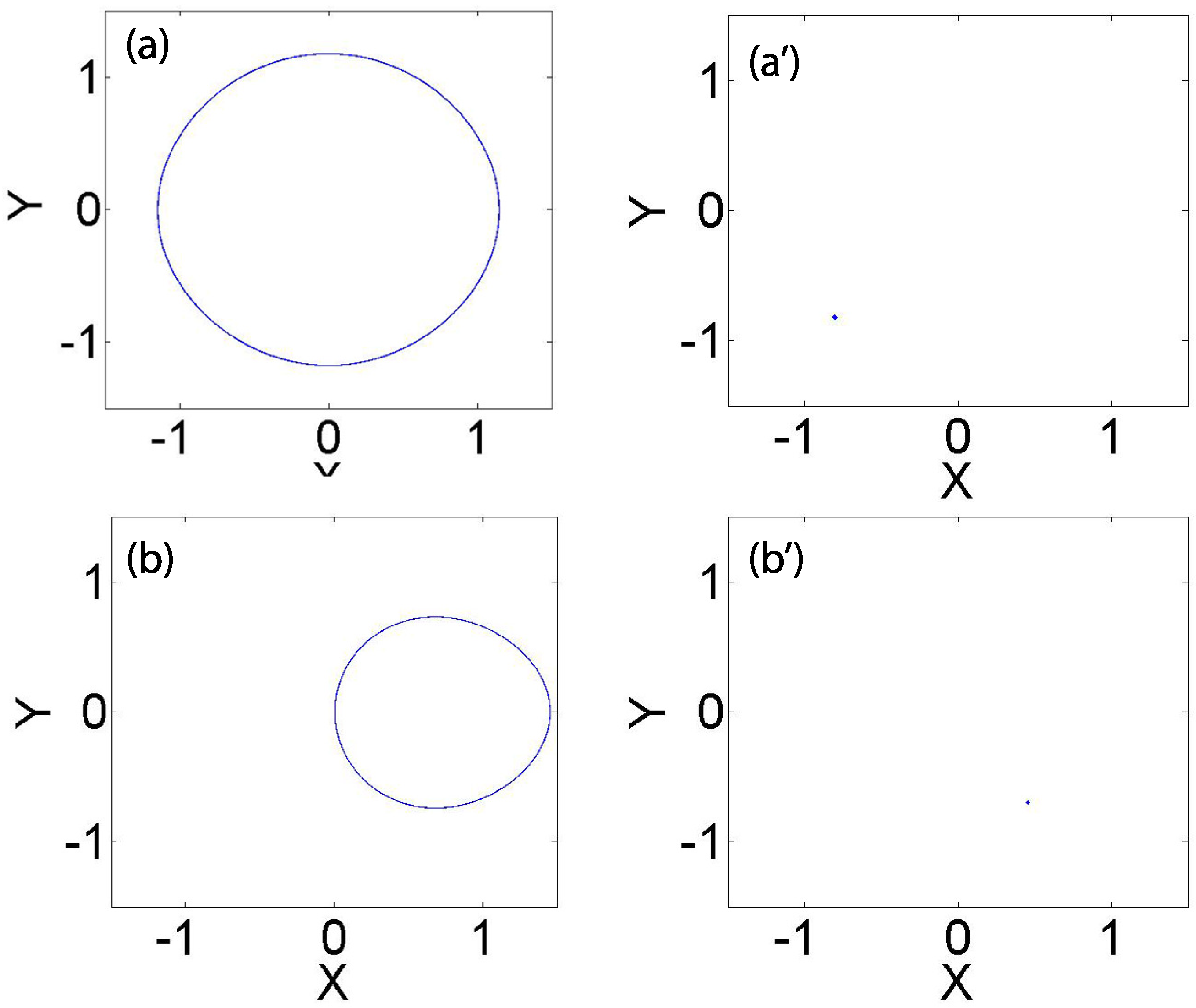
Our stroboscopic map corresponds to the Poincaré map with periodic excitation. This can be defined as the intersection of a periodic orbit in the space of a continuous dynamical system with a certain lower-dimensional subspace, called the Poincaré section, transversal to the flow of the system. A Poincaré map can be interpreted as a discrete dynamical system with a state space that is one dimension smaller than the original continuous dynamical system. This map qualitatively shows if the system is chaotic or not depending on the state points distribution. To define a stroboscopic map, we can consider a periodic orbit, with initial conditions within a section of the physical space. The periodic orbit leaves that section afterwards and we record the point at which it returns after one period. We repeat this procedure n times where $n\to \infty$ and therefore we complete the stroboscopic map. If the whole intersection is a set of r discrete points, where r is an integer and less than n, the trajectory is periodic of period equal to r. Otherwise, the trajectory is chaotic. A stroboscopic map is indeed a special case of a Poincaré map for periodic systems as in the case of pendulum oscillations. The distinguishing feature is that a given phase of the driver period is used for mapping (instead of some other marker event like a local maximum or a zero crossing). In our case, as the driving term is a $sin\left(\omega t\right)$ term, we build the stroboscopic map by mapping the state of the system in intervals of $2\pi$ time units.

Figure 2a,b,a’,b’ represent the numerical trajectories and the stroboscopic maps of the periodically driven pendulum with a torque. We observed different dynamical behaviors depending on the parameter values showing in phase portrait size and x mirror symmetry. We fixed the parameter values as $\alpha =0.15$, $f=0.25$, $\omega =1$ for both cases, while $\nu =0$ in Figure 2a,a’ and $\nu =0.55$ in Figure 2b,b’. Figure 2b,b’ clearly notes the external torque influence where periodic motions are present.

2.2. Vertically Excited Parametric Pendulum with a Torque

In the next case, we present the vertically excited parametric pendulum with a torque that has a suspension point subjected to a vertical periodic kinematic excitation. This kind of pendulum is also a classical example of chaotic system induced by the motion of the suspension point [9,23]; therefore, its dynamics is very rich and complex.

Figure 3 is given by the equation of motion [24]:

$$\begin{array}{ccc}\hfill & & m{l}^2\ddot{\varphi }+k\dot{\varphi }+m(gl-l\ddot{x})sin\varphi =N,\hfill \end{array}$$

(3)

where m and l denote the mass of the bob and the length of the pendulum, k is the damping coefficient, g is the gravity constant, and N is the extra constant torque. Additionally, $x\left(t\right)=asin\omega t$ represents the vertical periodic forcing of the suspension point of amplitude a and frequency $\omega$. The dimensionless form of this equation obtained dividing both sides of Equation (3) by $m{l}^2$, is the following:

$$\begin{array}{ccc}\hfill & & \ddot{\varphi }+\alpha \dot{\varphi }+(1+\gamma {\omega }^{2}sin\omega t)sin\varphi =\nu ,\hfill \end{array}$$

(4)

where ${\omega }_0=\sqrt{g/l}$ and as in the first model, its value is taken as ${\omega }_0=1$, $\alpha =k/\left(m{l}^2\right)$, $\gamma =a/l$ and $\nu =N/\left(m{l}^2\right)$.

In the case of the absence of the excitation terms (in Equations (2) and (4)) the shape of the potential can be expressed as:

$$\begin{array}{c}\hfill V\left(\varphi \right)=1-cos\varphi +\nu \varphi .\end{array}$$

(5)

This potential function is plotted in Figure 4 for different values of the torque $\nu =0.0,0.2,$ and $0.4$. Term $\nu$ breaks mirror symmetry $V\left(\varphi \right)=V(-\varphi )$.

Figure 5a,b,a’,b’ represent the numerical trajectories and the stroboscopic map of the vertically excited parametric pendulum with a torque. Again, on the basis of corresponding phase portraits, we observed some differences in dynamical responses depending on the parameter values. However, the Poincaré maps are represented by singular points informing about the agreement between system input and output periodicity (similarly as in Figure 2). We fixed the parameter values as $\alpha =0.15$, $\gamma =1$, $\omega =1$ for all cases, while $\nu =0$ in Figure 5a,a’, and $\nu =0.6$ in Figure 5b,b’.

Both pendula are often used as paradigmatic models of chaotic systems. This means that a tiny change in the initial parameters can cause huge changes in the dynamics of the system after a short period of time, as we show later. Then, after introducing the models of the pendula, we start the study of the excited pendulum with a torque in the limit of fast vertical kinematic oscillations to show how this kind of oscillations can affect the dynamics of the system and the potential shape.

3. Vibration of the Parametrically Excited Pendulum with a Torque in the Limit of Very Fast Excitation

Here, we examine the limit of fast kinematic vertical excitations of the vertically excited parametric pendulum with a torque (Equation (4)). Namely, the small amplitude $\gamma \ll 1$ and large frequency $\omega /{\omega }_0\gg 1$ enable to perform the system averaging. Using the method of direct separation of motions [25], we introduce slow $z\left(\tau \right)$ and fast coordinates $\psi (\tau ,{\tau }_1)$, where $\tau =\omega t$ is the dimensionless time that we use in order to simplify the equations:

$$\begin{array}{ccc}\hfill & & \varphi \left({\tau }_0\right)=z\left({\tau }_0\right)+\left(\frac{1}{\omega }\right)\psi ({\tau }_0,{\tau }_1),\hfill \end{array}$$

(6)

where a slow time ${\tau }_0=\tau$, while ${\tau }_1$ is a fast time ${\tau }_1=\left(1/\omega \right)\tau$ and the time derivatives are defined respectively

$$\begin{array}{c}\hfill \frac{dx}{d\tau }=\frac{\partial x}{\partial {\tau }_0}\frac{d{\tau }_0}{\partial \tau }+\frac{\partial x}{\partial {\tau }_1}\frac{d{\tau }_1}{\partial \tau }=\frac{\partial x}{\partial {\tau }_0}+\frac{1}{\omega }\frac{\partial x}{\partial {\tau }_1}=\dot{x}+\frac{1}{\omega }{x}^{\prime },\end{array}$$

(7)

where $\partial x/\partial {\tau }_0\equiv \dot{x}$ and $\partial x/\partial {\tau }_1\equiv x^{\prime }$. Additionally, the fast coordinate should fulfil the vanishing average condition:

$$\begin{array}{c}\hfill \overline{\psi }\left(\tau \right)=\frac{1}{2\pi }{\int }_0^{2\pi }\psi (\tau ,{\tau }_1)\mathrm{d}\tau =0\end{array}$$

(8)

By substituting Equations (6)–(8) into Equation (4) with the Taylor expansion of $sin(z+\frac{1}{\omega }\psi )$ and some algebra, we obtain:

$$\begin{array}{c}\hfill {\psi }^{″}=\gamma \omega sin{\tau }_1-\left(\frac{1}{\omega }\right)(\ddot{z}+2{\dot{\psi }}^{\prime }+\alpha (\dot{z}+{\psi }^{\prime })+sinz-\gamma \omega \psi coszsinz-\nu )+O\left(\omega \right).\end{array}$$

(9)

After averaging (and using Equation (8)), the final equation of motion for a slow motion can be expressed as (see [25], where $\nu =0$):

$$\begin{array}{c}\hfill \ddot{z}+\alpha \dot{z}+\left(1+\frac{1}{2}{\left(\gamma \omega \right)}^{2}cosz\right)sinz=0,\end{array}$$

(10)

producing new equilibria at $z=\pm \pi$ corresponding to an inverted pendulum.

In our more general case, the effective potential $V_{eff}\left(z\right)$ in the limit of very high frequency $\omega$ can be written as:

$$\begin{array}{c}\hfill V_{eff}\left(z\right)=1-cosz-\frac{{\left(\gamma \omega \right)}^2}{8}cos2z-\nu z,\end{array}$$

(11)

which is plotted in Figure 6b.

4. Melnikov Analysis

Here, we continue the study of our physical systems by applying Melnikov analysis in order to find the threshold parameter values for which the systems possess homoclinic chaos. The first step to begin with Melnikov analysis is to assume that damping parameter $\alpha$ and excitation amplitudes f (in the periodically driven pendulum with a torque) and $\gamma$ (in the vertically excited parametric pendulum with a torque) are fairly small, and a first-order perturbation could be used. By introducing a small parameter $ϵ$, we produce the substitutions $\alpha =ϵ\tilde{\alpha }$ and $\gamma =ϵ\tilde{\gamma }$, and we can rewrite the equations of motion (Equations (2) and (4)) as the two differential equations that we can find in

Table 1. The equations of the two pendulum models rewritten after the introduction of small parameter $ϵ$. The tilde is neglected in further notation.

Periodically Driven Pendulum with a Torque	Vertically Excited Parametric Pendulum with a Torque
$\dot{\varphi }=v_{\varphi }$	$\dot{\varphi }=v_{\varphi }$
${\dot{v}}_{\varphi }=-ϵ\alpha \dot{\varphi }-sin\varphi +\nu +ϵfsin\omega \tau$	${\dot{v}}_{\varphi }=-ϵ\alpha \dot{\varphi }-(1+ϵ\gamma {\omega }^{2}sin\omega \tau )sin\varphi +\nu$

, in which $v_{\varphi }$ is the angular velocity.

The corresponding Hamiltonian of the unperturbed system ($ϵ=0$) is

$$\begin{array}{ccc}\hfill & & H_0\left(\varphi \right)=\frac{v_{\varphi }^2}{2}+V\left(\varphi \right),\hfill \end{array}$$

(12)

where $V\left(\varphi \right)=1-cos\varphi +\nu \varphi$ is the unperturbed potential plotted in Figure 4. For $\nu =0$, $V\left(\varphi \right)$ corresponds to the potential of the pendulum. In that case, we can find the heteroclinic orbit connecting the saddle fixed points $\varphi =\pm \pi$ as shown in Figure 7. In order to evaluate the variation in the period, we obtain the reciprocal of Equation (12) and write $v_{\varphi }=\sqrt{2V\left(\varphi \right)}$ in the function of the unperturbed potential. Thus, the equation reads

$$\begin{array}{ccc}& & \frac{\mathrm{d}\tau }{\mathrm{d}\varphi }=\frac{1}{v_{\varphi }}=\frac{1}{\sqrt{2V\left(\varphi \right)}}\hfill \end{array}$$

(13)

and its integral is

$$\begin{array}{c}\hfill \tau -{\tau }_0=\int \frac{\mathrm{d}\varphi }{\sqrt{2-2cos\varphi }},\end{array}$$

(14)

where ${\tau }_0$ absorbs the integration constant.

It is possible to integrate the above expression, and after some algebra, we obtain the heteroclinic orbits

$$\begin{array}{ccc}& & {\varphi }^{*}=\pm 2arctan(sinh\tau )\hfill \\ & & v_{\varphi }^{*}=\pm \frac{2}{cosh(\tau -{\tau }_0)}.\hfill \end{array}$$

(15)

In Figure 8, we integrate numerically the equation

$$\begin{array}{c}\hfill \tau -{\tau }_0=\int \frac{\mathrm{d}\varphi }{\sqrt{2-2cos\varphi +2\nu \varphi }}.\end{array}$$

(16)

This expression corresponds to the case of the asymmetric potential with a nonzero torque, $\nu \ne 0$.

After adding perturbations, there is a split of the stable and the unstable manifolds, denoted by $W_S$ and $W_U$, so that they might intersect themselves creating a homoclinic point and generating the appearance of Smale’s horseshoe chaos. The distance $d\left(\tau \right)$ between the stable and unstable manifolds of the perturbed system is calculated along a direction that is perpendicular to the unperturbed homoclinic orbit. Then, the critical value for which the transition from periodic motions to chaos appears is found by setting the distance $d\left(\tau \right)$ to zero. This distance is related to the first order to the Melnikov function $M\left(\tau \right)$ in the following manner $d\left(\tau \right)=\epsilon \left(M\right(\tau )+O(\epsilon \left)\right)$, where $M\left(\tau \right)$ is given by:

$$\begin{array}{c}\hfill M\left(\tau \right)={\int }_{-\infty }^{\infty }{h}_0({\varphi }^{*},v_{\varphi }^{*})\wedge h_1({\varphi }^{*},v_{\varphi }^{*})\mathrm{d}\tau ,\end{array}$$

(17)

where ∧ defines the wedge product ($\mathrm{d}\varphi \wedge \mathrm{d}{v}_{\varphi }=-\mathrm{d}{v}_{\varphi }\wedge \mathrm{d}\varphi$, $\mathrm{d}\varphi \wedge \mathrm{d}\varphi =\mathrm{d}{v}_{\varphi }\wedge \mathrm{d}{v}_{\varphi }=0$), $h_0$ is the gradient of the unperturbed Hamiltonian

$$\begin{array}{ccc}& & h_0=(-sin{\varphi }^{*}+\nu )\mathrm{d}\varphi +v_{\varphi }^{*}\mathrm{d}v,\hfill \end{array}$$

(18)

and $h_1$ is a perturbation form to the same Hamiltonian which can be written as

$$\begin{array}{ccc}& & h_1=(-\alpha v_{\varphi }^{*}-\gamma {\omega }^{2}sin\omega \tau )sin{\varphi }^{*}\mathrm{d}\varphi .\hfill \end{array}$$

(19)

It is important that $h_0$ and $h_1$ are defined on the homoclinic orbits $(\varphi ,v_{\varphi })=({\varphi }^{*},v_{\varphi }^{*})$.

Thus, Melnikov function $M\left(\tau \right)$ reads:

$$\begin{array}{ccc}& & M\left(\tau \right)={\int }_{-\infty }^{\infty }{v}_{\varphi }^{*}(\tau -{\tau }_0)(\alpha v_{\varphi }^{*}(\tau -{\tau }_0)-\gamma {\omega }^{2}sin\omega \tau )sin{\varphi }^{*}(\tau -{\tau }_0)\mathrm{d}\tau .\hfill \end{array}$$

(20)

The condition for the intersection between the stable and unstable manifolds to happen is clearly $d\left(\tau \right)=0$, what implies that $M\left(\tau \right)=0$. Hence, we can write that the condition for the global homoclinic transition can be written as:

$$\begin{array}{c}\hfill \underset{\tau }{\bigvee }M\left(\tau \right)=0\mathrm{and}\frac{\partial M\left(\tau \right)}{\partial \tau }\ne 0.\end{array}$$

(21)

Lastly, for $\nu =0$, the mathematical expression for the critical parameter is:

$$\begin{array}{ccc}& & {\eta }_c^{\prime }=f/\alpha =\frac{4}{\pi {\omega }^4}sinh\left(\frac{\omega \pi }{2}\right).\hfill \end{array}$$

(22)

$$\begin{array}{ccc}& & {\eta }_c^{\prime \prime }=\gamma /\alpha =\frac{4}{\pi {\omega }^4}sinh\left(\frac{\omega \pi }{2}\right).\hfill \end{array}$$

(23)

We represent the corresponding Melnikov critical curves in Figure 9. In particular, Melnikov critical curves ${\eta }_c^{\prime }=f/\alpha$ versus frequency $\omega$ for the applied torques $\nu =0$, $0.02$, $0.04$, $0.06$ for the periodically driven pendulum with a torque, are represented in Figure 9a–d. On the other hand, Melnikov critical curves ${\eta }_c^{″}=\gamma /\alpha$ versus frequency $\omega$, for $\nu =0$, $0.2$, $0.4$, $0.6$, for the vertically excited parametric pendulum with a torque are plotted in Figure 9e–h. For values of the parameters above the critical values represented in the curve, the motion are chaotic, while become periodic otherwise. Interestingly, the curves that are shown in Figure 9c,f–h, for $\nu \ne 0$, could be caused by the more important influence of longer homoclinic orbits comparing to the heteroclinic orbits. In fact, the asymmetric potential makes the phenomenon of the resonance due to external perturbations are more probable. Therefore, the motion of the system could suffer a direct transition to a rotation regime, instead of showing chaotic solutions. The curves are reliable in the limit of small forcing and damping parameters.

5. Evolution of the Basins of Attraction

The basins of attraction provide relevant information on both the topology and the dynamics of the pendula. A basin of attraction [1] is the set of initial conditions that leads to a certain attractor of the system. When two or more attractors are present in the same region of phase space, obviously we need to use different colors, each one for each basin. Here, each basin is related with either a different mode of oscillation or rotation. The blue and pink basins correspond to oscillations for lower values of the torque $\nu$. The darker blue basins correspond to rotations for higher values of the torque $\nu$. We plot the basins of attraction using the software DYNAMICS [26] for the pendula by setting the parameter accordingly to the results of Figure 9. Figure 10a–d show the basins of attraction for the fixed values of the parameter, $\alpha =0.15$ and $\omega ={\omega }_0=1$ and different values of the parameters f and $\nu$. It is possible to see that the choice of these two last parameters is crucial for the dynamics of the system. In particular, in Figure 10c, for $f=2.5$ and $\nu =0$, the typical chaotic attractor, denoted by the green dots, shows up in the phase space and corresponds with chaotic motions, as predicted in Figure 9a–d. Then, in order to better understand the different behaviors shown in the previous section, we are going to analyze the evolution of the basins of attraction of the vertically excited parametric pendulum system with a torque for different values of the parameters $\nu$ and $\gamma$ in two different situations, $\omega =2$ (Figure 11) and $\omega =3$ (Figure 12), again varying the parameters according to the results shown in Figure 9e–h. In Figure 11 and Figure 12 the effect of the torque is relevant in the sense that the new basins appear insofar we vary $\nu$.

6. Conclusions

To summarize, we analyzed the nonlinear response of two planar pendula under a constant torque and various variable excitations. For better insight into their dynamics, we used typical approaches to nonlinear systems, such as the stroboscopic map, the Melnikov method, and the basins of attraction. For the Melnikov application, we used the semianalytical approach. Namely, we used the analytic forms of the Melnikov function, and the numerical homoclinic and heteroclinic orbits to improve the computational accuracy of critical conditions. Additionally, the vibration of pendula with a torque was studied in the limit of very fast excitation. Our results are the essential supplement to the available published materials and textbooks on the pendulum [27,28,29,30,31,32,33].

We proved that all these results faithfully correspond with the numerical simulations. In particular, escapes from the potential wells are accompanied by destructions of basins attractions corresponding to different multiple solutions.

Furthermore, using the dedicated nonlinear tools, we report characteristics of the complex dynamics that cannot be obtained from the direct integration of the equations of motions. In the next step, we would study the extended systems with the influence of magnetic field interactions and different models of friction.