Acoustic Propagation Characteristics of Unsaturated Porous Media Containing CO₂ and Oil

Abstract

Carbon dioxide geological utilization and storage (CGUS) is an effective way to mitigate climate warming. In this paper, we resorted to Lo’s model to analyze the dispersion and attenuation characteristics of unsaturated porous media. Based on this, we analyzed the sensitivity of the first compressional wave (P1) and the shear wave (S) to various physical parameters. In addition, the modified models of live oil’s velocity and density were proposed, which were verified by experimental data under the consideration of CO₂ dissolution. It is shown that the velocities and attenuations of P1 and S waves are influenced by various parameters, especially CO₂ saturation and pore fluid parameters, such as density and velocity. In particular, with increasing CO₂ saturation, the sensitivity of P1 velocity decreases, while that of the S velocity increases. Better monitoring results can be achieved by combining P1 and S waves. Finally, the acoustic response was analyzed under the modified model. With the increase in CO₂ saturation, the P1 velocity decreases, while the S velocity becomes almost constant and then linearly increases, with the trend changing at the critical saturation. The study provides a more precise basis for monitoring the security of CO₂ injection in CGUS.

1. Introduction

With the intensification of the greenhouse effect, carbon capture and storage (CCS) and carbon capture, utilization, and storage (CCUS) have attracted much attention in recent years [1]. Carbon dioxide (CO₂) geological utilization and storage (CGUS) is one of the most common methods to achieve CCUS. However, it requires careful monitoring to ensure the security of CGUS [2]. Seismic monitoring is an essential technology with the advantages of a wide detection range and high accuracy [3]. For seismic monitoring, it is vital to clarify the physical nature of acoustic wave propagation with varying environmental parameters, which can be used in identifying CO₂ migration status, spatial distribution, and providing guidance for CGUS strategy.

Most underground formations can be classified as porous media; the fluid-holding capacity of pore space is the basis for CGUS. When CO₂ is injected into the reservoir, the pore fluid is replaced by CO₂, accompanying the dissolution effect, which affects the energy exchange of the acoustic wave [4]. Thus, understanding the changes of seismic attributes form the foundations for successful monitoring. Therefore, analyzing the wave propagation in the reservoir filled with supercritical CO₂ and other fluids is crucial. In particular, changes in CO₂ injection in pore fluid parameters via different temperatures and pressures significantly impact how waves propagate.

Formations in CGUS are typical unsaturated porous media, composed of a solid grain and two fluids (usually CO₂ and oil in the oil reservoir), where acoustics theories for multi-phase porous media are appropriate for studying wave propagations [5]. To date, many models have described the porous media saturated by two immiscible fluids, such as Biot–Gassmann–Wood (BGW) theory [6,7,8], White’s model [9], Johnson’s model [10], the Biot–Rayleigh (BR) theory [11], Santos’s model [12] and Lo’s model [13,14]. Among them, the BGW theory is based on the effective media theory, which can be used at low frequencies [15]. The BR, White, and Johnson’s models describe patchy saturation’s mesoscopic dissipation mechanisms [16]. Santos and Lo’s models are the theory of the unsaturated porous media, considering both changes in capillary pressure and inertial and viscous coupling. Santos’s model is derived on the Lagrangian description, and Lo’s model is deduced on the Eulerian description. Compared with Santos’s model, Lo’s model derives from basic equations of the dynamic problem and the equation of state, and provides a detailed mathematical description of viscous coupling parameters, so that the parameters have clearer physical meaning. Currently, the BGW theory is commonly used in the seismic monitoring of CGUS [17]. However, the essence of this model is still a fluid–solid porous media, which replaces the parameters in Biot theory with the equivalent parameters of the mixed fluid. As a result, the BGW theory ignores fluid–fluid interactions [18]. In contrast, Lo’s model considers the coupling of fluid–fluid, which is more suitable to match the actual situation of unsaturated porous media in CGUS. Lo [13,14] validated the correctness by degenerating the model into the fully saturated porous media (Biot [6,7]; Berryman [19]) and the unsaturated porous media (Santos [12]; Tuncay [20]). Jardani [21] used Lo’s model to analyze the acoustic propagation in the unsaturated porous media.

The fluid type, CO₂ content, and dissolution are the key factors causing changes in pore fluid parameters [22]. In the monitoring of CGUS, many scholars used Batzle’s model [23] to describe the gas dissolution effect on fluid parameters [17]. Batzle’s model was proposed for hydrocarbon gases. The influence of hydrocarbon gases and CO₂ on oil, however, are different [24]. Therefore, it is inaccurate to treat CO₂ as a hydrocarbon gas. Han developed a preliminary model to explain the velocity and density of live oil (Han’s model) [24], but the model has limits when used with other oil samples.

The above studies show that it is necessary to understand the acoustic propagation of unsaturated porous media for seismic monitoring. The current models, however, cannot consider the influence of fluid–fluid interactions and is not accurate enough to describe the physical parameters of the CO₂–oil mixtures. Therefore, to precisely illuminate the acoustic properties of porous media during CO₂ injection, a more realistic model, including the pore fluid parameter models and the unsaturated porous media model should be used.

In this paper, we selected Lo’s model to describe the acoustic propagation in unsaturated porous media, considering the dissolution effect of CO₂. With the change of frequency and CO₂ saturation, we calculated the phase velocities and attenuations of four mode waves (three types of compressional waves and one shear wave). We analyzed the sensitivity of phase velocities and attenuations of P1 and S, which reflected the importance of pore fluid parameters for monitoring. Furthermore, we modified the live oil’s density and velocity models and validated them against experimental data. Finally, we compared the application of the fluid parameter models before and after the correction.

2. Fundamental Theory

Considering the influences of inertial coupling and viscous coupling, the motion equation of unsaturated porous media can be obtained, which is aided by the closure relation for porosity change and the balance of mass and momentum. For a more concise representation, the equation of motion is expressed as the vector–matrix form (Equation (1)). The description of the 3D three-component form of the motion equation is given in Appendix B.

$$\mathsf{\rho }\ddot{u}+A\ddot{u}+R\dot{u}=M\nabla \nabla \cdot u+N\nabla \cdot \nabla u,$$

(1)

where $u={\left[{\overrightarrow{u}}^s,{\overrightarrow{u}}^1,{\overrightarrow{u}}^2\right]}^T$ denotes the displacement matrix; the superscripts s, 1, and 2 refer to the solid grain, the nonwetting fluid, and the wetting fluid, respectively; $\mathsf{\rho }$ denotes the mass densities matrix; A denotes the inertial coefficients matrix; R denotes the viscous coefficients matrix; M denotes the rigidity moduli matrix; and N denotes the shear moduli matrix. $\mathsf{\rho }$, A, R, M, and N are given by [14]:

$$\begin{array}{l}\mathsf{\rho }=\left[\begin{array}{ccc}{\rho }_s\left(1-\varphi \right)& 0& 0\\ 0& {\rho }_1{S}_1\varphi & 0\\ 0& 0& {\rho }_2{S}_2\varphi \end{array}\right],M=\left[\begin{array}{ccc}{a}_{11}+N/3& a_{12}& a_{13}\\ a_{12}& a_{22}& a_{23}\\ a_{13}& a_{23}& a_{33}\end{array}\right],N=\left[\begin{array}{ccc}N& 0& 0\\ 0& 0& 0\\ 0& 0& 0\end{array}\right],\\ A=\left[\begin{array}{ccc}-A_{11}-2A_{12}-A_{22}& A_{11}+A_{12}& A_{12}+A_{22}\\ A_{11}+A_{12}& -A_{11}& -A_{12}\\ A_{12}+A_{22}& -A_{12}& -A_{22}\end{array}\right],\\ R=\left[\begin{array}{ccc}-R_{11}-R_{22}-R_{12}-R_{21}& R_{11}+R_{21}& R_{12}+R_{22}\\ R_{11}+R_{12}& -R_{11}& -R_{12}\\ R_{21}+R_{22}& -R_{21}& -R_{22}\end{array}\right],\end{array}$$

(2)

where ${\rho }_l$ denotes the density of phase l, l = s, 1, 2; $\varphi$ is the porosity; S₁ is the saturation of nonwetting fluid, S₂ is the saturation of wetting fluid, and S₂ = 1 − S₁; N is the shear modulus; A₁₁ denotes the inertial coupling between solid grain and nonwetting fluid, A₂₂ denotes the inertial coupling between solid grain and wetting fluid, and A₁₂ is the inertial coupling between nonwetting fluid and wetting fluid; R₁₁ represents the viscous coupling between solid grain and nonwetting fluid, R₂₂ denotes the viscous coupling between solid grain and wetting fluid, R₁₂ and R₂₁ are the viscous coupling between nonwetting fluid and wetting fluid; a_ij (i, j = 1, 2, 3) denotes the elastic coefficients, which are derived from the closure relation for porosity change, the balance of mass, and the equation of state, as shown in Appendix A. We list A_ij, R_ij, and a_ij in Appendix A, which are functions of rock parameters ($\varphi$, $\kappa$, K_s, N, K_m, ${\rho }_s$) and fluid parameters (K₁, K₂, ${\rho }_1$, ${\rho }_2$, S₁, S₂).

According to the Helmholtz theorem, applying the divergence and rotational operators to the motion equation (Equation (1)), we can obtain the governing equations of compressional and shear waves:

$$\begin{array}{l}\mathsf{\rho }\ddot{\mathsf{\phi }}+A\ddot{\mathsf{\phi }}+R\dot{\mathsf{\phi }}=\left(M+N\right){\nabla }^2\mathsf{\phi },\\ \mathsf{\rho }\ddot{\mathsf{\psi }}+A\ddot{\mathsf{\psi }}+R\dot{\mathsf{\psi }}=N{\nabla }^2\mathsf{\psi }.\end{array}$$

(3)

where $\mathsf{\phi }={\left[{\phi }^s,{\phi }^1,{\phi }^2\right]}^T$, ${\phi }^l=\nabla ·{\overrightarrow{u}}^l$ represents the potential functions of compressional waves, l = s, 1, 2; $\mathsf{\psi }={\left[{\overrightarrow{\psi }}^s,{\overrightarrow{\psi }}^1,{\overrightarrow{\psi }}^2\right]}^T$, ${\overrightarrow{\psi }}^l=\nabla \times {\overrightarrow{u}}^l$ represents the potential functions of shear waves, l = s, 1, 2. The definition of potential functions in porous media also refers to Refs. [7,12,25].

Next, the governing equations (Equation (3)) are subjected to the steady-state analysis, i.e., the single-frequency plane waves (Equation (4)) are substituted into the governing equations (Equation (3)). The final governing equations of compressional and shear waves can be written as Equation (5).

$$\left(\begin{array}{c}{\phi }^s\\ {\phi }^1\\ {\phi }^2\end{array}\right)=\left(\begin{array}{c}{\alpha }^s\\ {\alpha }^1\\ {\alpha }^2\end{array}\right)\exp \left[i\left(k_p·r-\omega t\right)\right],\left(\begin{array}{c}{\overrightarrow{\psi }}^s\\ {\overrightarrow{\psi }}^1\\ {\overrightarrow{\psi }}^2\end{array}\right)=\left(\begin{array}{c}{\overrightarrow{\beta }}^s\\ {\overrightarrow{\beta }}^1\\ {\overrightarrow{\beta }}^2\end{array}\right)\exp \left[i\left(k_s·r-\omega t\right)\right],$$

(4)

where ${\alpha }^l$ and ${\overrightarrow{\beta }}^l$ are wave amplitudes; $\omega$ is the angular frequency; $k_p$ and $k_s$ are the complex wave number vectors of the compressional and shear waves, respectively.

$$\begin{array}{l}\left[-{\omega }^2\left(\mathsf{\rho }+A\right)-i\omega R+k_p{}^2\left(M+N\right)\right]\left(\begin{array}{c}{\alpha }^s\\ {\alpha }^1\\ {\alpha }^2\end{array}\right)=0,\\ \left[-{\omega }^2\left(\mathsf{\rho }+A\right)-i\omega R+k_s{}^2\left(N\right)\right]\left(\begin{array}{c}{\overrightarrow{\beta }}^s\\ {\overrightarrow{\beta }}^1\\ {\overrightarrow{\beta }}^2\end{array}\right)=0\end{array}$$

(5)

Therefore, we can obtain the dispersion relation of compressional (Equation (6)) and shear waves (Equation (7)).

$$\det \left(-{\omega }^2\left(\mathsf{\rho }+A\right)-i\omega R+k_p{}^2\left(M+N\right)\right)=0$$

(6)

$$\det \left(-{\omega }^2\left(\mathsf{\rho }+A\right)-i\omega R+k_s{}^2\left(N\right)\right)=0$$

(7)

Since the dispersion equation of compressional wave (Equation (6)) is a cubic polynomial in ${\omega }^2$/k_p², there exist six complex roots of k_p. With the physical constraint that the elastic wave always diminishes along the propagation direction (i.e., Im (k_p) > 0), we finally obtained three complex roots of Equation (6) about k_p. Similarly, we obtained one complex root about k_s in the dispersion equation of shear wave (Equation (7)). We used phase velocity v and inverse quality factor Q⁻¹ to analyze the dispersion and attenuation, which can be written as

$$\begin{array}{l}{v}_i=\omega /\mathrm{Re}\left(k_i\right), i=\mathrm{P}1, \mathrm{P}2, \mathrm{P}3, \mathrm{S},\\ Q_i{}^{-1}=2\mathrm{Im}\left(k_i\right)/\mathrm{Re}\left(k_i\right), i=\mathrm{P}1, \mathrm{P}2, \mathrm{P}3, \mathrm{S},\end{array}$$

(8)

where k_i denotes the roots of dispersion equations of compressional (Equation (6)) and shear waves (Equation (7)).

In summary, there are three types of compressional waves (the first compressional wave (P1), the second compressional wave (P2), and the third compressional wave (P3), respectively) and one shear wave (S) in unsaturated porous media. The phase velocities and attenuations of each mode wave are influenced by various factors, including rock parameters and fluid parameters. We will analyze the propagation characteristics of each mode wave via Lo’s model to explore the acoustic response of the unsaturated porous media during CGUS.

3. Numerical Analysis

3.1. Wave Modes Characteristics

According to the results in Section 2, we calculated the propagation characteristics of acoustic waves at different CO₂ saturations and frequencies, including phase velocities and attenuations in the porous media. The physical parameters of the porous media are presented in

Table 1. Physical parameters of unsaturated porous media.

Type	Parameters	Value
Utsira sand	grain bulk modulus, Ks (GPa)	40 1
	frame bulk modulus, Km (GPa)	1.37 1
	shear modulus, N (GPa)	0.82 1
	$\mathrm{grain} \mathrm{density}, {\rho }_s$ (kg/m3)	2600 1
	$\mathrm{porosity}, \varphi$	0.36 1
	$\mathrm{permeability}, \kappa$ (D)	1.6 1
Nonwetting fluid—CO2, (p = 10.3 MPa, T = 45 °C)	$\mathrm{density}, {\rho }_1$ (kg/m3)	539.07 2
	bulk modulus, K1 (MPa)	30.6 2
	$\mathrm{viscosity}, {\mu }_1$$(\mathsf{\mu }\mathrm{Pa}\cdot \mathrm{s}$)	38.9 2
	CO2 gravity, G	1.5281 2
Wetting fluid—oil, (p = 0.101 MPa, T = 25 °C)	$\mathrm{density}, {\rho }_0$ (kg/m3)	799 3
	$\mathrm{viscosity}, {\mu }_0$$(\mathrm{mPa}\cdot \mathrm{s}$)	2.76 3
	Molar Weight, MW (g/mol)	223 3

¹ The physical parameters of the solid grain are from Ref. [17]. ² The physical parameters of the nonwetting fluid are from Ref. [26]. ³ The physical parameters of the wetting fluid are from Ref. [27].

. In particular, we consider the dissolution effect on the live oil parameters, given by Batzle’s model [23].

We first examine the impact of CO₂ dissolution on the pore fluid’s phase state. Following Carcione’s work [17], we assume that when the CO₂ content in the pore is greater than the maximum CO₂ dissolution of crude oil, there are two phase fluids in the pore (live oil and free CO₂); otherwise, the pore contains one type of fluid (live oil). It can be written as [17]

$$S_1’=\{\begin{array}{l}0,S_1<S_c\\ \frac{S_1-S_c}{1-S_c},S_1\ge S_c\end{array},$$

(9)

where S₁′ denotes the actual CO₂ saturation after CO₂ dissolution; S₁ denotes the saturation of injection; S_c denotes the critical saturation, calculated by the maximum dissolution of crude oil, which can be written as

$$S_c=\frac{{\rho }_{CO2s}{\rho }_{oil}GOR}{{\rho }_{CO2}{\rho }_0+{\rho }_{CO2s}{\rho }_{oil}GOR},$$

(10)

where ${\rho }_{CO2s}$ and ${\rho }_{CO2}$ are the density of CO₂ at the surface (15.6 °C and 1 atm) and reservoir, respectively; ${\rho }_0$ and ${\rho }_{oil}$ are the density of crude oil at the surface and reservoir, respectively; GOR is the gas–oil ratio at the standard condition, which can be calculated by Emera [28].

According to the above description, we calculated the phase velocities and attenuations as functions of frequency and CO₂ saturation. The results are shown in Figure 1 and Figure 2. Firstly, the P1 and S waves propagate fairly fast and have low attenuation. Thus, the waves can be observed at the seismic exploration (10–100 Hz) frequency. In contrast, the P2 and P3 waves propagate slowly and have high attenuation, which is difficult to be observed at the seismic exploration frequency. Secondly, as frequency increases, the phase velocities of all four mode waves increase, and the attenuations of P2 and P3 decrease. That is because the effect of inter-fluid viscosity dominates in the low-frequency range. As the frequency increases, the inertial effect becomes increasingly dominant. Obviously, due to the dissolution effect, the phase velocities and attenuations of the four mode waves all change significantly at the critical saturation (42% in this case). When CO₂ saturation is less than critical saturation, the pore contains only one fluid. At this time, P3 has low velocity and high attenuation in the entire frequency range, without fluid–fluid interaction. When the critical saturation is exceeded, two fluids in the porous media interact with each other, resulting in a decrease in P2 velocity and an increase in P3 velocity. In addition, with the increase in CO₂ saturation, the transition zone between low and high frequencies of P3 moves toward high frequency, while P2 and S move toward low frequency.

From Figure 1 and Figure 2, we chose a typical seismic frequency (f = 100 Hz) to ensure each mode wave propagates more clearly. Figure 3 displays the results for the P1 wave and S wave. It can be observed in Figure 3 that when CO₂ saturation increases, the S velocity increases, while the P1 velocity decreases. At high CO₂ saturation, the change in P1 velocity is not obvious. This results from both the density and velocity of the pore fluid mixture. The pore fluid velocity significantly impacts the P1 velocity, which decreases as the fluid velocity decreases. Only the pore fluid density affects S velocity, which increases as the fluid density decreases. Due to the dissolution effect, the critical saturation marks the point at which the pore fluid changes from a single phase to two phases. When the free CO₂ appears, the attenuations of P1 and S increase rapidly. With the above results, we can expect that Lo’s model can be used for the seismic monitoring of CO₂ migration.

3.2. Sensitivity Analysis

Numerous factors influence the phase velocities and attenuations of the four mode waves, including CO₂ saturation, porosity, permeability, density, and velocity of pore fluid. The sensitivity can be used to describe the effect of each parameter on the phase velocities and attenuations at different frequencies. The sensitivity can be expressed as [29]

$$S_p\left(v\right)=\frac{p\partial v}{v\partial p},S_p\left(Q^{-1}\right)=\frac{p\partial Q^{-1}}{Q^{-1}\partial p},$$

(11)

where p denotes the media parameter; S_p denotes the sensitivity of p; and v and Q⁻¹ denote the velocity and inverse quality factor, respectively.

Sensitivity greater than or less than 0 indicates that the velocities and attenuations increase or decrease with increasing parameters. The sensitivities of different parameters to the velocities and attenuations of P1 and S are shown in Figure 4. Among them, the initial value of CO₂ saturation is taken as 0.5, and the initial values of other parameters are taken from Table 1.

The sensitivity of P1 and S velocities are independent of the frequency to all parameters in Figure 4. Among them, the increase in porosity increases the velocities of P1 and S, and the increase in CO₂ saturation decreases the velocity of P1 and increases the velocity of S. At the same time, permeability has almost no effect on the velocities of P1 and S. Moreover, the attenuations of P1 and S show the same pattern of sensitivity to pore fluid density, porosity, and permeability. Notably, the sensitivity of P1 and S attenuations to CO₂ saturation is higher than other parameters in Figure 4c,d, and the attenuation of P1 is more sensitive than that of S at seismic frequency. It indicates that using attenuation to monitor CO₂ migration is feasible. In addition, whereas the velocity of CO₂ and oil only affects the velocity and attenuation of P1 wave, the density has an impact on the velocities and attenuations of both P1 and S waves, which corresponds to the analysis in Figure 3. Obviously, the sensitivity of P1 to the pore fluid velocity is higher than that to the pore fluid density.

In CGUS, CO₂ saturation, the ultimate inversion result of seismic monitoring, is the underlying cause of the change in acoustic propagation characteristics. Therefore, we focus on the sensitivity of CO₂ saturation to the acoustic response, which represents the inversion accuracy of monitoring CO₂ migration. Figure 5 shows the sensitivity of P1 wave and S wave phase velocities to different CO₂ saturations, corresponding to the change in Figure 3. With CO₂ saturation increases, the sensitivity of the S velocity increases, while the sensitivity of P1 velocity initially increases and then decreases. Near the critical CO₂ saturation, the P1 velocity is most sensitive. It indicates that the closer to the critical saturation, the more precise the inversion of P1 velocity. Further, the inversion of P1 velocity is less reliable, and the inversion of S velocity is more reliable with higher CO₂ saturation. Therefore, the combined inversion of P1 and S can achieve better monitoring results.

For the porous media with certain porosity, the propagation characteristics of P1 and S are related to pore fluid parameters. Moreover, the density and velocity of the pore fluid are affected by various factors, such as temperature, pressure, and CO₂ saturation. It is an effective way to use the more precise fluid parameter model to reduce the uncertainty of seismic monitoring simulations.

4. Fluid Parameters Model Correction

4.1. Density Correction for the CO₂–Oil Mixture

Han developed an empirical model for the density of the gas–oil mixture [30], by introducing the effective density of the gas. On the basis of Han’s work, we proposed a density model for the CO₂–oil mixture, through the ideal mixing rule and the effective density of CO₂ (Saryazdi [31]). The model is expressed as follows:

$${\rho }_{o,\mathrm{CO}2}=\frac{{\rho }_0+W_{CO2}}{1+W_{CO2}/{\rho }_{a,\mathrm{CO}2}}+\Delta {\rho }_{P,T}+\Delta {\rho }_{X_{\mathrm{CO}2}},$$

(12)

where ${\rho }_{a,\mathrm{CO}2}$ denotes the effective density of CO₂; W_CO2 denotes the dissolved mass of CO₂; $\Delta {\rho }_{P,T}$ and $\Delta {\rho }_{X_{\mathrm{CO}2}}$ are temperature–pressure and solubility correction factors, respectively. The above parameters can be written as [30,31]

$$\begin{array}{ll}{\rho }_{a,\mathrm{CO}2}& =2.3349\exp \left[-0.003157\left(T+273.15\right)\right]·\exp \{4.12\times {10}^{-4}P+\\ & \left[-0.3233+0.001897\left(T+273.15\right)\right]\left[1-\exp \left(-1.37\times {10}^{-2}P\right)\right]\},\\ W_{CO2}& =0.001223*GOR*G,\\ \Delta {\rho }_{P,T}& =\Delta {\rho }_P-\Delta {\rho }_T+b_{00}+b_{01}T+b_{02}{T}^2+\left(b_{10}+b_{11}T\right)P,\\ \Delta {\rho }_{X_{\mathrm{CO}2}}& =b_{20}+b_{21}{X}_{\mathrm{CO}2},\end{array}$$

(13)

where P is the reservoir pressure; T is the reservoir temperature; $\Delta {\rho }_P$ and $\Delta {\rho }_T$ are given in Han [30]; $b_{ij}\left(i,j=0,1,2\right)$ is the fitting parameter, obtained from the experimental data in Calabrese [32] and given in

Table 2. Fitting correction coefficients of temperature–pressure and solubility correction factors in Equation (13).

bij	j = 0	j = 1	j = 2
i = 0	4.034 × 10−3	1.319 × 10−4	−5.814 × 10−7
i = 1	−7.016 × 10−5	−1.286 × 10−6
i = 2	−5.85 × 10−4	2.477 × 10−2

; X_CO2 denotes the mole fraction of CO₂ in crude oil.

Figure 6 depicts the measured values (Calabrese [32]) of density in the CO₂–oil mixture, compared with the density of Han’s model [24] and the modified model in this paper. The correlation coefficient of Han’s model is 0.7548, and the modified model is 0.9807. As shown in Figure 6, the predicted densities resulting from the modified model are generally consistent with the experimental data. The modified model achieved better application results.

To verify the applicability of the modified model, we compare the predicted densities with measured densities in different oil samples, as shown in Figure 7. Due to the differences in oil samples, environment, and other factors, the model prediction results may be slight deviations from the experimental data. In this case, we could fit a correction for b_ij by Table 2 and the experimental data. The solid lines in Figure 7 are the results of the corrected model. In summary, compared with the density model of Han’s model, the modified model for live oil’s density has a more efficient physical meaning and considers the effect of CO₂ solubility. The modified model can be obtained by simple coefficient correction for a certain oil sample, which has better applicability.

4.2. Velocity Correction for the CO₂–Oil Mixture

Han proposed a model for the velocity of the CO₂–oil mixture at various temperatures, pressures, and CO₂ solubilities, expressed as [24]

$$V=A-BT+C\left(\frac{1-D^P}{1-D}\right)+FTP,$$

(14)

where A, B, C, D, and F are functions of ${\rho }_{v\_seu}$, given in Han [24]. ${\rho }_{v\_seu}$ denotes the velocity pseudo density of live oil, written as [24]

$$\begin{array}{l}{\rho }_{a1}=M_{s1}+M_{s2}API+\left(N_{s1}+N_{s2}API\right)\ln \left(G\right),\\ {\rho }_{a2}=\left[M_g+N_g\left(\frac{1+W_{CO2}/{\rho }_0}{1+W_{CO2}/{\rho }_{a1}}\right)\right]{\rho }_{a1},\\ {\rho }_{v\_seu}=\frac{{\rho }_0+\epsilon W_{CO2}}{1+W_{CO2}/{\rho }_{a2}},\end{array}$$

(15)

where API denotes the oil gravity, developed by American Petroleum Institute (API); M_s1, M_s2, N_s1, N_s2, M_g, and N_g are experimental fitting parameters, which are related to the CO₂ gravity (G) and the dissolution effect. $\epsilon$ is the effective gas parameter, which indicates the contribution of the gas to the pseudo-liquid velocity, $\epsilon =0.113$ in this paper [24].

As can be seen in Figure 8a, Han’s model overestimates the velocities of the CO₂–oil mixture, which may result from the overestimation of the contribution of CO₂ solubility to pseudo density. We performed a parameter fitting correction for the parameters related to CO₂ solubility, including M_s1, M_s2, N_s1, N_s2, M_g, and N_g. In order to find the best correction parameters, a part of the experimental data (Ratnakar [35]) was selected for parameter fitting correction, and the others were used as the validation data of the corrected model. The correlation coefficient (R²) was used to evaluate the reliability of the model predictions, and the results are shown in

Table 3. Comparison of correlation coefficients (R²) of different correction parameters.

Range of Experimental Data (46 Data Points in Total)	R2 of Correction for (Mg, Ng)	R2 of Correction for (Ms1, Ms2)	R2 of Correction for (Ns1, Ns2)
P ≤ 40 MPa (22 data points)	0.9927	0.9634	0.9633
T ≤ 40 °C (23 data points)	0.9931	0.9629	0.9630
XCO2 ≥ 40% (15 data points)	0.9644	0.9637	0.9637
XCO2 ≥ 8% (31 data points)	0.9943	0.9637	0.9636
Random (20 data points)	0.9940	0.9636	0.9633
Random (10 data points)	0.9896	0.9637	0.9608

. The combination of M_g and N_g has the best correction effect, which can produce better predictions with fewer data. The fitted parameters of the modified model are M_g = 8.8680, N_g = −8.5132. The results of the corrected model are shown in Figure 8b.

In summary, this section proposes a modified method for the density and velocity models of the CO₂–oil mixture, respectively. The density-modified model can be referred to Equations (12) and (13), and the velocity-modified model can be referred to Equations (14) and (15). Due to differences in regions and oil samples, there may be deviations between the measured and predicted data. At this time, the parameters could be corrected according to the specific experimental data (b_ij for the density model; M_g and N_g for the velocity model).

5. Propagation Characteristics under the Modified Model

Following the previous section, we obtained the modified models for live oil’s density and velocity, which are the functions of temperatures, pressures, and CO₂ solubility. It provides a basis to accurately describe the changes of the pore fluid physical parameters in CGUS. Figure 9 shows the phase velocities and attenuations of P1 and S waves at different CO₂ saturation and frequencies, combining Lo’s model and the modified models of fluid parameters.

Comparing Figure 1, Figure 2 and Figure 9, it can be seen that the trend of wave velocities and attenuations with frequency and CO₂ saturation in Figure 9 is essentially unchanged, except for the S velocity. In fact, the velocity of S is almost constant before the critical saturation because of little change in the live oil’s density due to CO₂ dissolution. After the critical saturation, the velocity of S linearly increases with increasing free CO₂. To show the effect of fluid parameters models more obviously, we calculated the P1 and S phase velocities and attenuations at the typical seismic frequency (f = 100 Hz), as shown in Figure 10. The fluid parameters of Batzle’s model overestimate the attenuations of P1 and S. There is a considerable variation in the prediction of S velocity, with a lower prediction for P velocity at low CO₂ saturation and a higher prediction at high CO₂ saturation. The above results indicate that the fluid parameters of Batzle’s model are inaccurate for characterizing the physical parameters of the CO₂–oil mixture.

6. Conclusions

In this paper, we proposed Lo’s model to study the effect of CO₂ injection on the acoustic responses of the porous media containing two immiscible fluids. We calculated the variation of phase velocities and attenuations of waves, with frequency and CO₂ saturation. In addition, we analyzed the sensitivities of phase velocities and attenuations to various parameters, especially CO₂ saturation. Moreover, we proposed a method to modify the velocity and density models of the CO₂–oil mixture based on experimental data. Finally, the wave propagation was compared between Batzle’s model and the modified model under Lo’s model. The conclusions are as follows:

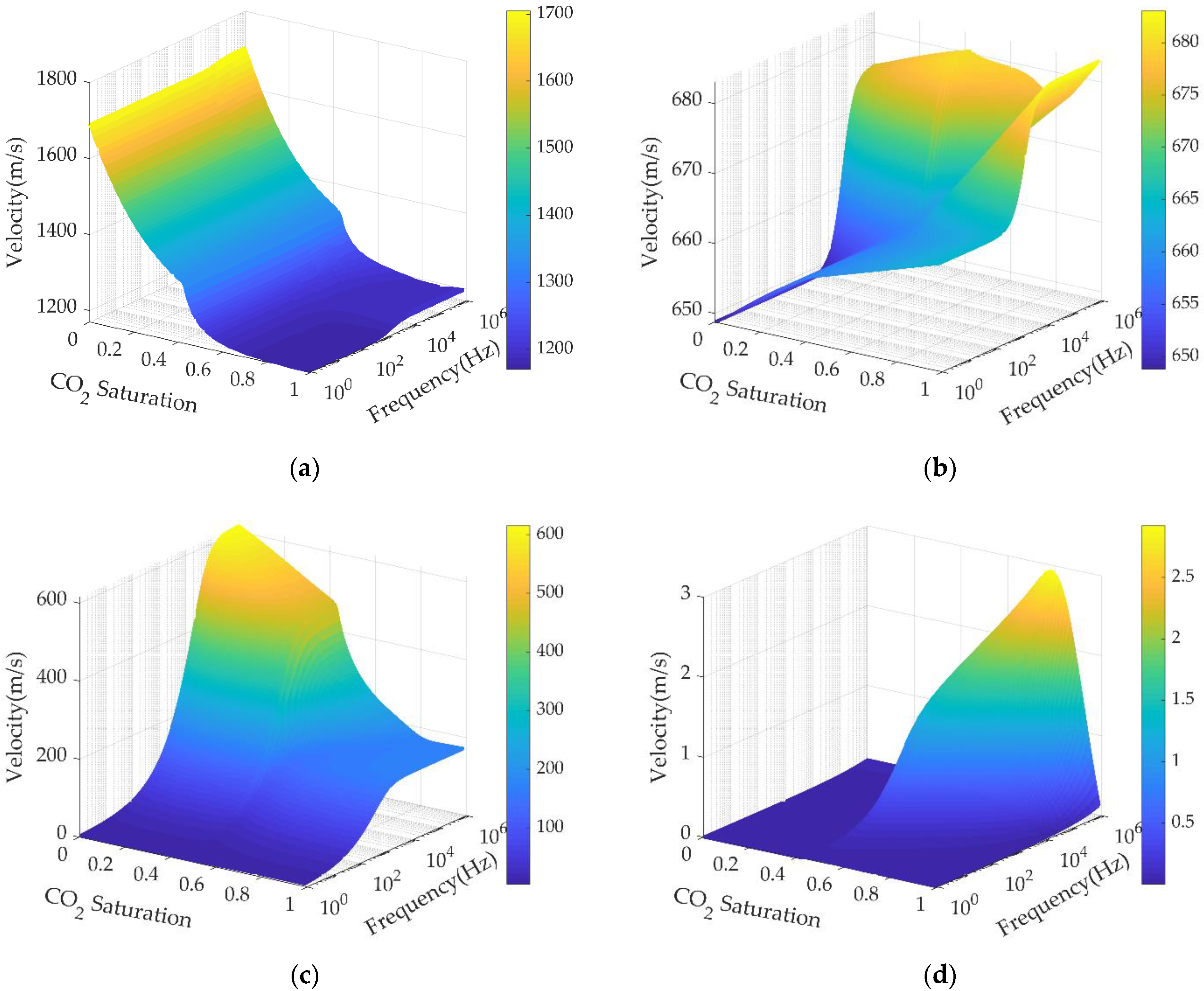
• There are four kinds of mode waves (three compressional waves and one shear wave) in the unsaturated porous media with pore fluid composed by CO₂ and oil. However, only two mode waves, P1 and S, can be observed at seismic frequencies. The velocity and attenuation characteristics are sensitive to CO₂ saturation, and the combined P1 and S waves can monitor the CO₂ migration more accurately.
• In the analysis of acoustic wave modes, the accuracy of the features of pore fluid is crucial. The pore fluid density has an effect on both the velocities and attenuations of P1 and S, while the pore fluid velocity only has an effect on the velocity and attenuation of P1.
• The fluid parameter of Batzle’s model is based on hydrocarbon gas, which cannot accurately describe the physical parameters of the CO₂–oil mixture. Compared with experimental data, the modified model can provide more exact data.

The numerical simulations show that Lo’s model, combined with the modified parameters models of live oil, can realistically describe the wave propagation characteristics of unsaturated porous media. The velocities and attenuations of waves in unsaturated porous media are closely related to CO₂ saturation, considering the effect of dissolution, temperature, and pressure. The model of pore fluid parameters and the theory of unsaturated porous media in this paper can be used to explore the changing pattern of the acoustic field after CO₂ injection. Meanwhile, this study provides a more accurate basis to monitor the security of CO₂ injection in CGUS.

References

1. Lee, H.S.; Cho, J.; Lee, Y.W.; Lee, K.S. Compositional Modeling of Impure CO2 Injection for Enhanced Oil Recovery and CO2 Storage. Appl. Sci. 2021, 11, 7907. [Google Scholar] [CrossRef]
2. Harbert, W.; Goodman, A.; Spaulding, R.; Haljasmaa, I.; Crandall, D.; Sanguinito, S.; Kutchko, B.; Tkach, M.; Fuchs, S.; Werth, C.J.; et al. CO2 induced changes in Mount Simon sandstone: Understanding links to post CO2 injection monitoring, seismicity, and reservoir integrity. Int. J. Greenh. Gas Control 2020, 100, 103109. [Google Scholar] [CrossRef]
3. Li, D.; Peng, S.; Guo, Y.; Lu, Y.; Cui, X. CO2 storage monitoring based on time-lapse seismic data via deep learning. Int. J. Greenh. Gas Control 2021, 108, 103336. [Google Scholar] [CrossRef]
4. Maurya, S.P.; Singh, N.P. Seismic modelling of CO2 fluid substitution in a sandstone reservoir: A case study from Alberta, Canada. J. Earth Syst. Sci. 2019, 128, 236. [Google Scholar] [CrossRef]
5. Liu, L.; Zhang, X.; Wang, X. Wave Propagation Characteristics in Gas Hydrate-Bearing Sediments and Estimation of Hydrate Saturation. Energies 2021, 14, 804. [Google Scholar] [CrossRef]
6. Biot, M.A. Mechanics of deformation and acoustic propagation in porous media. J. Appl. Phys. 1962, 33, 1482–1498. [Google Scholar] [CrossRef]
7. Biot, M.A. Generalized theory of acoustic propagation in porous dissipative media. J. Acoust. Soc. Am. 1962, 34, 1254–1264. [Google Scholar] [CrossRef]
8. Mavko, G.; Mukerji, T.; Dvorkin, J. The Rock Physics Handbook; Cambridge University Press: Cambridge, UK, 2009; pp. 175–177. ISBN 978-0-511-65062-8. [Google Scholar]
9. White, J.E. Computed seismic speeds and attenuation in rocks with partial gas saturation. Geophysics 1975, 40, 224–232. [Google Scholar] [CrossRef]
10. Johnson, D.L. Theory of frequency dependent acoustics in patchy-saturated porous media. J. Acoust. Soc. Am. 2001, 110, 682–694. [Google Scholar] [CrossRef]
11. Ba, J.; Carcione, J.M.; Cao, H.; Du, Q.Z.; Yuan, Z.Y.; Lu, M.H. Velocity dispersion and attenuation of P waves in partially-saturated rocks: Wave propagation equations in double-porosity medium. Chin. J. Geophys. 2012, 55, 219–231. [Google Scholar]
12. Santos, J.E.; Douglas Jr, J.; Corberó, J.; Lovera, O.M. A model for wave propagation in a porous medium saturated by a two-phase fluid. J. Acoust. Soc. Am. 1990, 87, 1439–1448. [Google Scholar] [CrossRef]
13. Lo, W.C.; Sposito, G.; Majer, E. Wave propagation through elastic porous media containing two immiscible fluids. Water Resour. Res. 2005, 41. [Google Scholar] [CrossRef]
14. Lo, W.C.; Yeh, C.L.; Lee, J.-W. Effect of viscous cross coupling between two immiscible fluids on elastic wave propagation and attenuation in unsaturated porous media. Adv. Water Resour. 2015, 83, 207–222. [Google Scholar] [CrossRef]
15. Toms, J.; Mueller, T.M.; Gurevich, B. Seismic attenuation in porous rocks with random patchy saturation. Geophys. Prospect. 2007, 55, 671–678. [Google Scholar] [CrossRef]
16. Sun, W.; Ba, J.; Mueller, T.M.; Carcione, J.M.; Cao, H. Comparison of P-wave attenuation models of wave-induced flow. Geophys. Prospect. 2015, 63, 378–390. [Google Scholar] [CrossRef]
17. Carcione, J.M.; Picotti, S.; Gei, D.; Rossi, G. Physics and seismic modeling for monitoring CO2 storage. Pure Appl. Geophys. 2006, 163, 175–207. [Google Scholar] [CrossRef]
18. Khasi, S.; Fayazi, A.; Kantzas, A. Effects of Acoustic Stimulation on Fluid Flow in Porous Media. Energy Fuels 2021, 35, 17580–17601. [Google Scholar] [CrossRef]
19. Berryman, J.G.; Thigpen, L.; Chin, R.C.Y. Bulk elastic wave propagation in partially saturated porous solids. J. Acoust. Soc. Am. 1988, 84, 360–373. [Google Scholar] [CrossRef]
20. Tuncay, K.; Corapcioglu, M.Y. Wave propagation in poroelastic media saturated by two fluids. J. Appl. Mech.-Trans. ASME 1997, 64, 313–320. [Google Scholar] [CrossRef]
21. Jardani, A.; Revil, A. Seismoelectric couplings in a poroelastic material containing two immiscible fluid phases. Geophys. J. Int. 2015, 202, 850–870. [Google Scholar] [CrossRef]
22. Wang, H.; Tian, L.; Zhang, K.; Liu, Z.; Huang, C.; Jiang, L.; Chai, X. How Is Ultrasonic-Assisted CO2 EOR to Unlock Oils from Unconventional Reservoirs? Sustainability 2021, 13, 10010. [Google Scholar] [CrossRef]
23. Batzle, M.; Wang, Z.J. Seismic properties of pore fluids. Geophysics 1992, 57, 1396–1408. [Google Scholar] [CrossRef]
24. Han, D.-h.; Sun, M.; Liu, J. Velocity and density of oil-HC-CO2 miscible mixtures. In Proceedings of the 2013 SEG Annual Meeting, Houston, TX, USA, 22–27 September 2013. [Google Scholar]
25. Leclaire, P.; Cohen-Ténoudji, F.; Aguirre-Puente, J. Extension of Biot’s theory of wave propagation to frozen porous media. J. Acoust. Soc. Am. 1994, 96, 3753–3768. [Google Scholar] [CrossRef]
26. Span, R.; Wagner, W. A new equation of state for carbon dioxide covering the fluid region from the triple-point temperature to 1100 K at pressures up to 800 MPa. J. Phys. Chem. Ref. Data 1996, 25, 1509–1596. [Google Scholar] [CrossRef]
27. Mosavat, N.; Abedini, A.; Torabi, F. Phase behaviour of CO2–brine and CO2–oil systems for CO2 storage and enhanced oil recovery: Experimental studies. Energy Procedia 2014, 63, 5631–5645. [Google Scholar] [CrossRef]
28. Emera, M.K.; Sarma, H.K. Prediction of CO2 solubility in oil and the effects on the oil physical properties. Energy Sources Part A-Recovery Util. Environ. Eff. 2007, 29, 1233–1242. [Google Scholar] [CrossRef]
29. Cheng, C.H.; Toksoz, M.N.; Willis, M.E. Determination of in situ attenuation from full waveform acoustic logs. J. Geophys. Res. Solid Earth 1982, 87, 5477–5484. [Google Scholar] [CrossRef]
30. Han, D.-h.; Liu, J.; Sun, M. Improvement of density model for oils. In SEG Technical Program Expanded Abstracts 2010; Society of Exploration Geophysicists: Houston, TX, USA, 2010; pp. 2459–2463. [Google Scholar]
31. Saryazdi, F.; Motahhari, H.; Schoeggl, F.F.; Taylor, S.D.; Yarranton, H.W. Density of hydrocarbon mixtures and bitumen diluted with solvents and dissolved gases. Energy Fuels 2013, 27, 3666–3678. [Google Scholar] [CrossRef]
32. Calabrese, C. Viscosity and Density of Reservoir Fluids with Dissolved CO2. Ph.D. Dissertation, Imperial College London, London, UK, 2017. [Google Scholar]
33. Deruiter, R.A.; Nash, L.J.; Singletary, M.S. Solubility and displacement behavior of a viscous crude with CO2 and hydrocarbon gases. SPE Reserv. Eng. 1994, 9, 101–106. [Google Scholar] [CrossRef]
34. Al Ghafri, S.Z.; Maitland, G.C.; Trusler, J.P.M. Experimental and modeling study of the phase behavior of synthetic crude oil + CO2. Fluid Phase Equilibria 2014, 365, 20–40. [Google Scholar] [CrossRef]
35. Ratnakar, R.R.; Lewis, E.J.; Dindoruk, B. Effect of Dilution on Acoustic and Transport Properties of Reservoir Fluid Systems and Their Interplay. SPE J. 2020, 25, 2867–2880. [Google Scholar] [CrossRef]
36. Berryman, J.G. Confirmation of Biot’s theory. Appl. Phys. Lett. 1980, 37, 382–384. [Google Scholar] [CrossRef]
37. Ayub, M.; Bentsen, R.G. Experimental testing of interfacial coupling in two-phase flow in porous media. Pet. Sci. Technol. 2005, 23, 863–897. [Google Scholar] [CrossRef]
38. Luckner, L.; Vangenuchten, M.T.; Nielsen, D.R. A consistent set of parametric models for the two-phase flow of immiscible fluids in the subsurface. Water Resour. Res. 1989, 25, 2187–2193. [Google Scholar] [CrossRef]
39. Boxberg, M.S.; Prevost, J.H.; Tromp, J. Wave Propagation in Porous Media Saturated with Two Fluids Is it Feasible to Detect Leakage of a CO2 Storage Site Using Seismic Waves? Transp. Porous Media 2015, 107, 49–63. [Google Scholar] [CrossRef]
40. Vangenuchten, M.T. A closed-form equation for predicting the hydraulic conductivity of unsaturated soils. Soil Sci. Soc. Am. J. 1980, 44, 892–898. [Google Scholar] [CrossRef] [Green Version]
Figure 1. Effects of frequency and CO2 saturation on the phase velocities of four waves: (a) the first compressional wave (P1); (b) the shear wave (S); (c) the second compressional wave (P2); (d) the third compressional wave (P3).
Applsci 12 08899 g001
Figure 2. Effects of frequency and CO2 saturation on the attenuations of four waves: (a) P1; (b) S1; (c) P2; (d) P3.
Applsci 12 08899 g002
Figure 3. Effect of CO2 saturation on the velocities and attenuations of P1 and S, f = 100 Hz, P = 10.3 MPa, T = 45 °C: (a) phase velocities of P1 and S; (b) attenuations of P1 and S.
Applsci 12 08899 g003
Figure 4. The sensitivities of velocities and attenuations of P1 and S to different parameters, including CO2 density ( ρ C O 2 ) and velocity ( v C O 2 ), live oil density ( ρ Oil ) and velocity ( v Oil ), CO2 saturation (SCO2), porosity ( ϕ ), and permeability ( κ ): (a) P1 velocity; (b) S velocity; (c) P1 attenuation; (d) S attenuation.
Applsci 12 08899 g004
Figure 5. The sensitivities of velocities of P1 and S to CO2 saturation, CO2 saturation of 0.2, 0.4, 0.6, 0.8 are considered: (a) P1 velocity; (b) S velocity; (c) P1 attenuation; (d) S attenuation.
Applsci 12 08899 g005
Figure 6. Comparison of model results with experimental data (Calabrese [32]), XCO2 = 0.2 (mole fractions): (a) Han’s model; (b) the modified model.
Applsci 12 08899 g006
Figure 7. Density model validation of live oil in different oil samples: (a) oil sample from DeRuiter [33]; (b) oil sample from Al Ghafri [34].
Applsci 12 08899 g007
Figure 8. Comparison of model calculation results and experimental data (Ratnakar [35]): (a) before correction; (b) after correction.
Applsci 12 08899 g008
Figure 9. Effects of frequency and CO2 saturation on the phase velocities and attenuations of waves: (a) P1 velocity; (b) S velocity; (c) P1 attenuation; (d) S attenuation.
Applsci 12 08899 g009
Figure 10. Effects of fluid parameter model on the phase velocities and attenuations of waves: (a) P1 velocity; (b) S velocity; (c) P1 attenuation; (d) S attenuation.
Applsci 12 08899 g010