SRRI Methodology to Quantify the Seismic Resilience of Road Infrastructures

Abstract

The assessment of the seismic risk connected with the functionality of infrastructure has become an important issue in civil engineering, and consists of estimating costs due to earthquakes. In this regard, bridges are the most vulnerable systems among the various components of road infrastructure and the assessment of their resilience has recently been proposed. However, the development of methodologies that can assess the resilience of the full road infrastructure still constitutes a gap in the literature. This paper aims to fill this gap by proposing a novel methodology to include direct and indirect losses using a probability-based approach. A case study was carried out to investigate a road network consisting of two interdependent infrastructures.

1. Background

Infrastructure’s vulnerability is a topic of rising interest in the scientific literature due to its strategic importance [1,2,3,4]. In particular, Ref. [5] proposed to divide the costs connected with infrastructure assets into direct and indirect losses. Direct costs may be defined as the losses that the owner of the infrastructure must incur to recover from the event. For example, direct costs are connected with the materials and labor necessary to rehabilitate or replace parts of the infrastructure. Indirect costs are more difficult to define. For example, they may consist of the losses that the users incur due to increased travel time or vehicle operations, but also the losses to the surrounding region (e.g., time delays inducing interruption of goods and services). Another definition was proposed by [6], dividing the losses into direct (e.g., repair of infrastructure in terms of replacement of damaged contents and components and indirect (e.g., business disruptions, costs for relocations, and losses due to interruption of business) losses.

Among the various components of road infrastructure, bridges are generally the most vulnerable elements to damage, and their damage and/or collapse may induce important losses to social and economic activities, as well as to transportation networks and to the economies of entire regions [7,8]. The study of these critical assets has been the object of several contributions, such as [9,10,11,12,13,14,15]. In particular, Refs. [16,17] considered several post-disaster assessments [16,17].

In this background, several studies proposed to consider the seismic resilience of infrastructures [18,19,20]. A method for the assessment of the seismic resilience of road rnfrastructure (SRRI) is herein proposed. The basic hypothesis is that other sources of losses may be neglected in relation to those due to the damage or collapse of bridges. In this regard, the losses and the repair time that are necessary in order to calculate the seismic resilience are calculated by the implementation of the framework presented in [21] and the formulations presented in [7,8]. Indirect losses are calculated by considering two typologies of indirect costs (i.e., prolongation time and connectivity losses), as proposed by [5]. A case study is herein performed to validate the SRRI methodology.

The main novelties consist of (1) developing a new SRRI methodology that may assess the resilience of entire road infrastructures instead of their individual components, (2) proposing a probabilistic-based approach (based on the PBEE methodology) instead of a deterministic estimation of losses, (3) a new formulation that considers interdependencies and needs to be considered in the assessment of indirect losses, and (4) presenting a case study that validates the framework and may be taken as a first attempt to implement the framework.

2. Loss Model (LM)

In this section, a loss model is proposed to assess the reduction in the road infrastructure’s functionality due to earthquakes at the time of occurrence. In this regard, it is fundamental to divide the direct and indirect losses. Traditionally, direct costs depend on the vulnerable elements that may reach several failure/damage states after the earthquakes. Indirect losses are associated with system failures, as shown in [22]. Recently, Ref. [23] divided these losses into two sources: economic costs, and those related to casualties. Moreover, Ref. [24] proposed a methodology based on resilience to assess the vulnerability of bridges, including direct and indirect losses. In particular, the assessment of indirect losses may be a difficult issue, as shown in [7], for several reasons. Mainly, these losses are extremely variable, since they depend on the system components and network conditions. In this regard, Ref. [25] summarized various methods used to assess the indirect costs of natural hazards. Other approaches (i.e., [26]) can be used to estimate indirect losses considering the impact of natural disasters on public finances in terms of the government’s capacity to cope with large amounts of expenditure due to natural disasters, and their subsequent ability to deliver basic services in the aftermath. In addition, indirect losses can be estimated with idealized models that emphasize the role or one or more particular relation(s) or mechanism(s) in economic systems [27,28].

The loss model adopted in the present paper proposes to assess the direct and indirect losses in a transportation network. In this regard, this paper considers the direct costs that derive from the structural costs of the bridge by adopting the performance-based earthquake engineering (PBEE) methodology in order to apply a probabilistic-based approach.

Indirect losses are divided into the two typologies proposed in [5] (i.e., prolongation time and connectivity losses). Indirect losses are computed from the assessment of repair time, in order to reduce the uncertainties due to traffic flow estimations (before and after the earthquakes), as described in [29]. As shown in [25], risk assessments require probabilistic-based methodologies to consider all of the possible uncertainties in the definition of the damage and failure scenarios of each component of the infrastructure. In particular, indirect losses are calculated by referring to the PBEE framework, which is based on the application of the total probability theorem to disaggregate the problem into several intermediate models by calculating the repair quantities with the probabilistic-based local linearization of repair cost and time (LLRCT) methodology [30,31], which is based on the closed-form “Fourway method”, Ref. [32] and Monte Carlo simulations.

Furthermore, road infrastructures are similar with regard to dimensions (e.g., size, area coverage), complexity, and interconnectedness, but may significantly differ in specific details. Most such differences depend on (inter)dependencies that should not be neglected in vulnerability assessments [33]. Interdependencies are fundamental in the evaluation of connectivity, and Ref. [34] provides an overview of how to identify, understand, and analyze them. To provide a detailed description and modeling of interdependent road infrastructures, many relevant data are required, and are often inaccessible—for example, due to confidentiality and privacy issues and a reluctance to share data [35]. However, the assessment of indirect costs needs to consider the mutual effects of different infrastructures that can supply one another when the functionality of one of them is reduced or fails.

2.1. Prolongation of Travel (PT)

Prolongation of travel (PT) consists of the travel time added due to interventions in the infrastructure and the eventual detours that might be necessary. Such losses are significant in the event of redundancy (other roads may be used as alternative routes). The economic impact of wasting work and leisure time traveling may be considered as the loss of productivity of the users due to time spent traveling [36]. Other studies, such as [29], proposed to calculate the indirect costs due to additional travel time, vehicle operating costs, and accidents as the difference between costs at time t and the costs at time t0, when the network was totally functional. The authors introduced costs as a function that depends on the traffic flow. Therefore, it is fundamental to define the travel time as the amount of time spent traveling on the road, determined by the driving speed which, in turn, is affected by various factors (such as the condition, capacity, and geometry of the road and, thus, the daily traffic volume) [36]. The existing approaches calculate PT losses as the difference in the traffic flow after and before the event, requiring the knowledge of such flows, which can be difficult to estimate in the event of pre-event assessments, and are affected by many uncertainties. Since these approaches are deterministic, they cannot model the uncertainties related to inputs such as restoration time and costs [37]. The present paper aims to overcome this limit by developing the probabilistic-based approach presented in [7], which calculates losses due to PT as a linear interpolation of repair time.

2.2. Connectivity Losses (CL)

These losses are connected with the loss of economic activity (i.e., when the journey is not possible or becomes prohibitive). In particular, connectivity can be defined as the property of being joined, linked, or fastened together, and the purpose of a network is to establish and maintain this property to facilitate the movement of valuable goods and services across a system. This intangible nature of CL makes its assessment relatively challenging. In addition, the estimation of CL becomes even more challenging because connectivity depends on the ways in which networks are interconnected [38]. In addition, CL quantifies the average decrease in the possible distribution of movements along the infrastructure, and relies on the topological structure of the network and flow patterns, requiring performance measures to capture network recovery time and long-term reliability after disruptions [39]. Moreover, Ref. [29] proposes a deterministic approach that consists of defining a cost function to assess CL, without considering the uncertainties connected with such a definition. On the other hand, the formulation in [7] was proposed to calculate CL as proportional to repair time, introducing the coefficient c, which generally varies from 0 to 1.

3. SRRI Methodology

The proposed methodology considers the traditional formulation presented in [40] and implemented in [18] to calculate the seismic resilience of a road infrastructure (SRRI):

$$\mathrm{SRRI}={\int }_{t0E}^{t0E+\mathrm{RT}}\frac{Q\left(t\right)}{RT}dt$$

(1)

where:

• t_0E is the time of occurrence of the earthquake E;
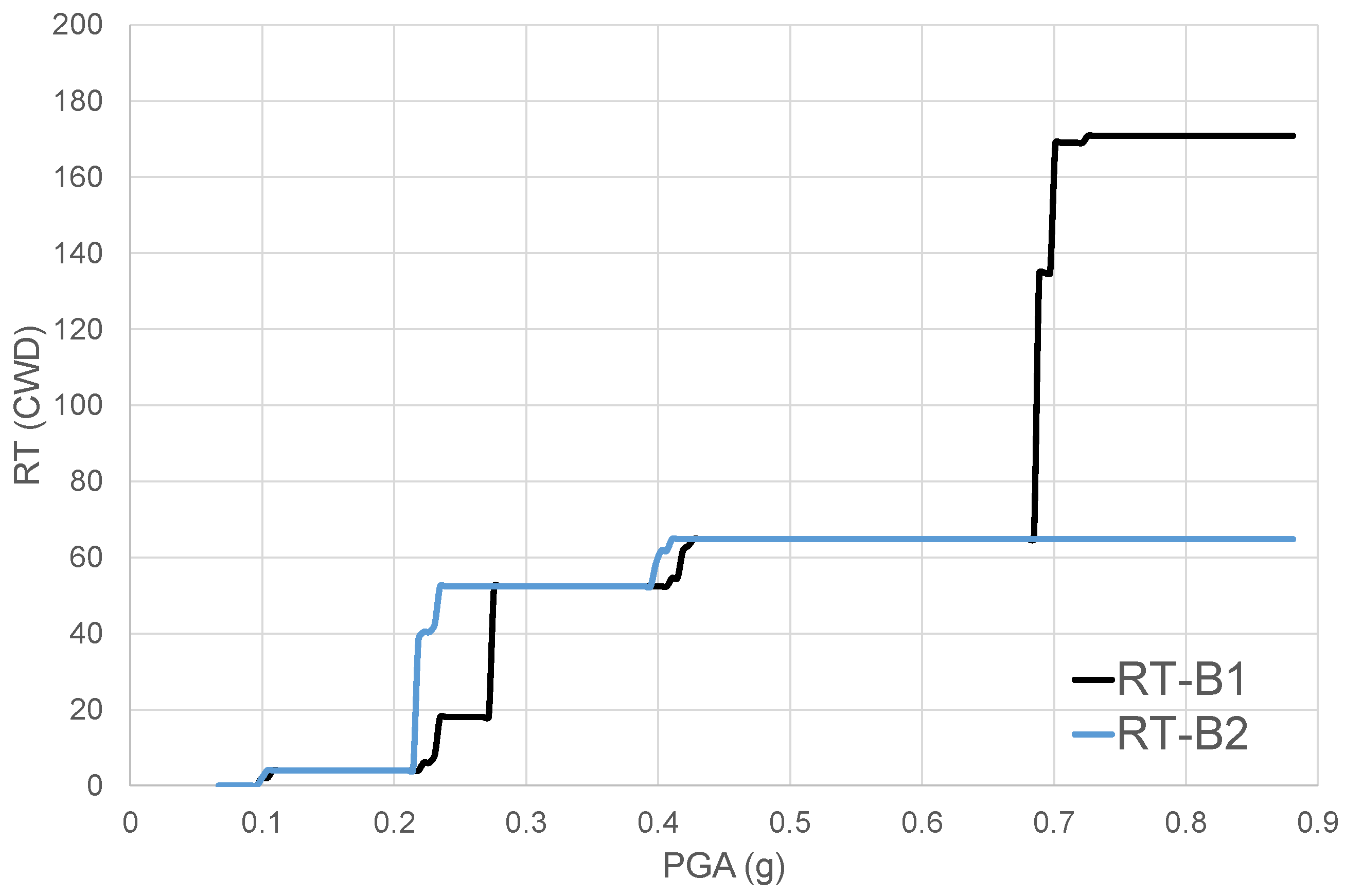
• RT is the repair time (RT) that is necessary to recover the original functionality;
• Q(t) is the recovery function that describes the recovery process necessary to return to the pre-earthquake level of functionality (see Figure 1). It is important to note that the recovery function starts at the time of occurrence (idle time neglected).

As described in [18], this function may be defined as follows:

$$Q\left(t\right)=\beta ·{(t-t_{0E})}^{\alpha }+Q_0$$

(2)

where α and β are two parameters that describe the recovery to the original functionality.

β is the ratio between the final functionality Q and the original functionality of the system before the earthquake.

α is the exponent of growth, which represents the rate of increase in the functionality after the earthquake. It depends on several factors, such as the level of preparedness of the community, the interdependencies amongst systems, and the state of the community and the surrounding region. In particular, the proposed formulation was chosen because it is based on a limited number of parameters (t_0E, β, α, and Q₀) and a mathematical structure (power function) that can realistically describe restoration procedures. In addition, Equation (2) allows flexibility in the calibration to cover various infrastructure typologies. The existing data are fundamental in order to calibrate the parameters to be consistent with the practical experience of multi-sectorial actors (i.e., infrastructure owners, transportation authorities, and public administrators).

In order to consider both sources of losses with a probabilistic-based approach based on the PBEE methodology, several contributions have been proposed [18,41]. The two sources of losses have been calculated by considering the repair cost ratio (RCR), representing the direct losses as a percentage of the construction cost and the repair time (RT), which is used here to derive the indirect losses. It is significant to note that the interdependencies are included in the calculation of CL to consider the interactions between the various infrastructures.

The previous approach [7] proposed to calculate the losses as the sum of the direct and indirect losses:

$$L\left(Im\right)=D\left(Im\right)+I\left(Im\right)$$

(3)

where:

• Im is the intensity measure used for the definition of the hazard;
• D(Im) are the direct losses as proportional as the sum of the RCR and of the repair time (RT) calculated by the PBEE methodology:

  $$D\left(Im\right)=RT·{\displaystyle \sum }_{i=1}^{n}RC{R}_i\left(Im\right)$$

  (4)
• I(Im) are the indirect losses, calculated as follows:

$$I\left(Im\right)={\displaystyle \sum }_{i=1}^n(1-r_i)·P{T}_i\left(Im\right)+{\displaystyle \prod }_{i=1}^n\left(1-r_i\right)·C{L}_i\left(Im\right)$$

(5)

where:

• n is the number of interdependent infrastructures that are present in the network;
• r_i is the functionality ratio of the infrastructure (r = 1 means that the infrastructure is fully operational, r = 0 means that the infrastructure is closed);
• PT_i are the losses connected with prolongation of travel (PT) for infrastructures i = 1…n:

  $$P{T}_i\left(Im\right)=p_i·R{T}_i$$

  (6)
• p_i is a parameter that needs to be calibrated to calculate the PT for infrastructure i;
• CL_i represents the losses connected with connectivity loss (CL) for infrastructures i = 1…n;

  $$C{L}_i\left(Im\right)=c_i·R{T}_i$$

  (7)
• c_i is a parameter that needs to be calibrated to calculate the PT for infrastructure i;

In particular, the second term of Equation (5) considers the interdependencies of the various infrastructures, and consists of the products of the various functionality ratios. It is worth noting that this term is zero when one infrastructure of the networks is open and, thus, fully operational (r = 1). This simplification allows us to consider that there is no loss in connection, since the open infrastructure can compensate for the closure of the others. For example, there may be a case where one bridge is open and another is closed, but the two bridges may connect different parts of a network, so the connectivity of the closed bridge cannot be substituted by the fact that the first one is functional. In addition, Equation (5) is a general formulation that depends on the definition of Im, which measures the intensity of the considered seismic hazard.

4. Case Study

In this section, a case study is presented to compare two road networks (Infrastructures 1 and 2) that link the same locations, called O (origin) and E (end), and are subjected to a selected seismic hazard. Both infrastructures are built with the same typology of bridge (named B1 and B2, respectively), and n1 and n2 are the numbers of the bridges for each one. PGA (peak ground acceleration) was chosen as the reference Im, because the two bridge models have different dynamic characteristics and, thus, it was necessary to adopt an Im that does not depend on the structural properties (such as modal shapes). Figure 2 shows the selected situation.

Several assumptions were made:

(a) Direct costs and indirect losses were calculated by considering the bridges that are present along the network (other losses due to other components were neglected);

(b) The two networks have the same initial traffic conditions.

Note that the infrastructures are interdependent (n = 2) and, thus, indirect losses (I) can be calculated as follows:

$$\mathrm{I}=\left(1-r_1\right)·n_1·p_1·R{T}_1+(1-r_2)·n_2·p_2·R{T}_2+\left(1-r_1\right)·(1-r_2)·\left[n_1·c_1·R{T}_1+n_2·c_2·R{T}_2\right]$$

(8)

where:

• n₁ and n₂ are the number of bridges for Infrastructure 1 and Infrastructure 2, respectively;
• r₁ and r₂ are the functionality ratios of Infrastructures 1 and 2, respectively.

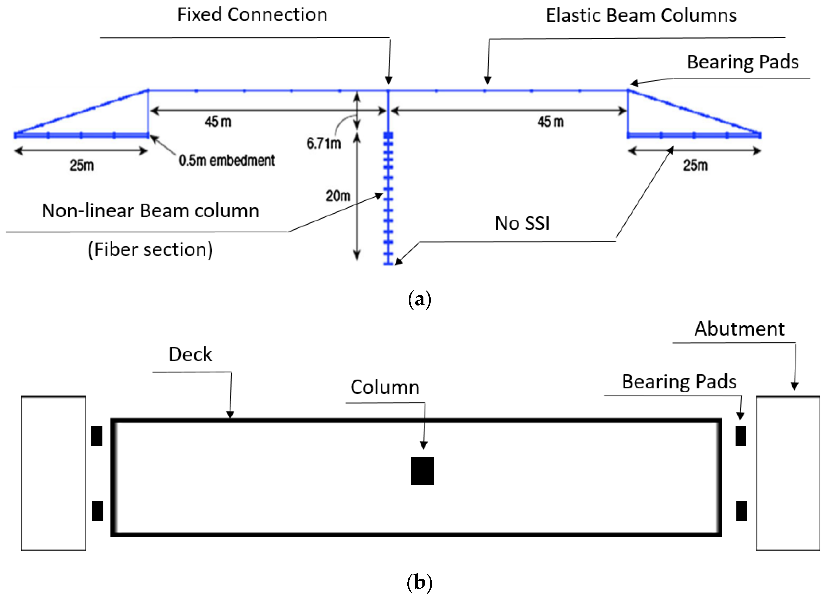
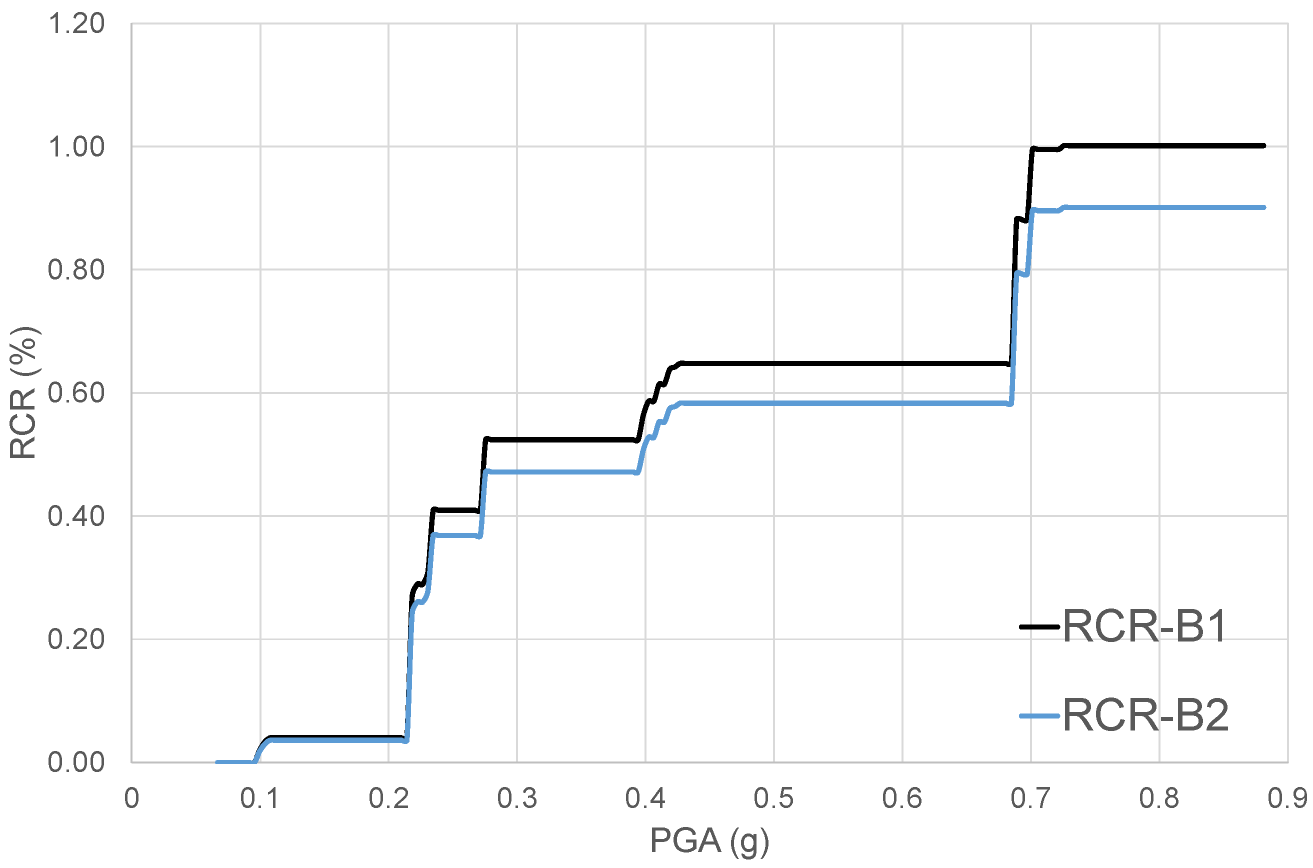
Note that the first and the second terms represent the contribution of PT, while the third term represents that of CL.

In the following text, several values of r₁ and r₂ are varied in order to explore several scenarios of PT, as shown in

Table 1. Various scenarios.

Scenario	r1	r2
n.1	0	1.0
n.2	0	0.5
n.3	0.5	0.5
n.4	0.5	0.75
n.5	0.5	1.0

. In particular, it is worth noting that in Scenarios 1 and 5, the second infrastructure can compensate for the closure of the first one.

4.1. Bridge Models

The bridges are two ordinary standard bridges (OSBs) representing California highway bridges, and designed according to the Caltrans Seismic Design Criteria [42], Figure 3a. The two benchmark bridges differ because of their longitudinal connections between the deck and the abutments, which are realized with different bearing pads in symmetrical positions, according to the plan locations (Figure 3b).

Bridge 1 (B1): The connections are realized with sliding isolators implemented with a simplified two-spring model, defined by the initial bending stiffness k1/2, yield strength Fy0, and post-yield stiffness k20 (28,500 kN/m, 287 kN, and 166.67 kN/m, respectively). More details may be found in [41,43,44].

Bridge 2 (B2): This scheme may move longitudinally because the connections between the deck and the abutments are achieved with soft damping rubber bearings. Such devices are modeled with two longitudinal elastic springs (730 kN/m) for each pad (modulus of elasticity G = 0.4 MPa and equivalent viscous damping n = 10%) [41].

In both bridges, the vertical and transversal directions of the abutments are restrained, and fixed connections are considered at the top of the column by restraining the translations and the rotations of the deck in all directions. The presence of the isolation allowed us to assume that the deck was capacity-designed; thus it was modeled with linear elastic beam–column elements (length: 90.00 m; width: 11.90 m; depth: 1.83 m; cross area: 5.72 m², transversal inertia: 2.81 m⁴ and vertical inertia: 53.9 m⁴, weight per unit length: 130.3 kN/m, as shown in

Table 2. Deck characteristics.

Characteristic
Length (m)	90.00
Width (m)	11.90
Depth (m)	1.83
E (MPa)	2.80 × 105
G (MPa)	1.15 × 105
Area (m2)	5.72
Itrasv (m4)	2.81
Ivert (m4)	53.9
Weight (kN/m)	130.3

). The 6.71 m RC column was represented with nonlinear fiber beam–column elements (see [45]) fixed at the base. Soil–structure interaction was also neglected, in correspondence with the connection between the soil and the approach ramps, which simulate the typical OSB concrete abutments (height: 6.71 m and length: 25 m) by assuming masses proportional to deck dead loads (to include the contribution of structural weight). The transversal direction of the bridge was constrained with rigid elements with a sufficiently high stiffness to be considered infinite, but allowing us to reproduce the rotation of the deck about the vertical axis [41].

4.2. SRRI Calculation

The Pacific Earthquake Engineering Research (PEER) Centre methodology, Ref. [31] was utilized to calculate the repair cost ratio (RCR) and recovery time (RT). The seismic scenario consisted of 100 input motions (from the PEER NGA database, http://peer.berkeley.edu/nga/, accessed on 15 August 2022) in order to reproduce typical California seismicity, as previously applied in [41]. Peak ground acceleration (PGA) was used as the reference intensity measure [31]. The losses were assessed by considering the Caltrans Comparative Bridge Costs database [42] and utilizing the LLRCAT methodology described in [33,35].

The results in terms of RCR (in %) and RT (in crew working days (CWD)) are shown in Figure 4 and Figure 5 for the two bridge configurations (B1 and B2). Figure 4 shows that at lower intensities, RCR is low and similar, while for PGA > 0.22 g, B1 has greater values than B2, and for PGA > 0.7 g, B1 reaches values of 1, meaning that the repair cost is the same as the complete reconstruction of the bridge.

Figure 5 shows the repair time that is necessary to return the individual bridges to their original functionalities. RT depends on the characteristics of the bridges, especially the adopted isolators. It is worth noting that the rate of RT is similar for many values of PGA. For the ranges 0.218 g–0.275 g and 0.402 g–0.427 g, B2 shows greater values of RT, with the maximum difference between 0.238 g and 0.275 g with RT values of 52.4 and 18.0, respectively, for Bridge 2 and Bridge 1. For these ranges of intensities, the sliders (model B1) seem to work better than rubber bearings. On the other hand, at the highest intensities (PGA > 0.684 g), the rubber bearings seem to perform better than the sliders. In particular, model B1 presents greater values than model B2, with maximum values of 171 CWD (corresponding to almost those times those associated with B2 (64.8 CWD)).

4.2.1. Case 1: n₁ = 3, n₂ = 6

Figure 6 shows the calculation of the losses (L) for the two infrastructures. Herein the case is that of two infrastructures with a different number of bridges (n₁ = 3 and n₂ = 6). It is possible to see that Scenario 2 is the worst, since Infrastructure 1 is totally closed and Infrastructure 2 can compensate for only 50% of the traffic flow. Comparing Scenario 1 and Scenario 5 shows the impact of the partial opening of the first infrastructure (Scenario 5) on losses, especially at medium intensities (reduction of around 50%) and at higher intensities (PGA > 0.68 g). Scenarios 3 and 4 represent cases where both of the infrastructures are damaged and, thus, partially opened. The results show that for PGA < 0.68 g, partially opening the two infrastructures (Scenario 3 and 4) incurs more losses than completely opening Infrastructure 2 (Scenario 1). For higher intensities (PGA > 0.68 g), Scenario 1 incurs more losses than Scenario 4.

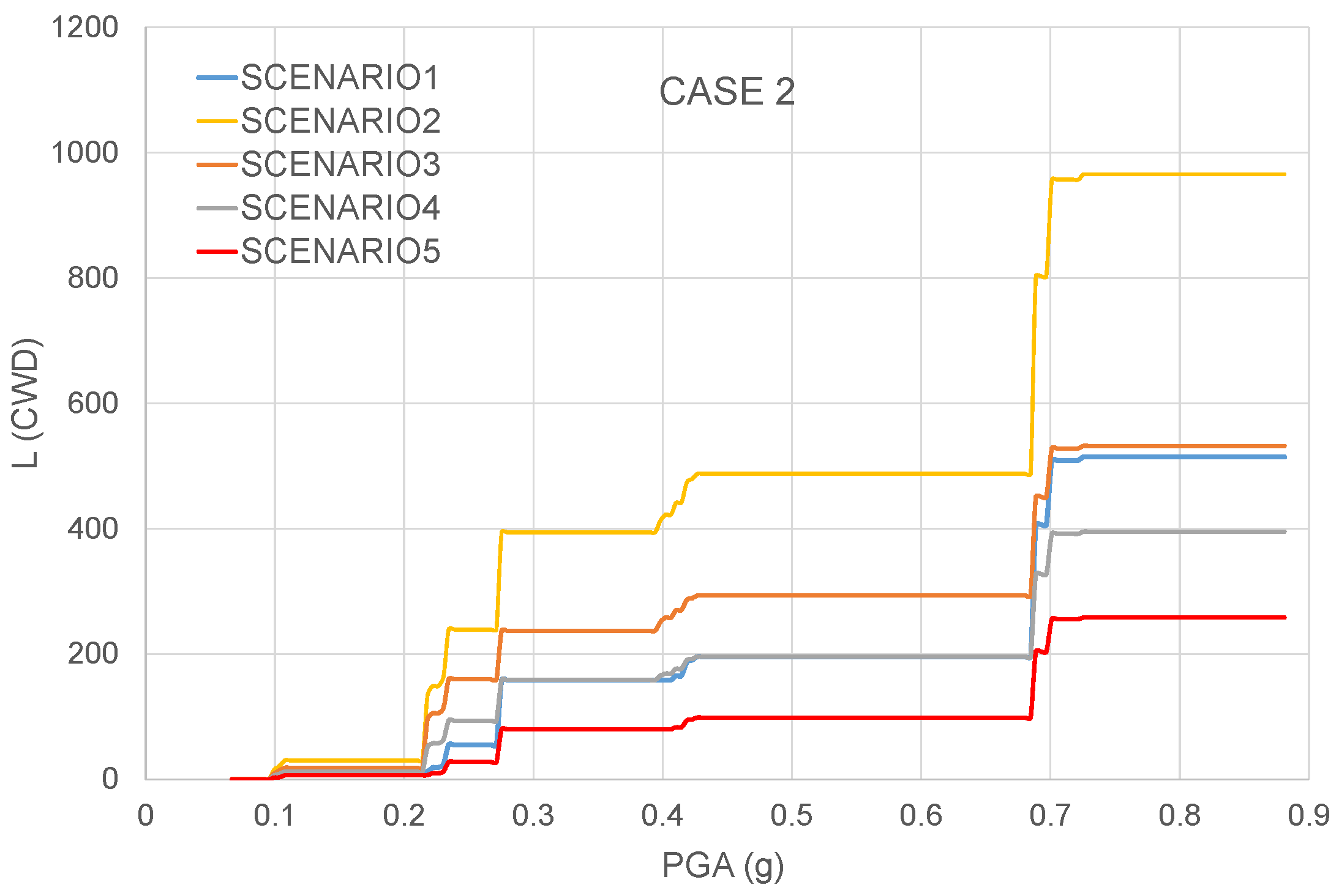
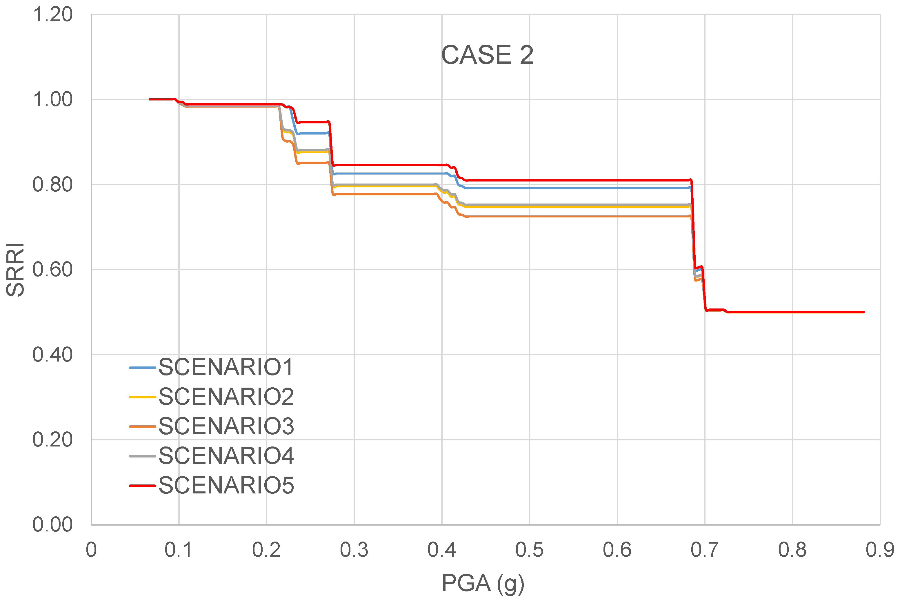
4.2.2. Case 2: n₁ = n₂ = 3

Figure 7 shows the calculation of the losses (L) for the two infrastructures in the event that the number of bridges is the same (n₁ = n₂ = 3) for the two infrastructures. It is possible to see that Scenario 2 is the worst and Scenario 5 is the best. The results show that for PGA < 0.68 g, Scenario 1 and Scenario 4 are similar. For PGA > 0.68 g, complete opening of Infrastructure 2 (Scenario 1) has the same effects as partial closures (Scenario 3), meaning that the results are intensity-dependent and, thus, that decision-makers need to carefully consider the earthquake hazard before taking decisions of full opening/partial opening/closure of the infrastructures.

4.2.3. SRRI Results

Figure 8 and Figure 9 show the SRRI results for the two cases and the five considered scenarios, with the following hypotheses: (1) The original functionality (at the time of occurrence of the earthquake) for both the infrastructures was 100%. (2) The applied repair functions were considered linear trends, as commonly assumed in the event of insufficient information. (3) The parameters c and p (Equations (5) and (6), respectively) were both considered to be 1, in order to consider both the prolongation of travel and losses connected with connection loss at the same level. These assumptions may be developed by improving the data from the characteristics of the road infrastructures. Figure 8 and Figure 9 show that for intensities between 0.21 g and 0.68 g, resilience depends on the different scenarios. The most resilient is Scenario 5, where the infrastructures are both opened (50% of Infrastructure 1 and 100% of Infrastructure 2). SRRI is shown to be minimal for Scenario 3, at all intensities.

Overall, the results demonstrate the validity of resilience as a parameter to define the state of road infrastructures after earthquakes. In particular, achieving a balance between resilient infrastructures and services is a duty for civil engineers in order to maintain post-earthquake functionality of communities. In this regard, a critical interpretation of SSRI results is fundamental for decision-makers in order to guarantee a minimal level of services for the infrastructures, adequate services and business for the communities, and rapid recoveries following seismic events.

5. Conclusions

The paper proposes a novel methodology to calculate the seismic resilience of road infrastructure by applying a performance-based approach for the computation of repair cost ratio and repair time. In this regard, the SRRI methodology considers both direct and indirect losses (i.e., prolongation of travel and connection losses), including the interdependencies between different infrastructures. Several case studies (10 cases: 2 bridges, 5 scenarios) were considered to apply the framework to realistic simulations. The ultimate goal of the proposed framework consists of assuming resilience as a valuable parameter to help in making decisions of full opening/partial opening/closure of the infrastructures. One limitation may be considered—the assessment of the role of soil–structure interaction (SSI), which may have important effects on the seismic resilience, as demonstrated in [8]. Such neglect does not compromise the high impact of the SRRI methodology due to uncertainties of soil and site effects [46].

References

1. Dehgani, M.; FLintsch, G.; McNeil, S. Impact of road conditions and disruption uncertainties on network vulnerability. J. Infrastruct. Syst. ASCE 2014, 20, 04014015. [Google Scholar] [CrossRef]
2. Moini, N. Modeling of Risks Threatening Critical Infrastructures: System Approach. J. Infrastruct. Syst. ASCE 2016, 22, 04015010. [Google Scholar] [CrossRef]
3. Nourzad, S.H.H.; Pradhan, A. Vulnerability of Infrastructure Systems. Macroscopic Analysis of Critical Disruptions on Road Networks. J. Infrastruct. Syst. ASCE 2016, 22, 04015014. [Google Scholar] [CrossRef]
4. Forcellini, D. A Resilience-Based (RB) Methodology to Assess Resilience of Health System Infrastructures to Epidemic Crisis. Appl. Sci. 2022, 12, 3032. [Google Scholar] [CrossRef]
5. Adey, B.; Hajdin, R.; Brudwile, E. Effect of common cause failures on indirect costs. J. Bridge Eng. 2004, 9, 200–208. [Google Scholar] [CrossRef]
6. Brookshire, D.S.; Chang, S.E.; Cochrane, H.; Olson, R.A.; Rose, A.; Steenson, J. Direct and indirect economic losses from earthquake damage. Earthq. Spectra. 1997, 14, 683–701. [Google Scholar] [CrossRef]
7. Forcellini, D. A new methodology to assess Indirect Losses in Bridges subjected to multiple hazards. Innov. Infrastruct. Solut. 2019, 4, 1–9. [Google Scholar] [CrossRef]
8. Forcellini, D. Resilience-Based Methodology to Assess Soil Structure Interaction on a Benchmark Bridge. Infrastructures 2020, 5, 90. [Google Scholar] [CrossRef]
9. Quang, C.; Shen, J.J.; Zhou, M.; Lee, G.C. Force-based and displacement-based reliability assessment approaches for highway bridges under multiple hazard actions. J. Traffic Transp. Eng. 2015, 2, 223–232. [Google Scholar]
10. Alipour, A.; Shafei, B.; Shinozuka, M. Reliability-based calibration of load and resistance factors for design of RC bridges under multiple extreme vents: Sour and earthquake. J. Bridge Eng. 2013, 18, 362–371. [Google Scholar] [CrossRef]
11. Gelh, P.; D’Ayala, D. Development of a Bayesian Networks for the multi-hazard fragility assessment of bridge systems. Struct. Saf. 2016, 60, 37–46. [Google Scholar] [CrossRef]
12. Andric, J.M.; Lu, D. Risk assessment of bridges under multiple hazards in operation period. Saf. Sci. 2016, 83, 80–92. [Google Scholar] [CrossRef]
13. Gardoni, P.; LaFave, J.M. Multi-hazard approaches to civil infrastructure engineering: Mitigating risks and promoting resilience. In Multi-Hazard Approaches to Civil Infrastructure Engineering; Gardoni, P., LaFave, J.M., Eds.; Springer: Berlin/Heidelberg, Germany, 2016; pp. 3–12. [Google Scholar]
14. Gidaris, I.; Padgett, J.E.; Barbosa, A.R.; Chen, S. Multiple-hazard fragility and restoration models of highway bridges for regional risk and resilience assessment in the United States: State-of-the-art review. J. Struct. Eng. 2017, 143, 04016188. [Google Scholar] [CrossRef]
15. Gautam, D.; Dong, Y. Multi-hazard vulnerability of structures and lifelines due to the 2015 Gorkha earthquake and 2017 central Nepal flash flood. J. Build. Eng. 2018, 17, 196–201. [Google Scholar] [CrossRef]
16. Chang, S.E.; Shinozuka, M. Measuring improvements in the disaster resilience of communities. Eng. Struct. 2004, 20, 739–755. [Google Scholar] [CrossRef]
17. Renschler, C.; Frazier, A.; Arendt, L.; Cimellaro, G.P.; Reinhorn, A.M.; Bruneau, M. Framework for Defining and Measuring Resilience at the Community Scale: The PEOPLES Resilience Framework; Technical Report MCEER-10-006; University at Buffalo: Buffalo, NY, USA, 2010. [Google Scholar]
18. Bruneau, M.; Chang, S.E.; Eguchi, R.T. A Framework to Quantitatively Assess and Enhance the Seismic Resilience of Communities. Earthq. Spectra 2003, 19, 733. [Google Scholar] [CrossRef]
19. Huang, Z.; Zhang, D.; Pitilakis, K.; Tsinidis, G.; Huang, H.; Zhang, D.; Argyroudis, S. Resilience assessment of tunnels: Framework and application for tunnels in alluvial deposits exposed to seismic hazard. Soil Dyn. Earthq. Eng. 2022, 162, 107456, ISSN 0267–7261. [Google Scholar] [CrossRef]
20. Mina, D.; Forcellini, D.; Karampour, H. Analytical fragility curves for assessment of the seismic vulnerability of HP/HT unburied subsea pipelines. Soil Dyn. Earthq. Eng. 2020, 137, 106308. [Google Scholar] [CrossRef]
21. Forcellini, D.; Walsh, K.Q. Seismic resilience for recovery investments of bridges methodology. In Proceedings of the Institution of Civil Engineers—Bridge Engineering; ICE Publishing: London, UK, 2021. [Google Scholar] [CrossRef]
22. Saydam, D.; Frangopol, D.M.; Dong, Y. Assessment of Risk Using Bridge Element Condition Ratings. J. Infrastruct. Syst. 2013, 19, 252–265. [Google Scholar] [CrossRef]
23. Ranjbar, P.R.; Naderpour, H. Probabilistic evaluation of seismic resilience for typical vital buildings in terms of vulnerability curves. Structures 2020, 23, 314–323. [Google Scholar] [CrossRef]
24. Argyroudis, S.A.; Nasiopoulos, G.; Mantadakis, N.; Mitoulis, S.A. Cost-based resilience assessment of bridges subjected to earthquake excitations including direct and indirect losses. Int. J. Disaster Resil. Built Environ. 2020, 12, 209–222. [Google Scholar] [CrossRef]
25. Meyer, V.; Becker, N.; Markantonis, V.; Schwarze, R.; van den Bergh, J.C.J.M.; Bouwer, L.M.; Bubeck, P.; Ciavola, P.; Genovese, E.; Green, C.; et al. Assessing the costs of natural hazards—State of the art and knowledge gaps. Nat. Hazards Earth Syst. Sci. 2013, 13, 1351–1373. [Google Scholar] [CrossRef]
26. Mechler, R.; Linnerooth-Bayer, J.; Peppiatt, D. Microinsurance for Natural Disasters in Developing Countries: Benefits, Limitations and Viability, ProVention Consortium, Geneva. 2006. Available online: http://www.proventionconsortium.org/themes/default/pdfs/Microinsurance study July06.pdf (accessed on 15 August 2022).
27. Hallegatte, S.; Dumas, P. Can Natural Disasters Have Positive Consequences? Investigating the Role of Embodied Technical Change. Ecol. Econom. 2008, 68, 777–786. [Google Scholar] [CrossRef]
28. Hallegatte, S.; Ghil, M. Natural Disasters Impacting a Macroeconomic Model with Endogenous Dynamics. Ecol. Econom. 2008, 68, 582–592. [Google Scholar] [CrossRef]
29. Hackl, J.; Adey, B.T.; Lethanh, N. Determination of Near-Optimal Restorationprograms for Transportation networks following Natural Hazard Events Using Simulated Annealing. Comput. -Aided Civ. Infrastruct. Eng. 2018, 33, 618–637. [Google Scholar] [CrossRef]
30. Mackie, K.R.; Wong, J.; Stojadinovic, B. Integrated Probabilistic Performance-Based Evaluation of Benchmark Reinforced Concrete Bridges; Report No. 2007/09; University of California Berkeley, Pacific Earthquake Engineering Research Center: Berkeley, CA, USA, 2008. [Google Scholar]
31. Mackie, K.R.; Wong, J.-M.; Stojadinovic, B. Post-earthquake bridge repair cost and repair time estimation methodology. Earthq. Eng. Struct. Dyn. 2010, 39, 281–301. [Google Scholar] [CrossRef]
32. Mackie, K.R.; Stojadinovic, B. Fourway: A graphical tool for performance-based earthquake engineering. J. Struct. Eng. 2006, 132, 1274–1283. [Google Scholar] [CrossRef]
33. Kröger, W.; Zio, E. Vulnerable Systems; Springer: London, UK, 2011. [Google Scholar] [CrossRef]
34. Rinaldi, S.M.; Peerenboom, J.P.; Kelly, T.K. Identifying, understanding, and analysing critical infrastructure interdependencies. In IEE Control Systems Magazine; IEEE: Piscataway, NJ, USA, 2001; pp. 11–25. Available online: http://user.it.uu.se/~bc/Art.pdf (accessed on 2 October 2012).
35. Ouyang, M. Review on modeling and simulation of interdependent critical infrastructure systems. Reliab. Eng. Syst. Saf. 2014, 121, 43–60. [Google Scholar] [CrossRef]
36. Adey, B.; Lethanh, N.; Lepert, P. An impact hierarchy for the evaluation of intervention strategies for public roads. In Proceedings of the 4th European Pavament Asset Management Conference (EPAM), Malmo, Sweden, 5–7 September 2012. [Google Scholar]
37. Luna, R.; Balakrishnan, N.; Dagli, C.H. Postearthquake recovery of a water distributionsystem: Discrete event simulation using colored Petri nets. J. Infrastruct. Syst. 2011, 17, 25–34. [Google Scholar] [CrossRef]
38. Grubesic, T.H.; Timothy, C.; Matisziw, T.C.; Murray, A.T.; Snediker, D. Comparative Approaches For Assessing Network Vulnerability. Int. Reg. Sci. Rev. 2008, 31, 88–112. [Google Scholar] [CrossRef]
39. Duenas-Osorio, L.; Craig, J.I.; Goodno, B.J. Seismic response of critical interdependent networks. Earthq. Eng. Struct. Dyn. 2007, 36, 285–306. [Google Scholar] [CrossRef]
40. Cimellaro, G.; Reinhorn, A.M.; Bruneau, M. Framework for analytical quantification of disaster resilience. Eng. Struct. 2010, 32, 3639–3649. [Google Scholar] [CrossRef]
41. Forcellini, D. Cost assessment of isolation technique applied to a benchmark bridge with soil structure interaction. Bull. Earthq. Eng. 2017, 15, 51–69. [Google Scholar] [CrossRef]
42. Caltrans (California Department of Transportation). Seismic Design Criteria Version 1.3; Caltrans: Sacramento, CA, USA, 2003. [Google Scholar]
43. Forcellini, D.; Kelly, J.M. The analysis of the large deformation stability of elastomeric bearings. J. Eng. Mech. ASCE 2014, 140, 04014036. [Google Scholar] [CrossRef]
44. Mazzoni, S.; McKenna, F.; Scott, M.H.; Fenves, G.L. Open System for Earthquake Engineering Simulation, User Command-Language Manual; OpenSees Version 2.0; Pacifc Earthquake Engineering Research Center, University of California: Berkeley, CA, USA, 2009. [Google Scholar]
45. Spacone, E.; Filippou, F.C.; Taucer, F. Fibre beam-column model for non-linear analysis of r/c frames: Part I. Formulation. Earthq. Eng. Struct. Dyn. 1996, 25, 711–725. [Google Scholar] [CrossRef]
46. Savvided, A.A.; Papadrakis, M. A computational study on the uncertainty quantification of failure of clays with a modified Cam-Clay yield criterion. SN Appl. Sci. 2021, 3, 659. [Google Scholar] [CrossRef]
Figure 1. Resilience calculation (L= losses; RT = repair time; Q = functionality).
Applsci 12 08945 g001
Figure 2. Scheme of the road infrastructures considered in the case study.
Applsci 12 08945 g002
Figure 3. (a) Benchmark bridges (vertical view). (b) Benchmark bridges (plan view).
Applsci 12 08945 g003
Figure 4. Repair cost ratio (%).
Applsci 12 08945 g004
Figure 5. Repair time (CWD).
Applsci 12 08945 g005
Figure 6. Case 1 (n1 = 3, n2 = 6).
Applsci 12 08945 g006
Figure 7. Case 2 (n1 = n2 = 3).
Applsci 12 08945 g007
Figure 8. SRRI: case 1 (n1 = 3, n2 = 6).
Applsci 12 08945 g008
Figure 9. SRRI: case 2 (n1 = n2 = 3).
Applsci 12 08945 g009