Analysis of Resonance Transition Periodic Orbits in the Circular Restricted Three-Body Problem

Abstract

Resonance transition periodic orbits exist in the chaotic regions where the 1:1 resonance overlaps with nearby interior or exterior resonances in the circular restricted three-body problem (CRTBP). The resonance transition periodic orbits have important applications for tour missions between the interior and the exterior regions of the system. In this work, following the increase of the mass parameter $\mu$ in the CRTBP model, we investigate the breakup of the first-order resonant periodic families and their recombination with the resonance transition periodic families. In this process, we can describe in detail how the 1:1 resonance gradually overlaps with nearby first-order resonances with increasing strength of the secondary’s perturbation. Utilizing the continuation method, features of the resonance transition periodic families are discussed and characterized. Finally, an efficient approach to finding these orbits is proposed and some example resonance transition periodic orbits in the Sun–Jupiter system are presented.

1. Introduction

Mean motion resonance (MMR) or orbital resonance is a common phenomenon both in our Solar system and the exoplanetary system that occurs when there is a ratio of integers between the orbital periods of two objects. For example, a resonance occurs between Neptune and Pluto (3:2 resonance) and Jupiter’s moons (1:2:4 resonance) in our Solar system. For MMRs in the exoplanetary system, numerous suspected or confirmed examples exist [1,2].

The resonant motions in the restricted three-body problem have been studied many times in the past years. The resonant periodic families and their stability corresponding to first-, second-, and other higher-order resonances in the CRTBP and the ERTBP model are reviewed by [3,4]. The transition between different resonances is also an interesting problem and has been investigated by many researchers. For example, Oterma, which is Jupiter’s comet, can make a rapid transition from the interior, near 3:2 resonance, to the exterior, near 2:3 resonance, with the secondary. This phenomenon of Oterma is called resonance hopping [5]. The dynamical mechanism of the resonance transition and capture of Jupiter’s comets is explained by [6,7,8]. Resonance transitions associated with the structure of the weak stability boundary are discussed in [9]. Furthermore, investigations about the resonance hopping effect are also conducted in the Neptune–Planet Nine system [10].

Recently, studies [11,12] examined the natural divergence of the first-order resonances for nearly circular orbits at low eccentricities. They indicate the existence of ‘bridges’ between adjacent first-order resonances at low eccentricities that smoothly connect the apocentric libration zone of a first-order resonance and the pericentric libration zone of the neighboring first-order resonance. This phenomenon is also present with the periodic orbits method in this work. Investigations of these bridges and gaps at low-eccentricity first-order resonance under dissipative effects are presented in [13]. In this paper, we conduct an investigation about the breakup of the first-order resonant periodic families by increasing the mass parameter $\mu$. In the chaotic region where the 1:1 resonance overlaps with nearby first-order resonances, specific periodic orbits with part of their trajectories resembling an interior/exterior resonant orbit and part of their trajectories resembling another interior/exterior resonant orbit are found, which are called the resonance transition periodic orbits (RTPOs). The breakup of the first-order resonance with the increasing mass parameter $\mu$ and recombination with the resonance transition periodic families (RTPFs) are introduced in this paper.

In recent years, the application of the resonance phenomenon has attracted much interest in engineering and mission design [14,15,16,17,18,19,20,21]. Practical missions using the resonant periodic orbits already exist. For example, in the extension phase of the IBEX (Interstellar Boundary Explorer) mission, the spacecraft was maneuvered into an orbit that is in the 3:1 resonance with the Moon [22,23]. Another mission is the TESS mission (Transiting Exoplanet Survey Satellite), which is in an orbit in the 2:1 resonance with the Moon [24,25]. By choosing a proper phase with the Moon, this resonant periodic orbit can minimize the radiation dose and avoid long eclipses to improve the efficiency of scientific work and sustain long-term stability. The resonant periodic orbits along with the RTPOs investigated in this work may have a wide application for tour missions in the Earth–Moon and other planetary systems in the future.

The remainder of this paper is structured as follows. In Section 2, the model framework is introduced. The structures of the first-order resonant periodic families are introduced in Section 3. The breakup and recombination process of the RTPFs with the first-order resonant periodic families are introduced in Section 4. Starting from unstable orbits in the 1:1 resonance region, an efficient approach to generating the symmetric RTPFs is proposed in Section 5. Section 6 concludes the study.

2. Model Framework

2.1. The CRTBP Model

The circular restricted three-body problem (CRTBP) model has been widely used to approximate the motions of small particles in the Solar system. In the CRTBP model, it is assumed that the two primaries ($P_1$ and $P_2$) have circular orbits about their common center of mass due to their mutual gravitational attraction. A massless particle P moves in the gravitational field generated by the two massive primaries: $P_1$ with mass $m_1$ and $P_2$ with mass $m_2$ [26]. The massless particle P has no influence on the movement of the two primaries. Usually, the dynamics of the CRTBP model are formulated in a rotating frame (synodic frame) and made non-dimensional by the following units:

$$\left[M\right]=m_1+m_2,\left[L\right]=a_{12},\left[T\right]=\sqrt{{\left[L\right]}^3/G\left[M\right]}$$

(1)

where $a_{12}$ is the mean distance of the two primaries. The unit of time $\left[T\right]$ is chosen such that the orbital period of $m_1$ and $m_2$ about their center of mass is $2\pi$. G is the gravitational constant. Equations of motion for P can be expressed as:

$$\ddot{\mathbf{r}}+2\left\{\begin{array}{c}-\dot{y}\\ \dot{x}\\ 0\end{array}\right\}={\left(\frac{\partial \mathrm{\Omega }}{\partial \mathbf{r}}\right)}^T$$

(2)

$$\mathrm{\Omega }=\frac{1}{2}\left[(x^2+y^2)+\mu (1-\mu )\right]+\frac{1-\mu }{r_1}+\frac{\mu }{r_2}$$

(3)

where $\mathbf{r}$ is the position vector ${[x,y,z]}^T$, and the dot indicates a derivative concerning the non-dimensional time of the rotating frame. $r_1$ and $r_2$ indicate the distance of P with respect to the barycenter of $P_1$ and $P_2$, respectively. The mass parameter $\mu$ is defined as $\mu =m_2/(m_1+m_2)$. In our studies, three systems, the unperturbed two-body (${\mu }_0$), the Sun–Earth (${\mu }_{SE}$), and the Sun = -Jupiter (${\mu }_{SJ}$) systems, are taken as specific examples to display the results. Their mass parameter values are shown in

Table 1. The mass parameter values of the unperturbed two-body system (${\mu }_0$), the Sun–Earth system (${\mu }_{SE}$), and the Sun–Jupiter (${\mu }_{SJ}$) system.

System/Name	Values
Two-body system (${\mu }_0$)	0
Sun–Earth system (${\mu }_{SE}$)	3.003480575402412 $\times {10}^{-6}$
Sun–Jupiter system (${\mu }_{SJ}$)	9.538811803631013 $\times {10}^{-4}$

. For the CRTBP model, there is an integral of motion in the form of

$$2\mathrm{\Omega }-({\dot{x}}^2+{\dot{y}}^2+{\dot{z}}^2)=\mathrm{C}$$

(4)

where $\mathrm{\Omega }$ is the gravitational potential and C is the Jacobi constant.

2.2. Periodic Orbits in the CRTBP Model

The CRTBP model is an autonomous dynamical system. In general, equations of motion (see Equation (2)) describing an autonomous system can be written as

$$\dot{\mathbf{X}}=F\left(\mathbf{X}\right)$$

(5)

where X denotes the state vector of the small particle P. The solution to this equation is

$$\mathbf{X}\left(t\right)=\mathrm{\Phi }({\mathbf{X}}_0,t)$$

(6)

where ${\mathbf{X}}_0$ is the initial state vector at the initial time $t_0=0$. The condition that a periodic orbit needs to satisfy is

$$\mathbf{X}({\mathbf{X}}_0,T)-{\mathbf{X}}_0=0$$

(7)

where T is the orbital period. To find a periodic orbit is to determine the initial state vector ${\mathbf{X}}_0$ and the period T that satisfy Equation (7). In total, Equation (7) has seven variables ($\mathbf{X}$ and T), which can be solved by the Newton–Raphson iteration method. Because of the existence of the Jacobi integral (see Equation (4)), only five out of the six equations in Equation (7) are independent. Therefore, we need to fix two variables out of the seven in Equation (7) when solving this equation. Once a solution, i.e., a periodic orbit of Equation (7), is obtained, the whole family of periodic orbits can be generated by the well-known predictor–corrector algorithm [27].

In this work, we focus on two types of periodic orbits in the CRTBP model. The first type of periodic orbit is the planar Lyapunov periodic orbit around the collinear libration points $L_1$ and $L_2$. Families of planar Lyapunov periodic orbits around $L_1$ and $L_2$ in the Sun–Earth system are shown as examples in Figure 1a,b, which have been extensively used by previous researchers. Details to compute these periodic orbits can be found in reference [26]. The second type of periodic orbit is the resonant periodic orbit. Orbital resonance is defined by the ratio p:q between the orbital periods, where p and q are incommensurable positive integers. Neglect the secondary’s gravity, i.e., treat the massless particle’s orbit around the primary as an unperturbed Keplerian orbit. We denote the orbital period of the massless particle P as $T_p$ and the secondary’s orbital period as $T_s$. A p:q resonant periodic orbit in the synodic frame should strictly satisfy [26,28]

$$\frac{T_s}{T_p}=\frac{p}{q}$$

(8)

When $p>q$ ($p<q$), the resonance is interior (exterior) resonance. Denote k as

$$k=|p-q|$$

(9)

in which $k\ge 0$, and k is the resonance order. In this work, $k=1$. One remark is that, in the CRTBP model, the orbital period of the massless particle does not exactly satisfy Equation (8) due to the secondary’s perturbation. Example orbits of the first-order interior resonant periodic orbits (3:2, 4:3, and 5:4 resonances), as well as the exterior resonant periodic orbits (2:3, 3:4, and 4:5 resonances) in the Sun–Earth system are presented in Figure 2.

3. The First-Order Resonant Periodic Families

3.1. The Unperturbed Two-Body Model: $\mu =0$

In the unperturbed two-body model, two different kinds of symmetric periodic orbits exist in the synodic frame [4,13,29,30]. The periodic orbits related to the circular orbits of the small body are called periodic orbits of the first kind, which belong to the circular family. The periodic orbits related to the elliptic orbits of the small body are called periodic orbits of the second kind, which belong to the resonant periodic family. In Figure 3, the relationships between the circular family and the interior/exterior first-order resonant periodic families are displayed in the $T-C$ plane; these are called characteristic curves and are used in previous literature [31,32,33]. For each first-order resonant periodic family, the characteristic curve in Figure 3 represents two branches: one corresponding to the perigee on the positive x-axis and the other to the apogee on the positive x-axis; i.e., they differ only in phase.

3.2. The CRTBP Model: $\mu >0$

With the increasing of the mass parameter $\mu$, research [31,32,34] indicates that the continuation of circular periodic families of the small body in the CRTBP model is possible in all cases except at the first-order interior resonance $(p+1)$:p and exterior resonance p:$(p+1)$, $p=1,2,3\dots$. In the CRTBP model, the two branches of each first-order resonant periodic family split in the $T-C$ plane. Example orbits in “Branch-I” (Type-I) and “Branch-II” (Type-II) of the interior 3:2, 4:3, and 5:4 resonances and the exterior 2:3, 3:4, and 4:5 resonances in the Sun–Earth system are presented in Figure 2. Recently, Pan and Hou [4] presented the genealogy of the first-order interior as well as exterior resonant periodic families in the $T-C$ plane for the Sun–Earth, Sun–Jupiter, and Earth–Moon systems. Studies indicate that the two branches of each first-order resonant periodic family split and combine with the near-circular branch to form a new family in the $T-C$ plane (see Figure 4a,b). This phenomenon is also verified in [11] using the Hamiltonian approach. More specifically, for the interior first-order resonances, the studies [4,11] indicate that starting from $p=1$, “Branch-II” of the $(p+1)$:p resonant periodic family and “Branch-I” of the $(p+2)$:$(p+1)$ resonant periodic family combine with part of the near-circular family to form a new periodic family. In the following, we call these new interior periodic families $IB\left(\right(p+1)-(p+2\left)\right)$, indicating that they are connecting the $(p+1)$:p resonant periodic family with the $(p+2)$:$(p+1)$ resonant periodic family. Similarly, starting from $p=2$, “Branch-I” of the exterior $(p-1)$:p resonant periodic family is recombined with “Branch-II” of the exterior p:$(p+1)$ resonant periodic family and part of the near-circular family to form a new periodic family. We denote this new family as family $OB(p-(p+1\left)\right)$ in this study. Details of the family $IB(3-4)$ and $OB(3-4)$ in the Sun–Earth system are presented in Figure 5a,b, respectively.

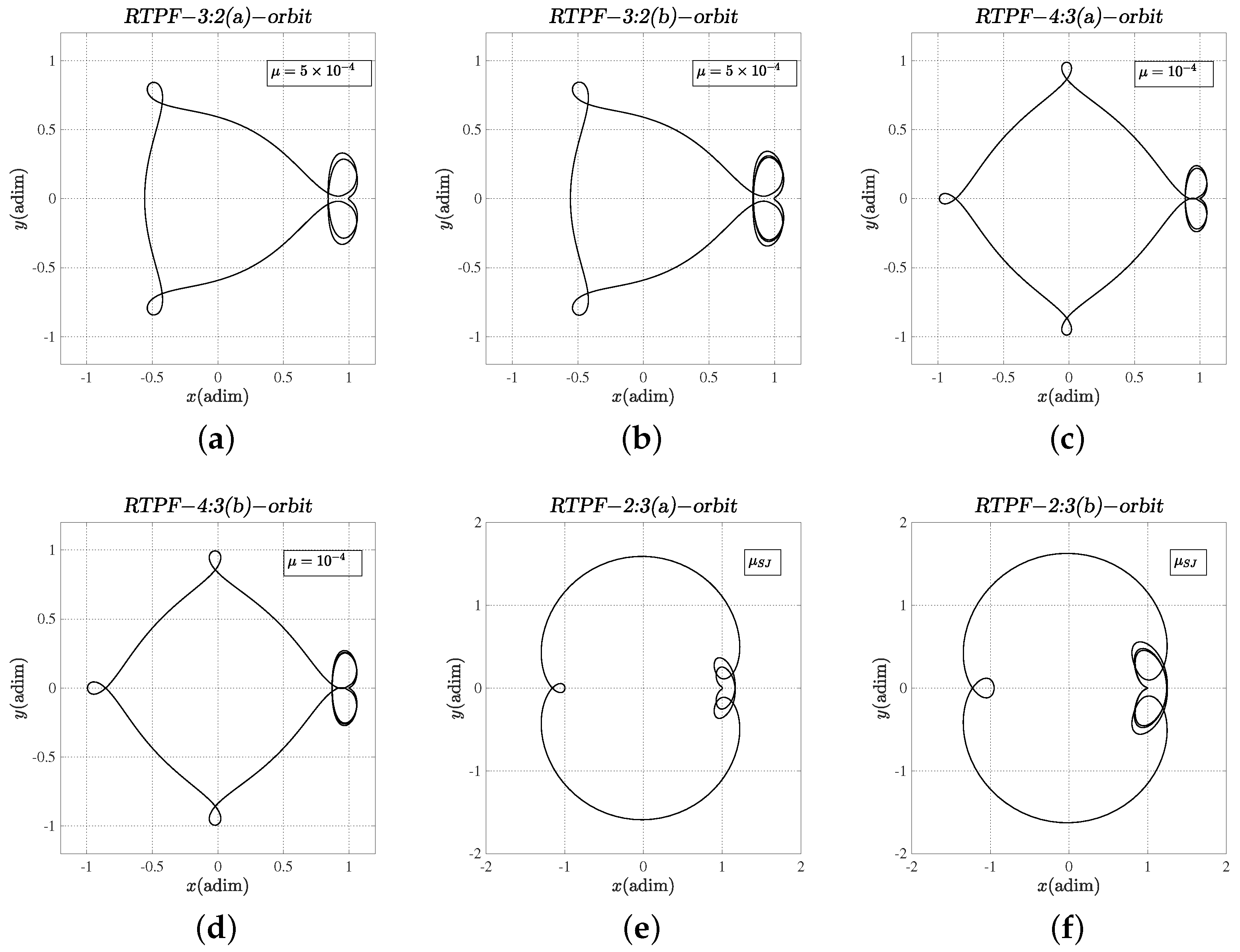
4. Resonance Transition Periodic Families in the CRTBP Model

In this work, we focus on the RTPFs in the CRTBP model. The RTPOs are the periodic orbits that connect the interior resonance and the exterior resonance by the 1:1 resonance. This kind of periodic orbit has similar orbital behavior to resonance hopping [5,7]. Here, we focus on how the 1:1 resonance overlaps nearby first-order resonances with increasing $\mu$. The breakup of the first-order resonant periodic families and their recombination with the RTPFs in the process of increasing the mass parameter $\mu$ are described as follows.

4.1. The RTPFs Related with the 3:2 Resonance

Even for very small $\mu \ne 0$, the RTPFs already exist, although they are not shown in the above characteristic curves of periodic families. In this section, we take the family $IB(3-4)$ as an example to show the process of family breakup and recombination with the RTPFs. This process can be viewed as the first-order resonances (here the 3:2 and the 4:3 ones) gradually being overlapped by the 1:1 resonance. In Figure 6, the family $IB(3-4)$ is continued from the Sun–Earth system to the Sun–Jupiter system, and characteristic curves of some example mass parameters are given. Comparing the characteristic curves in Figure 6a with Figure 5a, we can see that the genealogy of family $IB(3-4)$ becomes more complex and distorted with the increasing $\mu$.

Taking a closer look at the characteristic curves in Figure 6, we can see that there is no significant change of the family $IB(3-4)$ in the continuation process starting from the Sun–Earth system (${\mu }_{SE}$) to the system with $\mu ={10}^{-4}$. However, as the mass parameter further increases to $\mu =5\times {10}^{-4}$, noticeable changes in the characteristic curve occur in the $T-C$ plane. The changes are mainly reflected in two aspects: (1) for the branch near the 3:2 resonance, the characteristic curve bends as the Jacobi constant decreases, accompanied by the process of increasing, decreasing, and then increasing orbital period; (2) for the branch near the 4:3 resonance, the orbital period increases first, then decreases when it reaches a certain value, and finally continues to increase. The detailed characteristic curve of the family $IB(3-4)$ in the system with $\mu =5\times {10}^{-4}$ is separately presented by the orange line in Figure 7a. As the $\mu$ value further increases to $\mu ={\mu }_{SJ}$, a closed characteristic curve of family $IB(3-4)$ forms in the $T-C$ plane, which is represented by the red line in Figure 6 and Figure 7b.

In the process of increasing $\mu$ from $\mu =5\times {10}^{-4}$ to ${\mu }_{SJ}$, most family members of family $IB(3-4)$ in the system with $\mu =5\times {10}^{-4}$ still belong to the new family $IB(3-4)$ in the Sun–Jupiter system (${\mu }_{SJ}$). At the same time, small parts of the family $IB(3-4)$ in the system with $\mu =5\times {10}^{-4}$, especially for those close to the 3:2 resonance and the 4:3 resonance, combine with the RTPFs to form the new RTPFs in the Sun–Jupiter system. The bifurcation and recombination details are as follows. In the system with $\mu =5\times {10}^{-4}$, two RTPFs exist (see the green and purple line in Figure 7a). The green family is denoted as RTPF-3:2(a), and the purple family is denoted as RTPF-3:2(b). Example orbits in these two families are shown in Figure 11a,b, respectively. The RTPF-3:2(a) combines with some family members in “Branch-II” of the 3:2 resonance to form a new RTPF-3:2(a) in the Sun–Jupiter system (see the green line in Figure 7b). Similarly, the RTPF-3:2(b) combines with some family members in “Branch-I” of the 4:3 resonance to form a new RTPF-3:2(b) in the Sun–Jupiter system (see the purple line in Figure 7b). The shapes of the orbits in RTPF-3:2(a) and RTPF-3:2(b) are similar. Both of them have four apogees in the synodic frame, two of which are near the collinear libration point $L_1$. From the shape of the example RTPOs in Figure 11a,b, we know that part of the orbits around the collinear $L_1$ point resembles the planar Lyapunov periodic orbits (see Figure 1a), and part of the orbits far away from the collinear point resembles the 3:2 resonant orbit shown in Figure 2a (type-II). In addition, the characteristic curves of RTPF-3:2(a) and RTPF-3:2(b) (see the green and purple line in Figure 7) indicate that the difference in Jacobi constants between these two RTPFs is not significant. Orbits in the two RTPFs are different due to the difference in the number of revolutions around the libration point $L_1$ (RTPF-3:2(a): two revolutions; RTPF-3:2(b): three revolutions), which can be seen from Figure 11a,b.

4.2. The RTPFs Related with the 4:3 Resonance

Similar to the family $IB(3-4)$ which connects the 3:2 resonance to the 4:3 resonance, the family $IB(4-5)$ also has three components: (1) “Branch-II” of the 4:3 resonance, (2) “Branch-I” of the 5:4 resonance, and (3) the branch of the near-circular family. We continue the family $IB(4-5)$ from the Sun–Earth system to the Sun–Jupiter system. A similar breakup and recombination process happens during the process of increasing $\mu$.

Characteristic curves of some mass parameters during the process of increasing $\mu$ from the Sun–Earth system (${\mu }_{SE}$) to the Sun–Jupiter system (${\mu }_{SJ}$) are displayed in Figure 8. In the $T-C$ as well as the $x_0-C$ plane, the characteristic curves of the family $IB(4-5)$ have no significant change from the Sun–Earth system to the system with $\mu =5\times {10}^{-5}$. However, when the mass parameter further increases to $\mu ={10}^{-4}$, noticeable changes of the characteristic curve occur in the $T-C$ plane in two ways: (1) for the branch near the 4:3 resonance, the characteristic curve bends as the Jacobi constant decreases, accompanied with the process of increasing, decreasing, and then increasing orbital period; (2) for the branch near the 5:4 resonance, the orbital period increases first, then decreases when it reaches a certain value, and finally continues to increase. The characteristic curve of the family $IB(4-5)$ for the system with $\mu ={10}^{-4}$ is separately represented by the yellow line in Figure 9a. Similarly, the branches near the 4:3 resonance and the 5:4 resonance come closer to each other with the increasing $\mu$. Different from the case of the family $IB(3-4)$, a closed characteristic curve of the family $IB(4-5)$ already forms in the $T-C$ plane as the $\mu$ value increases to $\mu =5\times {10}^{-4}$. This means the breakup and recombination of the family $IB(4-5)$ happens for smaller $\mu$ values when compared with the family $IB(3-4)$. When the mass parameter further increases to ${\mu }_{SJ}$, the size of the closed curve becomes smaller, which is represented by the red line in Figure 9b.

In the process of mass parameter continuation from $\mu ={10}^{-4}$ to ${\mu }_{SJ}$, most family members of the family $IB(4-5)$ in the system with $\mu ={10}^{-4}$ still belong to the new family $IB(4-5)$ in the Sun–Jupiter system (${\mu }_{SJ}$). At the same time, small parts of the family $IB(4-5)$ in the system with $\mu =5\times {10}^{-4}$, especially for those close to the 4:3 resonance and the 5:4 resonance, combine with the RTPFs to form the new RTPFs in the Sun–Jupiter system. Two RTPFs work in the bifurcation and recombination process, which are denoted as RTPF-4:3(a) and RTPF-4:3(b) (see the green and purple line in Figure 9a). The RTPF-4:3(a) combines with some family members in “Branch-II” of the 4:3 resonance to form a new RTPF-4:3(a) in the Sun–Jupiter system (see the green line in Figure 9b). Similarly, the RTPF-4:3(b) combines with some family members in “Branch-I” of the 5:4 resonance to form a new RTPF-4:3(b)) in the Sun–Jupiter system (see the purple line in Figure 9b). Example orbits from the RTPF-4:3(a) and the RTPF-4:3(b) are presented in Figure 11c,d, respectively. The shapes of the orbits in RTPF-4:3(a) and the RTPF-4:3(b) are similar. Both of them have five apogees in the synodic frame, two of which are near the collinear libration point $L_1$. Part of the orbits close to the collinear libration point resembles the planar Lyapunov periodic orbits around the $L_1$ point and the remaining part of the orbits resembles the 4:3 resonant periodic orbits (see the Type-II in Figure 2b). In addition, characteristic curves (see the green and purple line in Figure 9) of the RTPF-4:3(a) and RTPF-4:3(b) indicate that the difference in Jacobi constants between these two RTPFs is not significant. Orbits in the RTPF-4:3(a) and the RTPF-4:3(b) are different due to the difference in the number of revolutions near the libration point $L_1$ (RTPF-4:3(a): two revolutions; RTPF-4:3(b): three revolutions), which can be seen from the example orbits in Figure 11c,d.

4.3. The RTPFs Related with the 2:3 Resonance

The exterior first-order resonant periodic families have similar breakup and recombination processes as the interior resonances during the process of increasing $\mu$. Taking the family $OB(3-4)$ as an example, the breakup and recombination process with the RTPFs are as follows. The family $OB(3-4)$ in the CRTBP model has three components: (1) “Branch-I” of the 2:3 resonance, (2) “Branch-II” of the 3:4 resonance, and (3) the branch of the near-circular family (see Figure 5b). We continue the family $OB(3-4)$ from the Sun–Earth system to the Sun–Jupiter system. Characteristic curves of some mass parameters during the process of increasing $\mu$ from the Sun–Earth system (${\mu }_{SE}$) to the Sun–Jupiter system (${\mu }_{SJ}$) are displayed in the $T-C$ plane (see Figure 10a). Similarly, when the mass parameter is small (from the Sun–Earth system to the system with $\mu =5\times {10}^{-5}$), there are no significant changes in the characteristic curves. However, when the mass parameter further increases to $\mu ={10}^{-4}$, noticeable changes of the characteristic curve occur in the $T-C$ plane in two ways: (1) for the branch near the 2:3 resonance, the characteristic curve bends as the Jacobi constant decreases, accompanied with the process of increasing, decreasing, and then increasing orbital period; (2) for the branch near the 3:4 resonance, the orbital period increases first, then decreases when it reaches a certain value, and finally continues to increase. A closed characteristic curve of family $OB(3-4)$ forms when $\mu =5\times {10}^{-4}$ (see the orange line in Figure 10a). When the mass parameter further increases to ${\mu }_{SJ}$, the size of the closed curve becomes smaller, which is represented by the red line in Figure 10.

With the increasing mass parameter $\mu$, most family members of the family $OB(3-4)$ in the system with $\mu ={10}^{-4}$ still belong to the new family $OB(3-4)$ in the Sun–Jupiter system (${\mu }_{SJ}$). At the same time, small parts of the family $OB(3-4)$ in the system with $\mu ={10}^{-4}$, especially for those close to the 2:3 resonance and the 3:4 resonance, combine with the RTPFs to form the new RTPFs in the Sun–Jupiter system. Two RTPFs work in the bifurcation and recombination process, which are denoted as RTPF-2:3(a) and RTPF-2:3(b). RTPF-2:3(a) combines with some family members in “Branch-I” of the 2:3 resonance to form a new RTPF-2:3(a) in the Sun–Jupiter system (see the green line in Figure 10b). Similarly, RTPF-2:3(b) combines with some family members in “Branch-II” of the 3:4 resonance to form a new RTPF-2:3(b)) in the Sun–Jupiter system (see the purple line in Figure 10b). Example orbits from RTPF-2:3(a) and RTPF-2:3(b) in the Sun–Jupiter system are presented in Figure 11e,f, respectively. The shapes of the orbits in RTPF-2:3(a) and the RTPF-2:3(b) are similar. Both of them have three perigees in the synodic frame, two of which are near the collinear libration point $L_2$ (see Figure 1b). Part of the orbits close to the collinear libration point resembles the planar Lyapunov periodic orbits around the $L_2$ point and the remaining part of the orbits resembles the 2:3 resonant periodic orbits (see Figure 2d (Type-I)). In addition, characteristic curves of the two RTPFs in Figure 10b (see the green and purple line) indicate that the difference in Jacobi constants between these two RTPFs is not significant. Orbits in the two RTPFs are different due to the difference in the number of revolutions around the libration point $L_2$ (RTPF-2:3(a): two revolutions; RTPF-2:3(b): three revolutions), which can be seen from Figure 11e,f.

4.4. Summation

In the CRTBP model, the families $IB(p-(p+1\left)\right)$ connect the “Branch-II” of the interior p:$(p-1)$ resonance with the “Branch-I” of the interior $(p+1)$:p resonance. The families $OB(p-(p+1\left)\right)$ connect the “Branch-I” of the exterior $(p-1)$:p resonance with the “Branch-II” of the exterior p:$(p+1)$ resonance. This genealogy of the periodic families has already been pointed out by some previous studies [4,11,31,32].

With the mass parameter $\mu$ increasing, starting from larger values of p, the first-order resonant periodic families $IB(p-(p+1\left)\right)$ and $OB(p-(p+1\left)\right)$ gradually disappear because they are overlapped by the 1:1 resonance. The RTPOs have part of the orbit resembling the planar Lyapunov orbits around the $L_1$ or $L_2$ point, and the other part resembling the interior or exterior resonant periodic orbits. The collinear libration points along with the orbits around them can be taken as unstable ’saddle points’ of the 1:1 resonance. As a result, the RTPOs can be taken as the connection orbits between the 1:1 resonance region and the interior or the exterior resonance regions. By following the breakup and recombination process of the families $IB(p-(p+1\left)\right)$ and $OB(p-(p+1\left)\right)$ with the RTPFs, the details of the resonance overlapping process are revealed by the approach of periodic orbits.

5. Computation of the Symmetric RTPOs

According to the studies above, we know that the strength of the 1:1 resonance increases with the increasing $\mu$. It gradually overlaps with nearby interior or exterior resonances, leading to chaos in these overlapped regions. During this process, the RTPFs play a fundamental role in connecting the 1:1 resonance with the interior or the exterior resonances. The RTPOs presented above have part of their orbits resembling the collinear libration point orbits and the remaining part of the orbits resembling the interior or the exterior resonances. Generally, the regions overlapped by the 1:1 resonance are chaotic. There are also RTPOs connecting both the interior and the exterior resonances, through the orbits around $L_1$ or the $L_2$ points. In this section, we propose an efficient way to generate the symmetric RTPOs, and some examples in the Sun–Jupiter system are given.

5.1. Methodology

• Firstly, we restrict the starting position on the Lyapunov orbit around the collinear $L_1$ or $L_2$ point in the Sun–Jupiter system and extend the method in the previous study [35] to the Sun–Jupiter system. The amplitude of the Lyapunov orbit is defined as the distance between its right intersection point (see the yellow dot in Figure 12) with the x-axis and the $L_1$ or the $L_2$ point. In our work, it is fixed at 0.05 (dimensionless unit) of the Sun–Jupiter distance. One remark is that a different value can be chosen. Initial states of the planar Lyapunov orbit are denoted as $(x_0,y_0,0,\dot{x_0},\dot{y_0},0)$. The Lyapunov orbit is symmetric about the x-axis. The initial position is placed on the positive x-axis and the initial velocity is exactly along the positive y-direction. Therefore, the initial state of the Lyapunov orbit is $(x_0,0,0,0,\dot{y_0},0)$;
• We add a tiny perturbation $\mathrm{\Delta }v$ along the direction of initial velocity ${\dot{y}}_0$ on the Lyapunov orbit. The velocity change $\mathrm{\Delta }v$ is in the range of [−0.01, 0.01] in this study, i.e., the departure velocity ${\dot{y}}_d$ at the initial position is restricted to be within [−0.01 + ${\dot{y}}_0$, 0.01 + ${\dot{y}}_0$], where 0.01 is a dimensionless velocity in the Sun–Jupiter system. Due to the linear stability of the collinear libration point, the orbit can leave the vicinity of the collinear libration point with this tiny perturbation to the initial velocity. The schematic diagram of generating initials of the RTPOs is displayed in Figure 12;
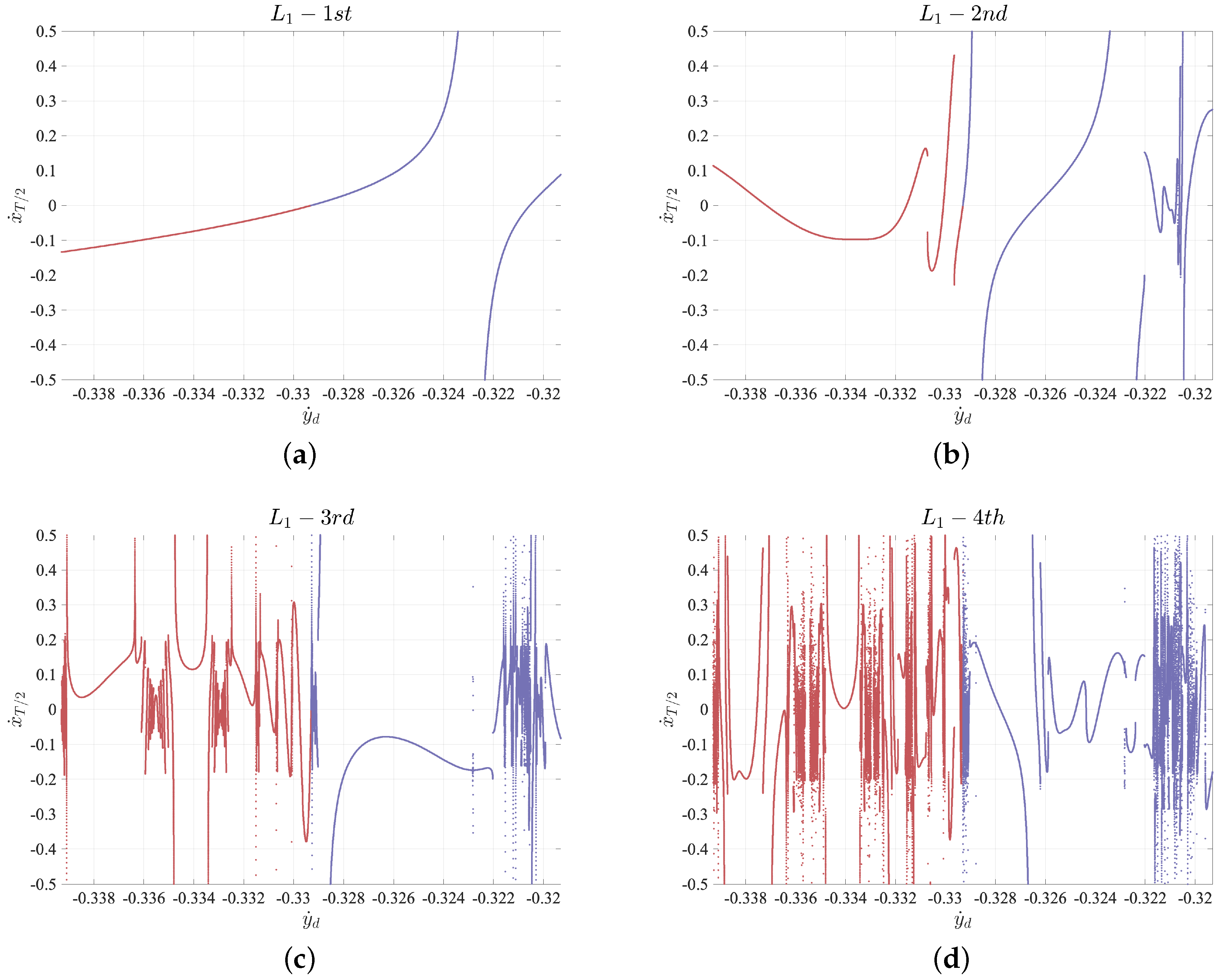
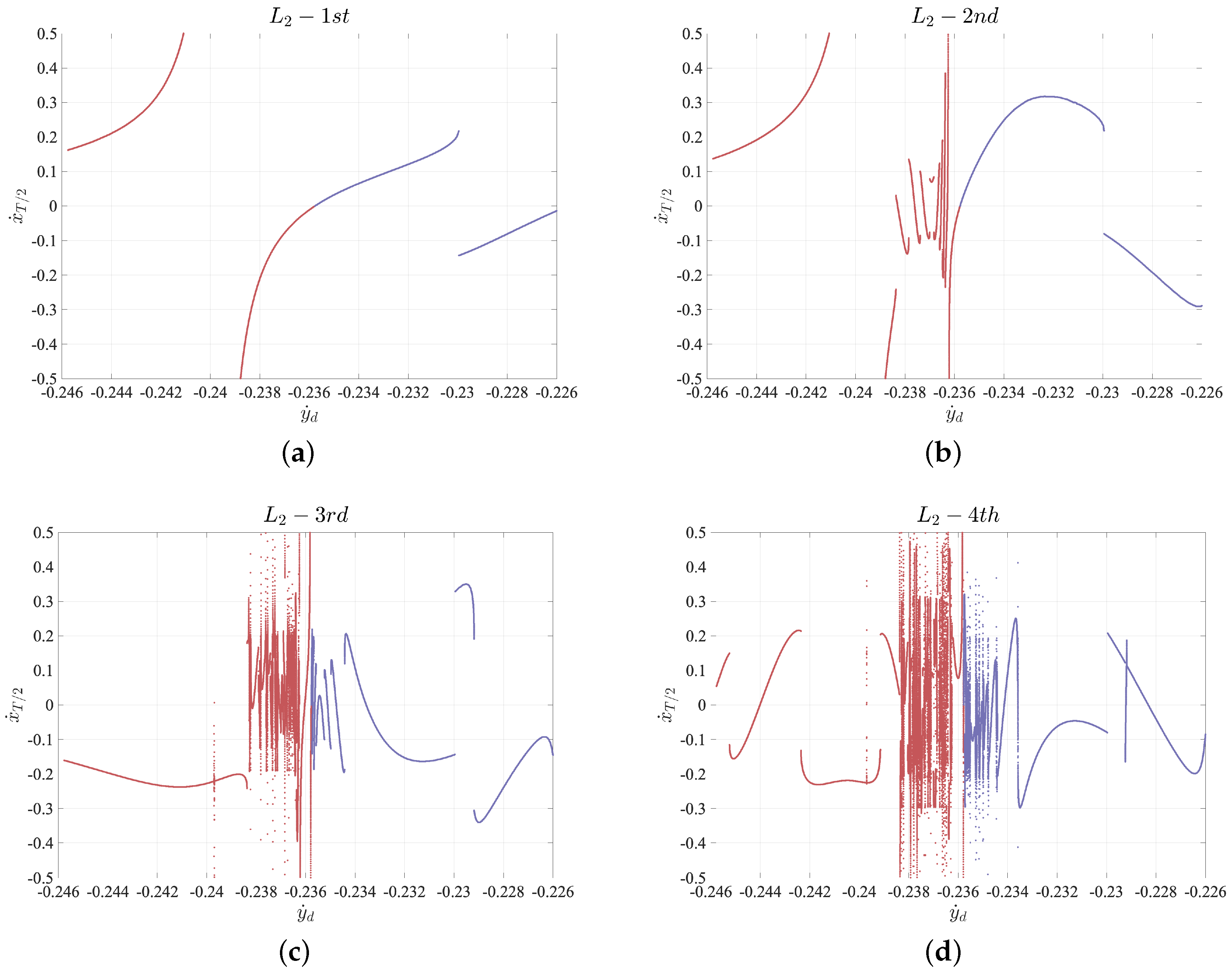
• By integration, the trajectory leaves the initial position on the x-axis. If the initial velocity ${\dot{y}}_d$ is appropriate, it crosses the x-axis again one or more times after some integration time. Generally, at the new intersection point (see the green point in Figure 12), the velocity is not perpendicular to the x-axis. We record the x component of the velocity at the new intersection point and denote it as ${\dot{x}}_{T/2}$. For a different value of the departure velocity ${\dot{y}}_d$, the value of ${\dot{x}}_{T/2}$ is different. By varying the values of ${\dot{y}}_d\in [-0.01+{\dot{y}}_0,0.01+{\dot{y}}_0]$ and the times of the trajectory intersects with the x-axis after departure, the relationships between ${\dot{x}}_{T/2}$ and ${\dot{y}}_d$ are obtained;
• The relationships between ${\dot{x}}_{T/2}$ and ${\dot{y}}_d$ are presented in Figure 13 (cases for $L_1$) and Figure 14 (cases for $L_2$). According to the well-known symmetry property of the CRTBP model $(x,y,z,\dot{x},\dot{y},\dot{z},t)\leftarrow \to (x,-y,z,-\dot{x},\dot{y},-\dot{z},-t)$ [26], if ${\dot{x}}_{T/2}=0$, the trajectory from $t=0$ to $t=T/2$ is half of a periodic orbit. From Figure 13 and Figure 14, we can see that there exist some dots satisfying ${\dot{x}}_{T/2}\approx 0$ within a certain tolerance, which means that we can use these initial states $(x_0,0,0,0,{\dot{y}}_d,0)$ where ${\dot{x}}_{T/2}\approx 0$ to generate the periodic orbits, especially for the RTPOs. After finding these initial states $(x_0,0,0,0,{\dot{y}}_d,0)$, we can use the Newton iteration method to find the exact initial velocity ${\dot{y}}_d$ that makes ${\dot{x}}_{T/2}=0$. The same algorithm has been used to generate the symmetric horseshoe periodic orbits in the CRTBP model [33,36].

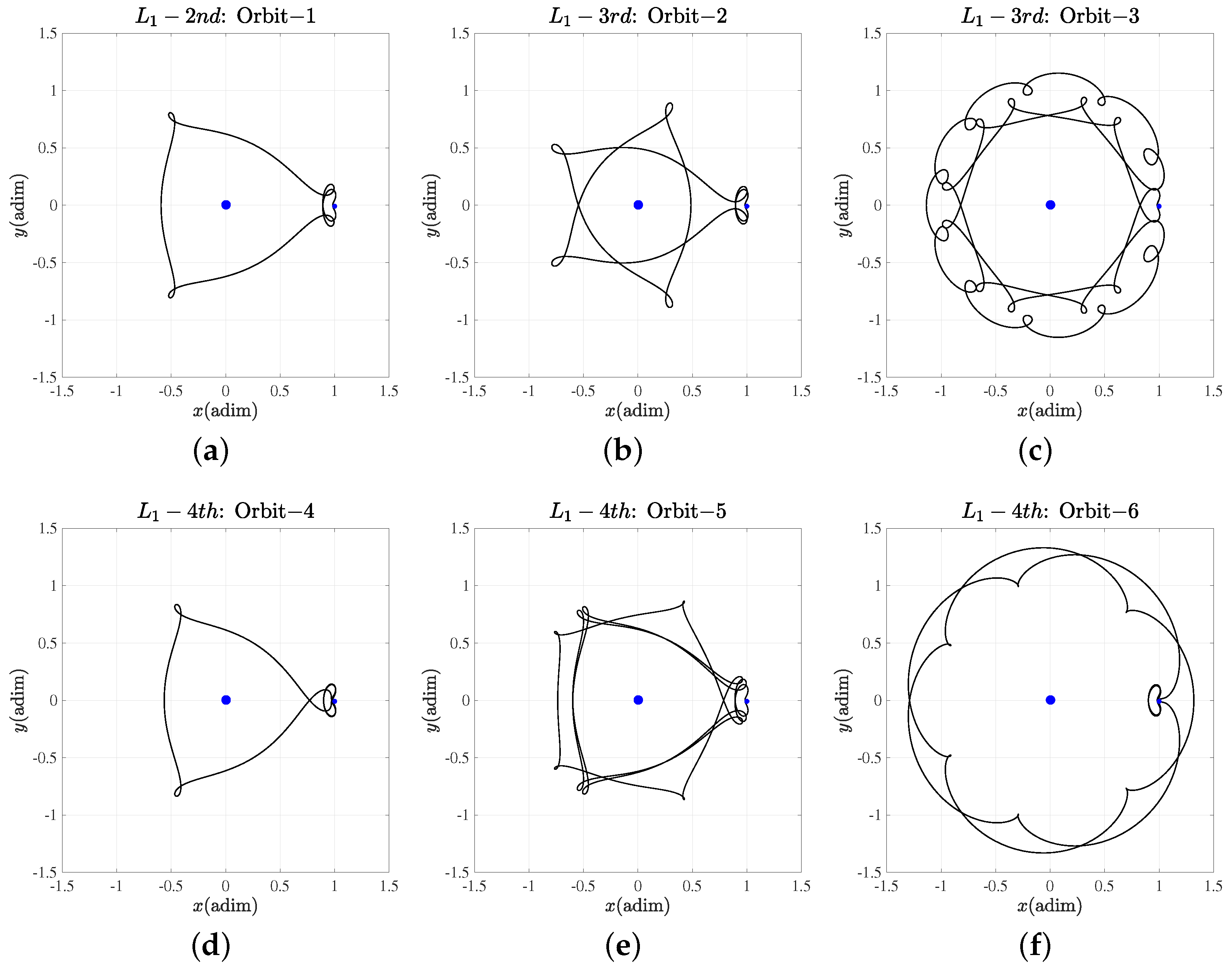
5.2. Results

Similar to the computation of the resonant periodic families in the above sections, once a RTPO is found, the whole family can be generated by the predict–correct algorithm. In this section, we limit ourselves to the computation of specific RTPOs, but not the families. Some example orbits are given below.

Examples of the RTPOs related to $L_1$ as well as $L_2$ are given in Figure 15 and Figure 16, respectively. In Figure 15, six RTPOs related to $L_1$ are presented, including (1) a resonance transition between the 1:1 resonance and other resonances (Orbit-1, Orbit-2, and Orbit-4); (2) a resonance transition between the interior and exterior resonances by the 1:1 resonance (Orbit-3); (3) a resonance transition between two interior resonances with the aid of 1:1 resonance (Orbit-5); (4) a resonance transition between two exterior resonances by the 1:1 resonance (Orbit-6). Similarly, six examples of the RTPOs corresponding to $L_2$ are displayed in Figure 16, which correspond to (1) a resonance transition between the 1:1 and other resonances (Orbit-1, Orbit-2, and Orbit-3); (2) a resonance transition between the interior and exterior resonances by the 1:1 resonance (Orbit-4); (3) a resonance transition between two exterior resonances with the aid of 1:1 resonance (Orbit-5 and Orbit-6).

The RTPOs can stay around $L_1$ or $L_2$ for one or more loops before leaving to other resonances. This feature shows that the RTPOs are suitable for missions requiring long-term continuous observations of the second primary. The transition between different resonances by the 1:1 resonance indicates that the RTPOs can be applied to trajectory design for tour missions of the interior and exterior regions of the system. Various RTPOs emanating from the same generating orbit of $L_1$ or $L_2$ indicate that the spacecraft can transfer from one RTPO to another by performing a small maneuver in the vicinity of the generating orbit, which may significantly increase the flexibility of the mission design [18]. In our study, the RTPOs are unstable; therefore, station-keeping maneuvers are required if they are applied to practical missions.

6. Conclusions

In summary, details of the breakup and recombination of the interior as well as the exterior resonant periodic families with the RTPFs are revealed in this work with increasing $\mu$. Starting from the first-order resonant periodic families in the Sun–Earth system, we gradually increase the mass parameter $\mu$ to the Sun–Jupiter systems. In the process of continuing these periodic families, we observe the gradual changes in the phase space structure of the first-order resonance due to the increasing perturbation strength from the secondary in the CRTBP model. Two phenomena are reported. (1) With the mass parameter $\mu$ increasing, the strength of the 1:1 resonance becomes stronger. Starting from large values of p, the interior $(p+1)$:p and the exterior p:$(p+1)$ resonances are gradually overlapped by the 1:1 resonance, in a way that the characteristic curves of these resonance periodic families break up, recombine, and finally disappear. (2) Resonance transition periodic orbits connecting the 1:1 resonance and the interior/exterior resonances appear, forming the bridge connecting the 1:1 resonance region with the interior/exterior resonances. Their appearance indicates that the resonances are already obviously influenced by the 1:1 resonance. Furthermore, starting from the planar Lyapunov orbits in the 1:1 resonance region, we propose an efficient way to compute the symmetric resonance transition periodic orbits, and some examples are presented for the Sun–Jupiter system.

We have to remark that breakup and recombination of interior/exterior resonances with the RTPFs cause difficulties when continuing periodic families from the $\mu =0$ to large values of $\mu$, because according to our study, the periodic families may undergo many breakups and recombination events during the continuation process, leading to a phase space (for large values of $\mu$) quite different from that of the two-body problem. Some resonance periodic families may even disappear. We also remark that there are still some limitations of the current work. For example, the regularization method is not used in this work when generating the periodic families, which means that the continuation of the periodic families has to be stopped when the orbit in these families has a close encounter with the primaries. Subsequent work should consider the use of regularization methods to give a more comprehensive understanding of the evolution of the RTPFs. In addition, the symmetry property is now exploited in the calculation of periodic orbits, and it is worthwhile to further investigate some non-symmetric RTPFs, which also have some possible applications for mission designs.

References

1. Rivera, E.J.; Laughlin, G.; Butler, R.P.; Vogt, S.S.; Haghighipour, N.; Meschiari, S. The Lick-Carnegie Exoplanet Survey: A Uranus-Mass Fourth Planet for GJ 876 in an Extrasolar Laplace Configuration. Astrophys. J. 2010, 719, 890–899. [Google Scholar] [CrossRef]
2. MacDonald, M.G.; Ragozzine, D.; Fabrycky, D.C.; Ford, E.B.; Holman, M.J.; Isaacson, H.T.; Lissauer, J.J.; Lopez, E.D.; Mazeh, T.; Rogers, L.; et al. A Dynamical Analysis of the Kepler-80 System of Five Transiting Planets. Astron. J. 2016, 152, 105. [Google Scholar] [CrossRef]
3. Hadjidemetriou, J.D. Periodic Orbits and Stability; IAU Colloq. 96: The Few Body Problem; Valtonen, M.J., Ed.; Springer: Berlin/Heidelberg, Germany, 1988; p. 31. [Google Scholar] [CrossRef]
4. Pan, S.; Hou, X. Review Article: Resonant families of periodic orbits in the restricted three-body problem. Res. Astron. Astrophys. 2022, 22, 072002. [Google Scholar] [CrossRef]
5. Belbruno, E.; Marsden, B.G. Resonance Hopping in Comets. Astron. J. 1997, 113, 1433. [Google Scholar] [CrossRef]
6. Howell, K.; Marchand, B.; Lo, M. Temporary Satellite Capture of Short-Period Jupiter Family Comets from the Perspective of Dynamical Systems. J. Astronaut. Sci. 2000, 49. [Google Scholar] [CrossRef]
7. Koon, W.S.; Lo, M.W.; Marsden, J.E.; Ross, S.D. Heteroclinic connections between periodic orbits and resonance transitions in celestial mechanics. Chaos 2000, 10, 427–469. [Google Scholar] [CrossRef]
8. Koon, W.S.; Lo, M.W.; Marsden, J.E.; Ross, S.D. Resonance and Capture of Jupiter Comets. Celest. Mech. Dyn. Astron. 2001, 81, 27–38. [Google Scholar] [CrossRef]
9. Belbruno, E.; Topputo, F.; Gidea, M. Resonance transitions associated to weak capture in the restricted three-body problem. Adv. Space Res. 2008, 42, 1330–1351. [Google Scholar] [CrossRef]
10. Khain, T.; Becker, J.; Adams, F. The Resonance Hopping Effect in the Neptune-planet Nine System. Publ. Astron. Soc. Pac. 2020, 132, 124401. [Google Scholar] [CrossRef]
11. Malhotra, R.; Zhang, N. On the divergence of first-order resonance widths at low eccentricities. Mon. Not. R. Astron. Soc. 2020, 496, 3152–3160. [Google Scholar] [CrossRef]
12. Malhotra, R. New results on orbital resonances. IAU Symp. 2022, 364, 85–101. [Google Scholar] [CrossRef] [PubMed]
13. Antoniadou, K.I.; Libert, A.S. Bridges and gaps at low-eccentricity first-order resonances. Mon. Not. R. Astron. Soc. 2021, 506, 3010–3017. [Google Scholar] [CrossRef]
14. Lo, M.; Parker, J. Unstable Resonant Orbits near Earth and Their Applications in Planetary Missions. In Proceedings of the AIAA Guidance, Navigation, and Control Conference and Exhibit, Providence, RI, USA, 16–19 August 2004. [Google Scholar] [CrossRef]
15. Anderson, R.L. Tour Design Using Resonant-Orbit Invariant Manifolds in Patched Circular Restricted Three-Body Problems. J. Guid. Control Dyn. 2021, 44, 106–119. [Google Scholar] [CrossRef]
16. Vaquero, M.; Howell, K.C. Leveraging Resonant-Orbit Manifolds to Design Transfers Between Libration-Point Orbits. J. Guid. Control Dyn. 2014, 37, 1143–1157. [Google Scholar] [CrossRef]
17. Canales, D.; Gupta, M.; Park, B.; Howell, K.C. A transfer trajectory framework for the exploration of Phobos and Deimos leveraging resonant orbits. Acta Astronaut. 2022, 194, 263–276. [Google Scholar] [CrossRef]
18. Lei, H.; Xu, B. Resonance transition periodic orbits in the circular restricted three-body problem. Astrophys. Space Sci. 2018, 363, 70. [Google Scholar] [CrossRef]
19. Lei, H. Dynamical models for secular evolution of navigation satellites. Astrodynamics 2019, 4, 57–73. [Google Scholar] [CrossRef]
20. McCarthy, B.; Howell, K. Leveraging quasi-periodic orbits for trajectory design in cislunar space. Astrodynamics 2021, 5, 139–165. [Google Scholar] [CrossRef]
21. Lian, Y.; Huo, Z.; Cheng, Y. On the dynamics and control of the Sun-Earth L2 tetrahedral formation. Astrodynamics 2021, 5, 331–346. [Google Scholar] [CrossRef]
22. Mccomas, D.; Carrico, J.; Hautamaki, B.; Intelisano, M.; Lebois, R.; Loucks, M.; Policastri, L.; Reno, M.; Scherrer, J.; Schwadron, N.; et al. A new class of long-term stable lunar resonance orbits: Space weather applications and the Interstellar Boundary Explorer. Space Weather 2011, 9, 11002. [Google Scholar] [CrossRef]
23. Dichmann, D.; Lebois, R.; Carrico, J. Dynamics of Orbits Near 3:1 Resonance in the Earth-Moon System. J. Astronaut. Sci. 2014, 60, 51–86. [Google Scholar] [CrossRef]
24. Gangestad, J.W.; Henning, G.A.; Persinger, R.R.; Ricker, G.R. A High Earth, Lunar Resonant Orbit for Lower Cost Space Science Missions. arXiv 2013, arXiv:1306.5333. [Google Scholar]
25. Ricker, G.R. The Transiting Exoplanet Survey Satellite (TESS): Discovering New Earths and Super-Earths in the Solar Neighborhood. In AAS/Division for Extreme Solar Systems Abstracts; American Astronomical Society: Washington, DC, USA, 2015. [Google Scholar]
26. Szebehely, V. Theory of Orbits: The Restricted Problem of Three Bodies. Am. J. Phys. 1968, 36, 375. [Google Scholar] [CrossRef]
27. Lara, M.; Peláez, J. On the numerical continuation of periodic orbits. An intrinsic, 3-dimensional, differential, predictor-corrector algorithm. Astron. Astrophys. 2002, 389, 692–701. [Google Scholar] [CrossRef]
28. Murray, C.D.; Dermott, S.F. Solar System Dynamics; Cambridge University Press: Cambridge, UK, 1999. [Google Scholar] [CrossRef]
29. Hadjidemetriou, J.D. Resonant Motion in the Restricted Three Body Problem. Celest. Mech. Dyn. Astron. 1993, 56, 201–219. [Google Scholar] [CrossRef]
30. Hou, X.; Xin, X.; Feng, J. Genealogy and stability of periodic orbit families around uniformly rotating asteroids. Commun. Nonlinear Sci. Numer. Simul. 2018, 56, 93–114. [Google Scholar] [CrossRef]
31. Hadjidemetriou, J.D.; Ichtiaroglou, S. A qualitative study of the Kirkwood gaps in the asteroids. Astron. Astrophys. 1984, 131, 20–32. [Google Scholar]
32. Hadjidemetriou, J.D. Periodic Orbits. Celest. Mech. 1984, 34, 379–393. [Google Scholar] [CrossRef]
33. Hou, X.H.; Liu, L. The Symmetric Horseshoe Periodic Families and the Lyapunov Planar Family Around L 3. Astron. J. 2008, 136, 67. [Google Scholar] [CrossRef]
34. Colombo, G.; Franklin, F.A.; Munford, C.M. Saturn’s Rings. Astron. J. 1968, 73, 111. [Google Scholar] [CrossRef]
35. Zhang, H.; Li, Y.; Zhang, K. A novel method of periodic orbit computation in circular restricted three-body problem. Sci. China E Technol. Sci. 2011, 54, 2197–2203. [Google Scholar] [CrossRef]
36. Schanzle, A.F. Horseshoe-shaped orbits in the Jupiter-sun restricted problem. Astron. J. 1967, 72, 149. [Google Scholar] [CrossRef]
Figure 1. The planar Lyapunov families in the Sun–Earth system: (a) the Lyapunov family around L 1 ; (b) the Lyapunov family around L 2 .
Applsci 12 08952 g001
Figure 2. Example resonant periodic orbits in the Sun–Earth system ( μ S E ): (a) 3:2 resonance; (b) 4:3 resonance; (c) 5:4 resonance; (d) 2:3 resonance; (e) 3:4 resonance; (f) 4:5 resonance.
Applsci 12 08952 g002
Figure 3. Characteristic curves of the circular families and the first-order resonant periodic families in the unperturbed model. The solid lines indicate the circular families and the dashed lines indicate the resonant periodic families. (a): Interior circular family and the interior first-order resonant periodic families (3:2, 4:3, and 5:4 resonances). (b): Exterior circular family and the exterior first-order resonant periodic families (2:3, 3:4, and 4:5 resonances). The abscissa is half the orbital period ( T / 2 ) in the synodic frame and the ordinate is the Jacobi constant C.
Applsci 12 08952 g003
Figure 4. Characteristic curves of the circular families and the first-order resonant periodic families in the CRTBP model of the Sun–Earth system ( μ S E ). (a): Interior circular family and the interior first-order resonant periodic families (3:2, 4:3, and 5:4 resonances). (b): Exterior circular family and the exterior first-order resonant periodic families (2:3, 3:4, and 4:5 resonances). The abscissa is half the orbital period ( T / 2 ) in the synodic frame and the ordinate is the Jacobi constant C.
Applsci 12 08952 g004
Figure 5. The family I B ( 3 4 ) (a) and the family O B ( 3 4 ) (b) in the Sun–Earth system ( μ S E ), shown in the T C plane. The abscissa is half the orbital period ( T / 2 ) in the synodic frame and the ordinate is the Jacobi constant C.
Applsci 12 08952 g005
Figure 6. Characteristic curves of the family I B ( 3 4 ) continued from the Sun–Earth system ( μ S E ) to the Sun–Jupiter system ( μ S J ). (a) Family I B ( 3 4 ) shown in the T C plane; (b) family I B ( 3 4 ) shown in the x 0 C plane. T / 2 is half the orbital period in the synodic frame. C is the Jacobi constant. x 0 is the initial state of the periodic orbits on the x-axis. Different colors indicate different mass parameters.
Applsci 12 08952 g006
Figure 7. Characteristic curves of the family I B ( 3 4 ) and two RTPFs in the system for μ = 5 × 10 4 (a) and μ = μ S J (b).
Applsci 12 08952 g007
Figure 8. Characteristic curves of the family I B ( 4 5 ) continued from the Sun–Earth system ( μ S E ) to the Sun–Jupiter system ( μ S J ). (a) Family I B ( 4 5 ) shown in the T C plane; (b) family I B ( 4 5 ) shown in the x 0 C plane. T / 2 is half the orbital period in the synodic frame. C is the Jacobi constant. x 0 is the initial state of the periodic orbits on the x-axis. Different colors indicate different mass parameters.
Applsci 12 08952 g008
Figure 9. Characteristic curves of the family I B ( 4 5 ) and two RTPFs for the system with μ = 10 4 (a) and μ = μ S J (b).
Applsci 12 08952 g009
Figure 10. (a) Characteristic curves of the family O B ( 3 4 ) continued from the Sun–Earth system ( μ S E ) to the Sun–Jupiter system ( μ S J ). Different colors indicate different mass parameters. (b) Characteristic curves of the family O B ( 3 4 ) and two RTPFs in the system with μ S J . T / 2 is half the orbital period in the synodic frame. C is the Jacobi constant. x 0 is the initial state of the periodic orbits on the x-axis.
Applsci 12 08952 g010
Figure 11. (a) Example orbit in RTPF-3:2(a); (b) Example orbit in RTPF-3:2(b); (c) Example orbit in RTPF-4:3(a); (d) Example orbit in RTPF-4:3(b); (e) Example orbit in RTPF-2:3(a); (f) Example orbit in RTPF-2:3(b). The initials of these example orbits are given in Table 2.
Applsci 12 08952 g011
Figure 12. Schematic diagram of generation of the initials of RTPOs in the Sun–Jupiter system.
Applsci 12 08952 g012
Figure 13. Curves of the velocity along the x-direction when the trajectory intersects with the x-axis for the first (a), second (b), third (c), and fourth (d) time. The abscissa is the initial velocity along the y-axis. The reference orbit is a planar Lyapunov orbit around the L 1 point with a Jacobi constant of C = 3.00391283019118 . The purple dots indicate a positive Δ v and the red points indicate a negative Δ v .
Applsci 12 08952 g013
Figure 14. Curves of the velocity along the x-direction when the trajectory intersects with the x-axis for the first (a), second (b), third (c), and fourth (d) time. The abscissa is the initial velocity along the y-axis. The reference orbit is a planar Lyapunov orbit around the L 2 point with a Jacobi constant of C = 2.99747681824366 . The purple dots indicate a positive Δ v and the red points indicate a negative Δ v .
Applsci 12 08952 g014
Figure 15. Example RTPOs passing through the L 1 region in the Sun–Jupiter system. (a) Orbit-1: initials generated by the second intersection of the trajectory with the x-axis (see Figure 13b). (b) Orbit-2 and (c) Orbit-3: initials generated by the third intersection of the trajectory with the x-axis (see Figure 13c). (d) Orbit-4, (e) Orbit-5 and (f) Orbit-6: initials generated by the fourth intersection of the trajectory with the x-axis (see Figure 13d). The larger and the smaller blue dots represent the positions of P 1 and P 2 , respectively.
Applsci 12 08952 g015
Figure 16. Example RTPOs passing through the L 2 region in the Sun–Jupiter system. (a) Orbit-1: initials generated by the second intersection of the trajectory with the x-axis (see Figure 14b). (b) Orbit-2 and (c) Orbit-3: initials generated by the third intersection of the trajectory with the x-axis (see Figure 14c). (d) Orbit-4, (e) Orbit-5 and (f) Orbit-6: initials generated by the fourth intersection of the trajectory with the x-axis (see Figure 14d). The larger and the smaller blue dots represent the positions of P 1 and P 2 , respectively.
Applsci 12 08952 g016aApplsci 12 08952 g016b