Abstract
Defects are a leading issue for the rejection of parts manufactured through the Directed Energy Deposition (DED) Additive Manufacturing (AM) process. In an attempt to illuminate and advance in situ quality monitoring and control of workpieces, we present an innovative data-driven method that synchronously collects sensing data and AM process parameters with a low sampling rate during the DED process. The proposed data-driven technique determines the important influences that individual printing parameters and sensing features have on prediction at the inter-layer qualification to perform feature selection. Three Machine Learning (ML) algorithms including Random Forest (RF), Support Vector Machine (SVM), and Convolutional Neural Network (CNN) are used. During post-production, a threshold is applied to detect low-density occurrences such as porosity sizes and quantities from CT scans that render individual layers acceptable or unacceptable. This information is fed to the ML models for training. Training/testing are completed offline on samples deemed “high-quality” and “low-quality”, utilizing only features recorded from the build process. CNN results show that the classification of acceptable/unacceptable layers can reach between 90% accuracy while training/testing on a “high-quality” sample and dip to 65% accuracy when trained/tested on “low-quality”/“high-quality” (respectively), indicating over-fitting but showing CNN as a promising inter-layer classifier.
1. Introduction
Due to advances in the Additive Manufacturing (AM) process, an increase in new manufacturable products and designs have entered the market at a rapid rate. AM has revolutionized manufacturing because of its ability to streamline production parts from computerized models to market, reduce waste, utilize a variety of materials for production, and print harsh complexity demands. The layer-by-layer process of producing 3D objects through computer-aided design (CAD) was developed in the 1980s and called ‘rapid prototyping’ [1]. It was originally intended as a means to create a specimen quickly as a prototype or basis model upon which further models would eventually develop towards a final product [2].
AM is a method currently best suited as a rapid prototyping technique due to engulfing issues of quality consistency, thermal stresses, and internal defects and distortions which cannot be seen from part surfaces [3]. Growth and demand in the AM area suggest a need to transverse AM into a mass production technique while maintaining its versatile production capabilities. Compared to traditional manufacturing processes (subtractive manufacturing, injection molding, etc.), the AM research area is still relatively new and in need of in-depth investigation. The AM process possesses many advantages over traditional forms of manufacturing and can be a viable solution when conventional methods of manufacturing are not approachable. One major advantage AM has over traditional manufacturing methods is the use of designing and producing highly complex parts. As the complexity of parts increases, the price of manufacturing those parts with conventional methods increases in a similar fashion [4] however, this is not the case with AM. The cost to produce highly complex parts is drastically reduced when compared to conventional methods, such as AM produced jet engine manifolds [5]. In addition to reduced cost, AM processes have the potential to become fully automated. Research has demonstrated a strong desire to develop fully automated metal AM techniques with rapid modeling capabilities to reduce the potential of defects and ensure quality standards of parts is achieved [6,7]. In [8], Panchagnula and Simhambhatla highlight the ability of the metal AM process to produce complex designs including sudden overhang features (features that are perpendicular to the deposition direction or nearly horizontal features) without support material. The technique consists of re-orienting the workpiece and/or the deposition head upon every instance using higher order kinematics. The sudden overhang is identified from a CAD model and an orthogonal tool path is generated. While the variety of manufacturable products and designs has increased, Cyber Manufacturing (CM) systems have become a necessity for the success of Industry 4.0. The fourth industrial revolution merges both physical and digital technological concepts including analytics, robotics, additive manufacturing, artificial intelligence, advanced materials, natural language processing, high-performance computing, cognitive technologies, and augmented reality [9,10]. As a result, AM has developed into a manufacturing technology fueling Industry 4.0 and in [11] a comparison of several popular processes is reviewed in detail. This interest has sparked a tremendous amount of research efforts to improve and develop new methods for monitoring and quality control of workpieces during AM building [12,13,14,15,16,17,18].
Manufacturing methods for AM vary in advantages and disadvantages which we direct the reader to [11] for a thorough analysis of the techniques. Directed-energy deposition (DED) is a technique where thermal energy is used to melt material during deposition [11]. During the DED operation, metal powder (or wire) is injected from the feedstock which is melted via a laser or electron beam and deposited on top of a substrate [19]. This particular method produces high-quality parts and possesses a high degree of controllable grain structure. The traditional form of the DED process is used with a wire feedstock drawing inspiration from the traditional welding process. The other technique that utilizes powder flow from the feedstock is called Laser Engineered Net Shaping (LENS) [20]. In our study, we utilize Laser-based Directed Energy Deposition (LB-DED) with a powder flow method for the production of metallic workpieces.
Performance of parts is highly contingent upon which AM process is selected for production. The AM process is critical for desired mechanical properties in layer-produced parts, as seen in the study by [21], tensile and impact strengths are strongly dependent on the layer building direction. Recent studies are focused more on nondestructive internal dynamic defect monitoring (or quality monitoring) of metallic parts [19,22]. One major issue with part defects is the presence of undesired cracks and low-density occurrences such as porosity. Researchers demonstrate a heavy interest in methods to identify and classify these malfunctions to avoid part defects [23,24,25,26,27]. Acceptable low-density occurrences such as porosity numbers and sizes vary based on the application. Most applications aim to limit the size and number of low-density occurrences in parts to produce fully dense specimens. Other literature shows that low to no density occurrences and cracks that are accumulated throughout the build process negatively hinders parts and causes defects [28,29]. With this theme in mind, our focus was to create a process in which we can monitor and possibly control low-density occurrences such as porosity sizes and numbers.
In-situ monitoring for workpiece quality is a popular topic in the AM community. There have been studies that aim to measure printer parameters in real-time to quantify changes in the printing conditions [30]. Neural Networks (NN) are being used for a variety of in situ applications. For example, data-driven Artificial Neural Networks (ANN) have been used in an attempt to predict characteristics of porosities in a part based on features during the build [31]. The study conducted in [31] demonstrates a framework of how NN’s can be used for the evaluation of low-density occurrences from real-time datasets. Faulty parameters lead to the possibility of pronounced porosities, cracks/corrosion, and internal residual stresses in the workpiece [32,33]. Research demonstrates a great desire to monitor porosity in real-time because a specimen with pronounced low densities (porosity) will often exhibit poor mechanical performance [34,35]. As a result, research has trended towards using acoustic emission for identifying cracks/corrosion in real-time [33,36,37]. Since acoustic emission data is rich, these investigations use Deep Learning (DL) techniques for prediction.
There is a scarcity of literature focused on classifying layer quality with a real-time evaluation model based on layer features. In addition, we believe understanding the issue as a time-series component could lead to an acceptable method of determining how or if a poorly produced layer in the incipient stage of a print has drastic effects later on in a print causing multiple poor layers resulting in workpiece defects. Where [21] focused on mechanical properties to provide insight into manufacturing principles of the AM process, this study is focused on creating a benchmark and providing insight into the features that most affect internal quality at the layer level of the LB-DED process. Based on an adjustable threshold, we have developed a method that classifies layers as acceptable or unacceptable based on low-density occurrences such as porosity size and quantity. We seek to examine and illuminate this complex problem and provide insight into classifying layers based on only print features during the build process.
The novelty of this investigation is two-fold. First, we utilize a synchronously collected in situ dataset with a low sampling rate in conjunction with an ex-situ evaluation based on CT scans of parts to create a labeling dataset. Second, a DL algorithm classifies inter-layer quality through the build process of a part based on in situ input data and ex-situ labels. In this study, a CNN is trained offline on a sample deemed ‘high-quality’ (sample 2) and tested on the same sample. Next, using the mappings learned from the process parameters of building a high-quality part, the model tests on a sample deemed ‘low-quality’ (sample 1). This process is repeated for sample 1. This method also consists of (a) collecting a dataset of structural specimens with defects (unacceptable discontinuities), (b) extracting features for use in the algorithmic approach, (c) developing an advanced DL technique highly sensitive to process parameters in the build process to identify and classify defects during layer construction of specimens, and (d) testing layer classification capabilities of the advanced DL model on sequential data from two samples. This investigation demonstrates promising results for the possibility of implementing a data-driven classification CNN model for the use of DL during the LB-DED process to ensure defect-free parts are produced.
The following literature presented primarily focuses on DL techniques for classification during AM prints based on avoiding porosity and/or cracks/corrosion in a real-time data sphere. Therefore, several subsections divide the following topics: (1) layer-wise feature monitoring, (2) classification of porosity methods, and (3) DL techniques for quality monitoring of AM workpieces.
1.1. Layer Level Feature Classification
Literature has investigated layer-by-layer evaluation for material extrusion methods [38,39] and DED applications [40]. In [38], Wang et al. focus on residual strain issues that occur during the extrusion process. In the investigation, researchers measure the solidification-induced residual strain distribution via a novel optical backscatter reflectometry (OBR) based fiber-optic sensing system was embedded to measure distributed residual strains. Jin, et al. create a self-monitoring system with real-time camera images to evaluate interlayer imperfections during the build process for a fused deposition modeling (FDM) print [39]. Researchers trained a CNN that was capable of predicting delamination and warping issues in real-time with an accuracy of 97.5%.
Other studies have focused on layer evaluation techniques involving image-based detection systems. Gobert et al. investigated layer-wise image-based evaluation for defect detection during metallic powder bed fusion with supervised ML [41]. The technique included using a high-resolution digital single-lens reflex camera to capture images at each layer during a build process. Using a Support Vector Machine (SVM), features are extracted from the imagery dataset and classified as either a ‘flaw’ or ‘normal’ class. These two classes are used to represent either an “undesirable interruption in the typical structure of the material or a nominal build condition” (respectively) [41]. The authors utilized ex-situ CT scans to identify incomplete fusion, porosity, cracks, or inclusions and successfully built a 3D high-resolution dataset of defects. The SVM was capable of detecting defects in situ with greater than 80% accuracy. Another study employed a similar tactic of utilizing high-resolution optical imagery to detect defects in situ during a metal AM build process [42]. In this investigation Abdelrahman, et al. focuses on Lack-of-fusion defects from parts built using the PBF approach. In this approach, the algorithm is designed to create a 3D volumetric image of defects that is then compared to a computer-aided design (CAD) model to determine sensitivity and specificity metrics. In total, 28 intentional defects were placed throughout the part varying in size and shape. Sensitivity was calculated as 0.915 and specificity calculated as 0.840. In [43], Davtalab et al. developed a CNN that was capable of detecting deformations in large-scale AM concrete construction. The technique uses a segmentation process by applying a binary mask to RGB input images to extract concrete layers. Defects are detected with 97.5% accuracy.
1.2. Porosity Monitoring
Most research agrees that porosity can be divided into three categories which are (1) keyhole, (2) gas pores, and (3) lack of fusion [31,44]. A keyhole porosity occurs when there is an excess in the energy density in the melt pool, typically as a result of high LP and low scanning velocity, as a consequence the melt pool becomes deep with a depression zone of vaporized material [45]. Gas porosities are created as a result of the entrapment of vapors within the melt pool [46]. If a substrate or preceding layer experiences insufficient penetration from the melt pool of a succeeding layer, Lack of fusion may be produced [47,48].
1.2.1. Post-Processing Evaluation
In this section, we define X-ray computed tomography (XCT) and Ultrasonic testing methods of usage pertaining to AM. XCT is defined as a method of establishing 3D representations of objects through obtaining X-ray images centered around an axis of rotation and developing 3D models through mathematical image reconstruction algorithms [49,50,51]. Between 2010–2014, XCT became a well-established method for measuring porosity by comparing empty voxels [52]. It has since developed into a common nondestructive testing method [53,54,55,56]. In [56], an ML classifying technique is used for evaluating porosity segmentation and a benchmark is established by examining disparities in porosity segmentation within XCT scans.
Ultrasonic testing (UT) has been used for assessing damage in metal parts and manufacturing processes [57,58]. Specifically, DL is used in [59] for ultrasonic testing for porosity evaluation of additively manufactured components. During UT application, ultrasonic waves are emitted into a workpiece [58]. The ultrasonic waves interact with any flaws in the workpiece and detect and evaluate defects to ensure the integrity of the workpiece [58].
A unique image-based post-processing technique was used in [60], where authors collected a large database of image-based defects. These images were classified into ’good quality’, ’crack’, ’lack of fusion’, and ’gas porosity’ to create a set of labels that were then input to a CNN. Cui, et al. reported that the CNN was able to classify the types of defects with upwards of 92.1% accuracy with 8.01 milliseconds of computer time recognition.
1.2.2. In-Situ Based Methods
Research has also focused on image-based methods for in situ monitoring during metal AM applications [61]. Zhao et al. created a real-time approach to defect detection through the use of high-speed synchrotron hard X-ray imaging [62]. During the study, insight is provided into the formation of defects by tracking the motion of powder particles and observing melt pool as a function of laser heating in an attempt to observe the structure underneath the surface. Authors demonstrate that the approach indeed is capable of observing the melt pool development in real-time. The approach consists of using a pseudo pink beam that impinges upon the powder bed directly above the sample while the X-ray penetrates the sample from “the side”. Then, imaging and diffraction detectors collect the distance of each component and is labeled. One particularly insightful finding is the author’s observed the processes of the molten metal spreading during melt pool creation due to continuous laser heating. In doing so, the cavity depth and strong oscillation behavior is observed that occurs under the surface in real-time [62]. In [33], research is conducted through the use of acoustic emission (AE) for in situ quality monitoring of pores in the building of a workpiece. Unlike the XCT method for detecting and characterizing pores, AE is a technique performed as the build is progressing. AE is an advantageous method due to the acoustic signatures which possess potential robustness and richness of data pertaining to the material properties, process conditions, outliers in the data, and defects [36]. Research has been conducted in an attempt to improve the strength of AE during monitoring applications [63]. In the study, Zhensheng, et al., aim to improve upon weak AE amplitude, especially when the signals are diluted due to environmental noise. In [64], a nondestructive technique is used for acoustic measurement during quality monitoring of machine and material state AM process.
Many of these methods are centered around anomaly detection frameworks based on a preset threshold. Popular-visual based methods for measuring porosities are infrared thermography and optical tomography. In [65], researchers introduce a new contactless off-axis thermal detection monitoring arrangement. In the study, two cameras were used simultaneously for thermography and optical tomography.
1.3. DL Application in Quality Control of AM
The following highlights current research in the in situ AM community with a focus on quality monitoring through the use of DL techniques based on in situ models.
1.3.1. DL Definition
Artificial Neural Networks (ANN) are a type of Machine Learning (ML) technique that is modeled and inspired by the brain [66]. These networks mimic the learning process through a technique called back-propagation that optimizes weights in the network [67]. DL networks are an advanced version of ANN and rely on a feedforward network to approximate some function [68]. DL networks get their name from having a chain of functions which are algorithmically deeper than the standard ANN with a connected final layer called the output layer [68]. In essence, DL networks are very large versions of ANN.
DL has become popular in part due to advancements in computational power and the addition of advanced activation functions [69,70,71]. One such activation function is called Rectified Linear Unit or ReLU. The ReLU function is mathematically represented as:
where, is the input of the activation function located at . A particular type of DL that has successfully been employed for classification experiments is Convolutional Neural Networks (CNN). CNNs are used for a variety of applications including time-series (1D grid) and imagery (2D grid) [68]. In this investigation, we treat the data as a time-series and utilize it for a 1D CNN algorithm. Other activation functions include the hyperbolic tangent (tanh) and sigmoid functions, the sigmoid is used in the CNN model during this investigation for the dense layer. The tanh and sigmoid functions are defined in Equations (2) and (3) (respectively) as [72]:
One advantage to the tanh function is that its range outputs between and 1 for real values of the input x [72]. The main advantage of the tanh function compared to the sigmoid function is that the hyperbolic has a steeper derivative however, neither of these functions work well with deeper networks for convolution [73]. The sigmoid function is commonly used in the last or ‘fully connected’ layer in classification problems because it outputs 0 or 1.
1.3.2. DL for Quality Inspection
Quality monitoring has been utilized for identifying or detecting and classifying defects of AM workpieces. In [74], a DL approach is used for identifying small process shifts. Recent literature demonstrates a desire for quality monitoring systems in AM processes through the use of DL techniques. Many of the methods recently published are focused on real-time defect detection via acoustic emission and some have begun to introduce Convolution Neural Networks (CNN) and many variations of the network to predict part defects [28,33,36,37,75,76]. Although there have been investigations focused on evaluation of the printing parameters of an AM building process. In [77], Chaudhry and Soulaïmani showcase an ML framework that analyzes the sensitivity and uncertainty in Selective Laser Melting (SLM) build process, which allows the optimization of printing parameters.
In [33], researchers utilize acoustic emission for in situ quality monitoring that combined with machine learning. In the study, acoustic features are extracted and classified as ‘poor’, ‘medium’, or ‘high’ porosity using a spectral CNN (SCNN). Researchers report a confidence interval of 83–89% for porosity classification. Taheri, et al. investigate the use of K-means clustering algorithm for classification of different process conditions during in situ AM quality monitoring [36]. Classification through the use of K-means clustering ranged from 70 to 90%, depending on the process condition. In [76], Yang, et al. establish a method for detecting part defects with a single short detector network (SSD). Mi, et al. investigate quality monitoring during a laser-based DED manufacturing process utilizing a CNN [78]. During the study, Mi et al. train a Deep CNN to observe defects through imaging and showcase how the predictive model detects defects with up to 94.71% accuracy. Li et al. present a deep learning-based quality identification method that image-based detection with low-quality (noisy and blurred images) data as inputs [79]. In the investigation, authors display a model capable of functioning with the semi-supervised, low-quality dataset. Some inputs are labeled and some are non-labeled to mimic real-world imagery. This approach separates itself from other approaches seen in the literature by exploring supervised and unsupervised data for in situ quality monitoring.
This study investigates the layer-by-layer classification technique using a DL method that treats the real-time data as a time series dataset. Predictions are made based on a data-driven technique focused mainly on the parameters within each layer that are highly responsible for layer quality. We have developed a DL method for detecting good and bad layers based on post-process XCT porosity analysis resulting in classifying layers as good or bad. This study aims to provide insight into the effects and influences of in situ sensed or measured features and AM parameters on bad layers and how they render a part low-quality during the DED process.
2. Methodology
2.1. Experimental Setup
Inconel 625 samples in the form of hollow cylinders were fabricated by FormAlloy using a FormAlloy L2 metal AM system, seen in Figure 1 [80]. Here, we show a general depiction of how the metal AM process functions and how data is observed/recorded. Powder nozzles allow for the flow of the powder stream that contains powder particles. Once the stream comes into contact with the laser beam, the particles melt and are deposited onto the substrate. This process occurs under the surveillance of the MPS camera. The L2 metal AM system is a DED machine that uses a laser as the heat source and metal powder as the feedstock. The L2 system used is equipped with a continuous wave (CW) fiber laser with a maximum output power of 2 kW and a focused spot diameter of 1.2 mm. The system has a maximum build volume of 200 × 200 × 250 mm. In terms of in situ sensing hardware, a Melt Pool Size (MPS) camera was set in-line with the path of the laser and measures the width of the moving melt pool during the printing process. This provides users with a real-time measurement of the melt pool dynamics.
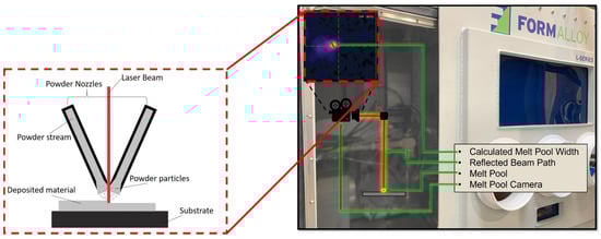
Figure 1.
Schematic of FormAlloy L2 metal AM system with MPS Camera.
Each cylinder has the following features: (1) 1.2 mm wall thickness, (2) 51 mm height, and (3) 13 mm diameter (Figure 2). To generate the tool path a CAD model was imported into a DED tool path generation software and certain parameters (such as laser power, feedrate, and slice/layer thickness) were set. As a baseline, laser power and feedrate were set at the FormAlloy developed values of 225 W and 1000 mm/min, respectively. Each layer thickness was set the same for both samples and a total of 284 layers (0.18 mm individual layer thickness) were generated to manufacture the samples. The software then generates a G-code file which can be uploaded on the FormAlloy L2. The Inconel 625 powder was sourced from Praxair Surface Technologies (product Ni-328-17) with a particle size distribution between 45 and 106 microns [81]. The parts were printed on a steel substrate with a thickness of 6.35 mm. One sample was built in an open loop where the operator was manually adjusting LP, feed rates (scan speeds), and powder disc speed (controls the powder mass flow rate), to complete the build. An MPS sensor was used in this build to record the width of the melt pool during the build process. The waviness found in open loop sample can be attributed to uneven part temperatures as the sample was being built. For the second sample, the MPS sensor was enabled in closed loop mode, which will adjust the LP based on a targeted MPS. This build was able to be completed with minimal user interaction and higher quality.
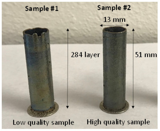
Figure 2.
Inconel 625 sample hollow cylinders.
2.2. Data Collection and Pre-Processing
The following section details the data collection and evaluation process. Figure 3 is a design diagram that describes how the different datasets were organized in the experiment and organizes the process into 4 blocks with 3 phases (data collection, preparation, and analysis). The first block (top left) in Figure 3 refers to how the process parameter dataset was collected in real-time. All process parameters (MPS, Laser Power, etc.) were collected during an actual print and recorded for each layer of the print. After the part was completed, a dataset was created from ex-situ computerized tomography (CT) scans to determine low-density occurrences (based on a threshold) at each layer. The ex-situ process is highlighted in Figure 3 (second block bottom left) and was used to create binary labels of “acceptable” (0) or “unacceptable” (1) layers based on an adjustable threshold and were appended to the process parameter dataset. The focal spot size of the CT scanner is 13.92 microns and it can make enough resolution to discern critical porosities in each layer. Once the dataset was pre-processed and prepared inter-layer feature importance and correlation analysis was conducted, as shown in the third block of Figure 3. Finally, inter-layer feature analysis was performed through the use of an advanced DL technique shown in the fourth block of Figure 3. Additional ML classification techniques were used to classify inter-layer quality of the build using features only and compared to the CNN model in Section 3.
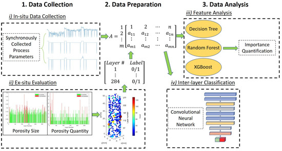
Figure 3.
Design Diagram.
Once both samples were printed, the data generated from the process that features the process parameters and the sensor signatures were used in a post-process analysis. In parallel, the samples were removed from the plate with a wire EDM step and sent to undergo an XCT scan to detect porosity and the location of identified pores.
XCT is defined as a method of establishing 3D representations of objects through obtaining X-ray images centered around an axis of rotation and developing 3D models through algorithms [49,50,51]. Between 2010–2014, XCT became a well-established method for measuring porosity by comparing empty voxels [52]. It has since developed into a nondestructive measuring technique [53,54,55,56].
Table 1 lists all the AM parameters collected synchronously during the AM process of these samples.

Table 1.
AM Parameters.
During the builds of the two samples, around 15–23 data points were collected at each layer (for layers in the uniform portion of the cylinders). The sampling rate was around 0.125 s (8 Hz). In the initial stage, we removed the AM parameter data that (1) is statistically insignificant, and (2) physically may not affect the quality of the part. This resulted in two separate datasets, one containing process parameters during the AM build process and another containing the CT scan features for each of the parts. The raw AM dataset was loaded using the Python pandas package [82] and resulted in a data array of 31 predictors and one response (binary labels of 0 or 1). All 284 layers are utilized in the dataset with each layer containing multiple data points (4950 data points in total for each feature), resulting in a data array of size 31 × 4950 for sample 1 and 2. Labels were created from the CT scan dataset and an adjustable threshold, discussed in Section 2.3. The CT scan dataset contains 33 columns of features and 453 data points for each feature, resulting in a data array of size 31 × 453 for sample 1 and 2. A program was developed to visualize these parameters along with sensed features and data. Figure 4 and Figure 5 isolate the eight synchronously collected parameters during the inter-layer build process of sample #2.
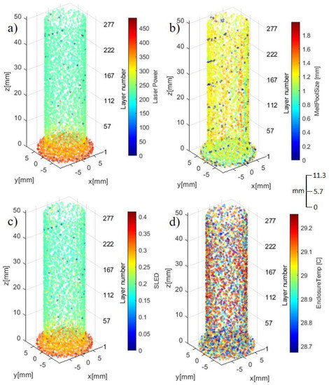
Figure 4.
Synchronously collected process parameters: (a) LP, (b) MPS, (c) SLED, and (d) ET.
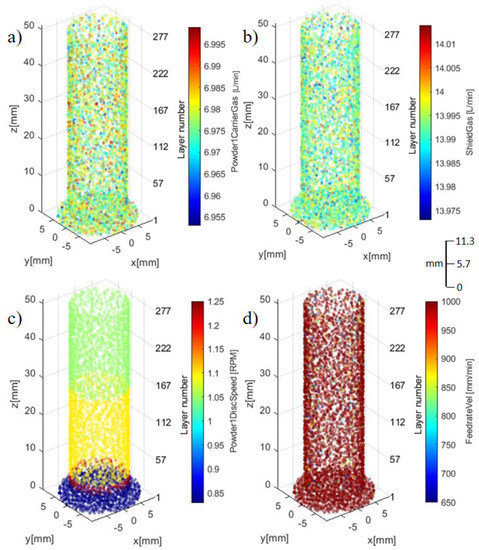
Figure 5.
Synchronously collected process parameters: (a) PCG, (b) SG, (c) PDS, and (d) FR.
In Figure 6, we display the porosity quantities and sizes at the inter-layer level during the build process of workpiece #2 from the CT scan dataset. We can see most of the larger porosities are located between layers 10 to 160.
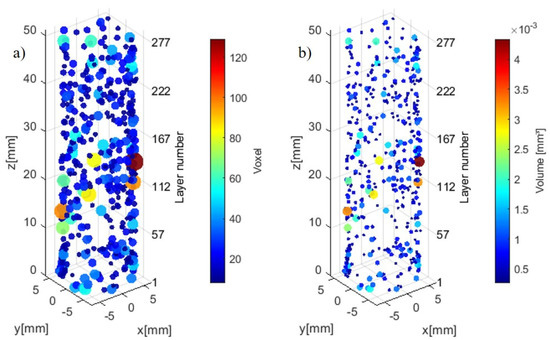
Figure 6.
(a) Inter-layer low-density identification (voxel scale 0.03228 mm) and (b) Volumetric measurement.
2.3. Criteria for Layer Classification
Two criteria were proposed for classifying layers into acceptable or unacceptable classes. The first criterion is based on the maximum diameter of the detected low-density indications, such as porosities. The second criterion was based on the quantity of low-density areas, such as porosities within each layer. The criteria are adjustable to fit different applications based on the required standard. For our investigation, we determined that layers with either low-density indication diameters larger than 0.2 mm or if the number of times a low-density occurrence is identified in a layer exceeds 5, that layer is identified as unacceptable. Figure 7a,b reflect the threshold and ultimately the label feature associated with our classification model. In the bar chart, layers colored in red were deemed unacceptable and green layers were deemed acceptable. As labels, unacceptable layers were appended as 1 and acceptable layers appended as 0.

Figure 7.
Porosity inter-layer evaluation (a) porosity diameter (mm) and (b) porosity quantity.
2.4. Feature Importance and Selection
To our knowledge, the importance of features in a layer-by-layer classification method have not been quantified yet. The synchronous data collection method that we employ for collecting process parameters in real-time allows for the possibility of exploring inter-layer feature relationships. Therefore, we have tested several methods for importance quantification including (1) Decision Tree (DT), (2) Random Forest (RF), and (3) XGBoost (XGB) and compare these results. We value the RF ensemble method for feature importance quantification and use RF for baseline classification comparison to the CNN model. For the RF model, we use feature selection to reduce the feature dataset when predicting only with the RF technique. Feature selection was not utilized for the SVM or CNN models. The five most important features are used as the only variables input into our RF classification experiment. Results are reviewed in Section 3. However, the main focus of our feature analysis is to determine which features are most important for classification and to explore relationships among features at the inter-layer level. These results are displayed in Section 3.1.
Literature defines feature selection as the development of reducing a subset of an originally complete feature dataset using a feature selection process [83]. Whenever a dataset is deemed highly dimensional or dynamical (or both), it is advantageous for the experimenter to reduce the workable dataset, especially when features are highly correlated. By performing feature selection, the overall experiment reduces computation time, improves prediction performance, and allows for more comprehension of results in a ML or pattern recognition investigation [84].
Inter-Layer Importance Quantification
Classification and Regression Trees (CART), also known as Decision Trees (DT), ML techniques utilized for creating prediction models from data [85]. The Gini index is a measure of impurity between the probability distribution and the target attributes values [86]. In the case of classification DT models, it is common to utilize the gini index cost function especially in situations where the domain of the target attribute is not wide [86]. Gini index for a given node in a binary classification problem is defined as [87]:
Here, and represent Class 1 and Class 2. When the Gini index is calculated it reports a Gini score to determine splits based on the purity of the classes. As an example, a perfect separation of classes will result in a Gini score of 0. After the Gini score evaluates the cost of the split, each value within the dataset is evaluated as a candidate for splitting. Once the algorithm finds the best split a node is created, the first node created is typically called the root node. The tree is grown by repeating this process. The user can establish how large the tree will grow based on stopping rules.
The Random Forest (RF) technique is an ensemble method with advantageous capabilities compared to other ML techniques due to its robustness, accuracy, and easily interpretable results in the form of ranking [88]. RF was introduced by Breiman in [89] and is used for reducing variance and utilizes bootstrap aggregation (bagging) to comprise a mean about noisy and unbiased models [90]. The process begins by connecting multiple decision trees in which random selection of input variables bootstraps on a dataset. This forms a forest of classifiers that vote for a particular class and de-correlates the ensemble of decision trees without increasing the variance [91]. Another feature of this method is that RF introduces randomness to the tree-growing process. RF selects m variables by randomly pulling from p variables so that . Once a tree model is trained random splits are generated and selected from the original predictors. The predictor with the best potential is selected and the data is partitioned from that predictor. Then, standard tree rule stopping is employed and pruning is not performed. The driving force behind this process is the predictor, mathematically represented as [91] (for classification and regression, respectively):
where B is the total number of trees that we are predicting on a new point x. An essential aspect of this project was to identify the most influential features during a build process that have the highest impact on part defects. It was necessary to determine which features based on individual layer parameters are most useful for accurate predictions of acceptable and unacceptable layers.
Extreme gradient boost (XGBoost) is a tree boosting ML system that is largely scalable and used for applications like data-driven prediction [92]. Chen and Guestrin, the inventors of XGBoost, ”proposed a sparsity aware algorithm for handling sparse data and a theoretically justified weighted quantile sketch for approximate learning” [92]. The algorithm is a highly scalable end-to-end tree boosting system. The weighted quantile sketch works by approximating candidate split points as a rank:
where, is the rank function, is a multi-set dataset with x predictors, are weights, k is a feature value, and, ∈ is an approximation factor. Chen and Guestrin state that ”most existing approximate algorithms either resorted to sorting on a random subset of data which have a chance of failure or heuristics that do not have a theoretical guarantee”. To address this issue they introduce ”a novel distributed weighted quantile sketch algorithm that can handle weighted data”. Using the exact greedy algorithm is computationally expensive to create splits upon continuous features. An approximate algorithm is used to split upon features based on percentiles of feature distribution. From there, maps are created to place continuous features into buckets split by the established candidates. The best solution is determined based on proposals of aggregated statistics.
The advantage of using these three feature analysis algorithms is that scores can be reported as importance values. In Section 3.1, a thorough comparison of the techniques is discussed.
2.5. DL Networks
Traditional ML tasks are used for a variety of applications but were limited in the past based on their capacity to process natural data in raw form [66]. For this reason a method was needed to automatically handle natural data in raw form. DL techniques thrive at this due to the ability of the algorithms to utilize a general-purpose learning procedure and allow the algorithm to create layers of features instead of humans [66]. We have set this experiment up in a supervised learning fashion. This implies that we supplied each observation with a label [68]. The following section describes the details of the methodology of how we constructed, trained, and tested our DL technique.
2.5.1. Networks and Performance Metrics
Convolutional Neural Networks (CNN) introduced in [93] and popularized in [94], are a specific type of NN used for processing data that has a known grid-like topology [68]. These networks have also been utilized for time-series classification in conjunction with Convolutional Neural Networks (CNN) [95]. When applying a supervised algorithm the typical aim is to optimize the weights and biases and ultimately reduce the error between predicted () and actual (y) values. Binary cross-entropy (BCE) loss has been utilized across many ML applications for assessing the difference between a predicted label and a true label of CNN models for classification [96,97,98]. This experiment aims to minimize error, ergo the cost (sometimes called loss) function utilized to optimize error of the CNN is [96]:
where, T is the true label, is an individual element of that label, and P is the prediction of the output and is a single element of that particular prediction.
The confusion matrix is defined in Table 2:
Table 2.
Confusion Matrix.
Where represents the i actual observations and j predictions. True Positive (TP) occurs when the sample is positive and predicted to be positive. True Negative (TN) takes place when a negative case occurs and is predicted to be negative. An occurrence of False Positive (FP) errors happens with an actual negative case predicted positive (Type I error) and False Negative (FN) error occurs when an actual case is positive and prediction is negative (Type II error). Some situations may prepare for Type I and Type II errors differently. Prediction models can be ‘adjusted’ to reduce Type II errors which in turn could allow for more Type I errors and vice versa. In our case there is not a detrimental effect of either of these errors, so we do not penalize our prediction model to account for the errors.
We define performance metrics from the binary confusion matrix as [99]:
2.5.2. Classification Network Structure
First, we train a DL network that does not consider time dependency and therefore order of arrival of each data point is not a concern. The focus of this network is to determine if patterns can be recognized in the data features and provide a comparison to the CNN model. Figure 8 displays the CNN architecture used for classification process of layer-wise dataset.
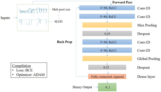
Figure 8.
CNN architecture.
A typical CNN structure is constructed with a convolutional layer which contains filters (F) and activation functions (g) [99]. The activation function used for both convolutional layer stacks is the ReLU function from Equation (1). In our network, we stack two convolutional layers which then feed to a pooling layer. By stacking the two convolutional layers we theoretically create a hierarchical decomposition of the raw input data [100,101,102,103]. Output from the convolution stack is fed to a max pooling layer. Max pooling is used in our network mainly due to better performance when compared to average pooling [104]. This layer reduces the spatial size by extracting feature maps through means of downsampling (reduction of parameters). Since we have a single model, research suggests the proper method to reduce over-fitting in single, fixed-size models is by applying the dropout technique [105]. Therefore, the feature map is then applied to dropout set to 0.25, meaning 25% of the inputs are dropped. This process is repeated (and can be repeated as many times as specified) upon which the feature map reaches the fully connected (dense) layer and is flattened (transformed into 1D). During this layer a multi-layer perceptron (MLP) is fit on the feature map.
Raw data from sample 1 and 2 were imported to the classification model in the comma-separated value (.csv) format. Then, each dataset is cleaned and prepared with the removal of rows lacking values or containing empty cells (NaN) and unnecessary columns. Once the cleaning was complete, the data was normalized between a range of (0, 1). Next, the data was reshaped and prepared for training on a 75/25 split (training/testing, respectively). Using Keras [106] and TensorFlow [107] packages in Python, the model is formatted to a sequential model with Conv1D layers which creates a convolution kernel that is convolved with the input through a single spatial dimension to create tensors of outputs. All experiments were run on an Intel(R) Core(TM) i7-10700 CPU @ 2.90GHz, 2.90 GHz with 64.0 GB of RAM. The raw data, after cleaning, has 4950 rows and 11 features . Raw data was reshaped into a 3D tensor with the shape of (time steps, features, sample). A reshape function from the numpy library [108] is executed that accepts a tuple argument and we train one sample at a time so the data now takes the form: . Experiments are run through 100 epochs with a batch size of 16 for both samples, testing is performed on each sample. During training, the model slices the inputs into batch sizes then iterates over a user specified number of epoch cycles. The model iterates over the validation dataset computing the validation loss at the end of each epoch. Using Equation (8), the error is calculated at the end of each epoch. We use the sigmoid activation function to perform binary classification on the output vector. During back-propagation we utilize the standard gradient decent algorithm optimized by Adaptive Moment Estimation (ADAM) [109].
3. Results and Discussion
In this study, the use of a specific material and geometry does limit the generalizability of the results obtained. Presented here are specific results that lend credence to the methodology developed. Generalizability, if it is a realistic proposition, will come from a continued study including multiple geometries and materials all under this data-driven paradigm. The following section evaluates these results obtained during experimentation.
3.1. Tree-Based Feature Importance
Using RF technique, we produced feature importance charts. During this method, importance measures determine the split when growing a decision tree. Figure 9 depicts the relative variable importance of the most influential features for predicting good layers in the DED process for (a) A Single Decision Tree, (b) An Ensemble of Decision Trees, and (c) XGBoost technique. Intuitively comparing DT and RF importance values suggests that the values measured from RF are more reliable. Therefore, we select features from RF to feed into our CNN model. The barchart from XGBoost technique is slightly more nontransparent since there is a clear bias towards contour flag and other features are not considered important.
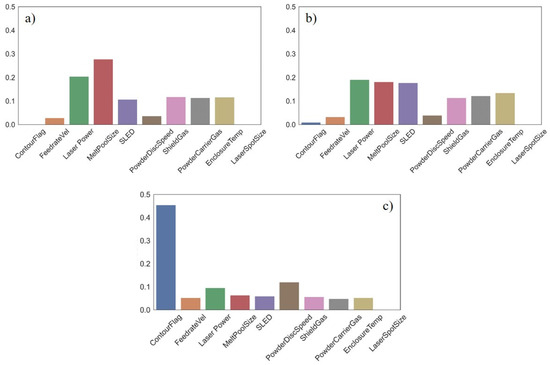
Figure 9.
Feature importance bar plots: (a) Decision Tree, (b) Random Forest, (c) XGBoost.
Importance values calculated from RF technique show that the five most influential features are, (1) LP (0.19), (2) MPS (0.18), (3) SLED (0.18), (4) ET (0.13), and (5) PCG (0.12). Figure 10 demonstrates the features upon which the RF selected for splits. During this ensemble we restricted the RF to 3 levels as to not overgrow our model and lose interpretability. The main root begins by splitting upon the LP feature which splits at a value of 362.5 W. From there, two branches are created. Samples less than or equal to 362.5 W split to the left branch and samples with higher LP values split to the right. The left branch splits upon LP again at a value of 286.2 W. Samples with values less than 286.2 W move to a branch (left) dictated by the PDS which splits at a value of 1.1 RPM, while samples with a value greater than or equal to 286.2 W filter to another branch dictated by LP at a value of 289.5 W. Both of these branches lead to leaf nodes. Moving back to the root node, if a sample has an LP value more than 362.5 W it splits to the right branch. This branch is decided by MPS at a value of 1.3 mm. Samples with MPS less than or equal to 1.3 mm are organized to another branch predicated on PDS and move to a leaf node depending on corresponding PDS values. If a sample possesses MPS greater than 1.3 mm they are split to a branch based on SLED. These samples then are split into leaf nodes. Most samples (1180 + 1120) are filtered down the path that splits upon LP 362.5 W → LP 286.2 W→ PDS. Samples following that path are all deemed good. When we evaluate XGBoost and the bias it has towards contour flag further with the heat map in Figure 11, we can see a possible explanation. There are several features highly correlated with the contour flag feature. These same features (LP, MPS, and SLED) are measured as highly important from the RF algorithm.

Figure 10.
RF tree.

Figure 11.
Heat map comparison of all features.
Table 3 showcases the measures of importance from each of the three feature selection techniques. We understand that the RF technique provides more confidence in the splits compared to the decision tree method since RF is an ensemble of trees. Thus, for this reason we do not consider the measures from the decision tree for feature reduction. The XGBoost technique was eliminated from consideration due to poor results. In the XGBoost, the model predicts that most of the importance comes from the CF feature (0.44). The remaining features carry little to no weight which is not useful for this investigation.
Table 3.
Comparison of feature selection techniques.
Figure 11 shows the correlation amongst the 8 most correlated features in the experiment. The features with the most correlation are SLED and LP with a positive relationship of 0.97. This relationship demonstrates almost a direct linear and positive trend between the two features which is expected since SLED is calculated with input from LP. CF has relationships with PDS (0.79), LP (−0.67), SLED (−0.65), MPS (0.39), and feed rate (−0.13). Negative correlations exist between LP/PDS (−0.66), LP/CF (−0.67), SLED/PDS (−0.66), and SLED/CF (−0.65). From this data we can safely determine that the CF has relationships with the majority of the features that are responsible for prediction performance. Of those features, LP, MPS, and SLED are the most important features for affecting prediction of the classification model. CF has a strong correlation to these three features.
Feature Analysis
In Figure 4, Figure 5 and Figure 6 a visual analysis of the parameters is observed during a build process, while this information is important during in situ monitoring, a statistical/qualitative analysis is very important to evaluate the parameters of the build process. Therefore, in the following section an in-depth analysis explores parameters collected from sample 2 while it was built.
Considering the 5 most impactful features during the build process, this section is dedicated to analyzing and visualizing the most important features through the building of sample 2. Figure 12 displays the LP, MPS, and SLED features throughout the build process for sample 2. The base of sample 2 consists of the first 6 layers, this is noticeable in the dataset. Layers 1 through 6 consist of at least 155 to 174 data points while layers 7 through 284 all contain under 20 data points. Through this logic, we define the base as layers 1 through 6 and the shaft as layers 7 through 284. The base of all three visualizations in Figure 12, circled in red, demonstrates a distinct grouping of measurements when compared to the shaft portion of the sample.
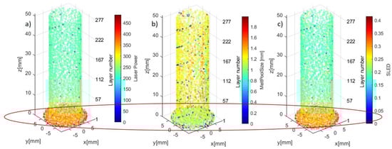
Figure 12.
Visualization of features of build of (a) LP, (b) MPS, and (c) SLED.
Table 4 showcases a value comparison of the 5 most impactful features for classification between the base and shaft. This table demonstrates that the base experiences a significantly higher LP usage and smaller overall MPS. Variations in LP, MPS, and SLED are higher when building the base and have less deviation through the building of the shaft. The largest MPS occurs when building the shaft with a value of 1.989 mm. The small amount of variation in the features when building the shaft may be responsible for over-fitting of the CNN model. Evaluation of this topic is explored deeper in Section 3.2.1.
Table 4.
Comparison of feature throughout build.
Table 5 separates the features based on labels in an effort to describe the values of the features based on layer quality. Average wattage and variance for LP are higher in layers deemed acceptable. The highest recorded LP measure occurs within an unacceptable layer. The sizes of melt pools on average are smaller (0.033 mm) for acceptable layers however, the largest MPS occurs within an acceptable layer.
Table 5.
Comparison of features based on layer quality.
3.2. CNN
The data is preprocessed and standardized (normalizing values 0 to 1) prior to training. This feature scaling technique is the process of casting data of predictors into a specific range values [110]. Feature scaling is a vital component for the success of ML algorithms because it prevents large numeric feature values from overshadowing smaller numeric features values [111]. We use a wrapper, KerasClassifier framework which is a common tactic for baseline classification results [112,113], and use the model to classify layers as acceptable and unacceptable. The Keras DL model classifies with an accuracy of 84.89%. Using the top five most influential features, we created a classification model using RF to determine if any improvement is made to classification. Completion of the RF model with these features rendered an overall classification accuracy of 89%. The SVM We use these results as a baseline to compare and improve upon with the CNN model. Inputs for all classification models are the standardized and synchronously collected process parameters. All outputs for classification models are either 0 representing acceptable layers or 1 representing unacceptable layers. These results are used as a baseline to compare and potentially improve upon with the CNN model. In total, we trained SVM with four kernels, RF classifier, and Keras classifier and compared results to the CNN model. Table 6 displays the highest recorded accuracy measurements of these methods. The CNN classifies at the same rate as the SVM with linear, poly, and rbf kernals.
Table 6.
Accuracy comparison.
3.2.1. Evaluation of Over-Fitting
While it is advantageous to have a classification model equipped with the ability to perform high-level classifications with raw AM process parameter inputs, the current form of the algorithm is not without limitations. DL algorithms become highly effective at prediction and classification as datasets become larger. When the training data is smaller, DL algorithms can result in issues of overfitting. This occurred during the training process of both samples.
In Figure 13a,b, we showcase how the CNN trains through a total of 100 epochs. Seen in Figure 13, training accuracy trends in an increasing fashion with some fluctuation throughout the process. The validation measure is seen to converge on training around the 62nd epoch. Upon that, training and validation results appear to diverge as epochs increase. Looking at Figure 13b the overall loss plot is displayed throughout the training process. It can be seen around the 62nd epoch that validation loss crosses the training loss threshold which corresponds with the ‘shuttlewise’ movement in validation accuracy after the 62nd epoch from the accuracy plot. Every additional epoch shows that the validation loss increases which indicates over-fitting is occurring during training. This issue is evaluated further in Section 3.2.1.
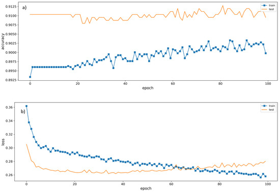
Figure 13.
CNN training plots of (a) accuracy and (b) loss.
The results from Section 3.2 in conjunction with the training plots indicate that the CNN trained and tested on data from sample 2 experienced over-fitting even when building the model using the dropout technique. The remainder of this subsection explores the results gathered while training and testing on both sample 2 (acceptable sample) and sample 1 (unacceptable sample). Over-fitting occurs in DL when the model becomes oversaturated (or over-dependent) from the training dataset and learn incorrect mapping [114,115]. To fix this issue, some research has focused on L2 regularization. In [115], an adjustment to the Loss (or Cost) Function is made as:
where is the modified Loss function, L is the Loss (or Cost) function from the DL model. is a hyperparameter that adjusts the strength of the regularization and is the updating parameter in the stochastic gradient descent (SGD) optimization equation, while there are many methods to solve the case of over-fitting, this study is focused on reporting results of CNN classification at the inter-layer level and comparing these results with other ML techniques.
Figure 14a,b show the acceptable and unacceptable layers throughout each layer during the build process of sample 1. Figure 14a shows layer classification based on the size of low-density occurrences and Figure 14b shows the quantity of low-density occurrences for each layer of sample 1. It can be seen in these two figures that the majority of unacceptable layers are located early in the build process. Most unacceptable low-density occurrences occur between layers 50 and 125.
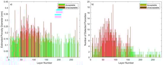
Figure 14.
Porosity inter-layer evaluation: (a) low-density diameter of Sample 1 (mm) and (b) low-density quantity of sample 1.
Figure 15 confirms that the majority of low-density occurrences occur earlier in the build process for sample 1. This is quite different from sample 2, shown in Figure 6, where the low-density occurrences happen more uniformly throughout the build process.
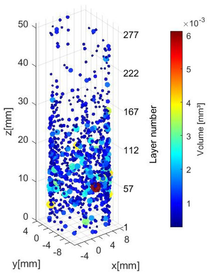
Figure 15.
Inter-layer low-density identification of sample 1 (voxel scale 0.03228 mm).
Table 7 summarizes an in-depth analysis of the performance of both samples. We show the capabilities of the CNN model and determine that features can be utilized for accurate layer-wise classification with an average accuracy of 75.9% when trained on a low-quality sample and 78.4% when trained on a high-quality sample. Specificity measurements indicate that the proportion of actual negative cases was predicted correctly on average 65.9% of the time when trained on sample 1 and 12% on average when trained on sample 2. However, sensitivity measures, which are the proportion of actual positive cases predicted correctly, was measured on average to be 78.2% and 95.5% when trained on a low and high-quality sample, respectively. We point out that the sensitivity metric is more impactful here since it is responsible for the majority of cases (shown in detail in Figure 16a,b)). The results of the sensitivity/specificity indicate that the CNN model is very sensitive and effective at determining bad layers as bad which means few cases of bad layers are misidentified. The low specificity suggests that the model does identify some good layers as bad layers. This is important in this investigation since layers with defects can render a sample defective. Table 7 showcases how the accuracy of the CNN drops significantly from 88.8% to 68.1% when trained on a high-quality sample and tested on a low-quality sample, a 23% drop. Sample 1 demonstrates a 25% drop in accuracy when tested on sample 2.
Table 7.
CNN performance on all samples.
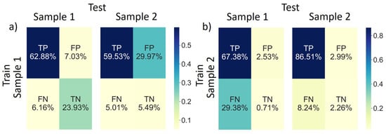
Figure 16.
Confusion matrix training on (a) sample 1 and (b) sample 2.
The highly informative F1 scores are reported in Table 8. It is demonstrated that when we train this CNN on a high-quality sample, the model performance peaks with F1 scores of 80.9% and 93.98% when tested on a low-quality sample and high-quality sample, respectively.
Table 8.
F1 Scores.
The confusion matrices from Table 2 are shown in Figure 16a,b for training on sample 1 and 2, respectively. The majority of cases are True Positive indicating that the CNN identifies actual positive cases the most. When training and testing on the same sample, TP is the highest which was expected. When trained on the low-quality sample and tested on the high-quality sample, False Positives are the highest of all combinations. This information is important, indicating that when trained on a low-quality sample and testing on a high-quality sample a higher rate of falsely identifying positive cases occurs. This is not the case when trained on a high-quality sample. Figure 16b highlights FP percentages of 2.53 and 2.99 when tested on low-quality and high-quality samples, respectively.
4. Conclusions
In this study, we present a nondestructive synchronous method that monitors quality of a workpiece during a metal AM build process. The investigation innovates based on two main concepts. The first concept is that we use a synchronously collected in situ dataset with low sampling rate in conjunction with an ex-situ evaluation based on CT scans of parts to create a labeling dataset. The second concept is the application of a CNN algorithm that classifies inter-layer quality through the build process of a part based on in situ input data and ex-situ labels. This method resulted in a dataset of process parameters collected during in situ quality monitoring. The printed workpiece was analyzed for low-density occurrences via a CT scan. An adjustable threshold was created to qualify specific layers as acceptable or unacceptable. Using a combination of the synchronous process parameter dataset and layer qualification dataset, we investigate the importance of specific features during real-time LB-DED printing at the inter-layer level. We show that LP, MPS, and SLED have the most impact on prediction, with CF having a strong correlation to those three features. We explore the relationships between features to establish that certain features are correlated with each other while the workpiece is being produced. In this investigation, we demonstrate that even though the use of a specific material and geometry does limit the generalizability of the results obtained, possibly leading to over-fitting, a DL classification model is capable of classifying acceptable and unacceptable layers and could be implemented into an in situ quality monitoring setting through training of features during a build process at the interlayer level. We use the layer qualification dataset to establish a set of labels that are used for training with the synchronous process parameter dataset as inputs. Compared to similar in situ quality monitoring AM studies, we do not utilize acoustic emission or other NDT data with high sampling rates (e.g., MHz) for classification and show the possibility of using a dataset with a low sampling rate (e.g., Hz) for simple and reduced data size training in the classification models. Results indicate over-fitting occurs when training and testing on a sample of a similar shape. Further analysis confirms over-fitting from the CNN when training and testing on separate samples, however, the CNN model is promising for in situ layer classification. The AM process has limited features which could be one reason why the classification model is overfitting. The addition of other NDT methods may remove statistical bias and may improve the information mapping process of the algorithm. For example, adding acoustic emission data in parallel to recording the printing parameters would allow for deeper and more accurate monitoring as the AM machine builds parts. We are confident that adding such a dataset to the classification model would increase the robustness of the training and testing process and reduce statistical bias of the algorithm.
Author Contributions
Conceptualization, E.D.-N., K.L. and H.S.H.; methodology, M.J., K.L. and H.S.H.; software, S.H.; formal analysis, S.H.; investigation, S.H., M.J., H.S.H. and E.D.-N.; resources, E.D.-N., M.J., K.L. and H.S.H.; writing—original draft preparation, S.H.; writing—review and editing, S.H., M.J. and E.D.-N.; visualization, S.H., E.D.-N.; supervision, E.D.-N.; project administration, E.D.-N.; funding acquisition, E.D.-N. All authors have read and agreed to the published version of the manuscript.
Funding
This material is based upon work supported by the National Aeronautics and Space Administration (NASA) under Grant No. 80NSSC20C0303 issued through the Small Business Technology Transfer (STTR) program. We are also gratefully acknowledge the funding support from Department of Energy/National Nuclear Security Agency (Grant DE-NA0003987) and National Science Foundation (NSF) (Grant 1840138).
Institutional Review Board Statement
Not applicable.
Informed Consent Statement
Not applicable.
Data Availability Statement
The datasets generated during and/or analysed during the current study are not publicly available due to a nondisclosure agreement as part of collaborative NASA STTR Phase I project between FormAlloy Company and New Mexico State University but are available from the corresponding author on reasonable request.
Acknowledgments
The authors would like to express their sincere gratitude to FormAlloy Company in particular Jeff Riemann and Melanie Lang for their support.
Conflicts of Interest
The authors declare no conflict of interest.
References
- Noorani, R. Rapid Prototyping: Principles and Applications; John Wiley & Sons Incorporated: Hoboken, NJ, USA, 2006. [Google Scholar]
- Gibson, I.; Rosen, D.; Stucker, B.; Khorasani, M. Additive Manufacturing Technologies; Springer: Cham, Switzerland, 2014; Volume 17. [Google Scholar]
- Kumar, M.B.; Sathiya, P. Methods and materials for additive manufacturing: A critical review on advancements and challenges. Thin-Walled Struct. 2021, 159, 107228. [Google Scholar] [CrossRef]
- Durakovic, B. Design for additive manufacturing: Benefits, trends and challenges. Period. Eng. Nat. Sci. PEN 2018, 6, 179–191. [Google Scholar] [CrossRef]
- Khorasani, M.; Ghasemi, A.; Rolfe, B.; Gibson, I. Additive manufacturing a powerful tool for the aerospace industry. Rapid Prototyp. J. 2021, 28, 87–100. [Google Scholar] [CrossRef]
- Hung, C.H.; Turk, T.; Sehhat, M.H.; Leu, M.C. Development and experimental study of an automated laser-foil-printing additive manufacturing system. Rapid Prototyp. J. 2022, 28, 1013–1022. [Google Scholar] [CrossRef]
- Riensche, A.; Severson, J.; Yavari, R.; Piercy, N.L.; Cole, K.D.; Rao, P. Thermal modeling of directed energy deposition additive manufacturing using graph theory. Rapid Prototyp. J. 2022. ahead-of-print. [Google Scholar] [CrossRef]
- Panchagnula, J.S.; Simhambhatla, S. A novel methodology to manufacture complex metallic sudden overhangs in weld-deposition based additive manufacturing. Rapid Prototyp. J. 2022. ahead-of-print. [Google Scholar] [CrossRef]
- Gunasekaran, A.; Subramanian, N.; Ngai, W.T.E. Quality Management in the 21st Century Enterprises: Research Pathway towards Industry 4.0. Int. J. Prod. Econ. 2019, 207, 125–129. [Google Scholar] [CrossRef]
- Hsu, T.C.; Tsai, Y.H.; Chang, D.M. The Vision-Based Data Reader in IoT System for Smart Factory. Appl. Sci. 2022, 12, 6586. [Google Scholar] [CrossRef]
- Tofail, S.A.; Koumoulos, E.P.; Bandyopadhyay, A.; Bose, S.; O’Donoghue, L.; Charitidis, C. Additive manufacturing: Scientific and technological challenges, market uptake and opportunities. Mater. Today 2018, 21, 22–37. [Google Scholar] [CrossRef]
- Dehghan Niri, E.; Kottilingam, S.C. Method and System for In-Process Monitoring and Quality Control of Additive Manufactured Parts. U.S. Patent App. 15/290,078, 12 April 2018. [Google Scholar]
- Dehghan Niri, E.; Lochner, C.J.; Luo, K. Method and System for Topographical Based Inspection and Process Control for Additive Manufactured Parts. U.S. Patent App. 15/290,067, 12 April 2018. [Google Scholar]
- DehghanNiri, E.; Kottilingam, S.C.; Going, C.L. Method and System for X-ray Backscatter Inspection of Additive Manufactured Parts. U.S. Patent 10,919,285, 16 February 2021. [Google Scholar]
- Park, H.; Ko, H.; Lee, Y.t.T.; Feng, S.; Witherell, P.; Cho, H. Collaborative knowledge management to identify data analytics opportunities in additive manufacturing. J. Intell. Manuf. 2021, 1–24. [Google Scholar] [CrossRef]
- Kottilingam, S.C.; Going, C.L.; DehghanNiri, E. Method and System for Thermographic Inspection of Additive Manufactured Parts. U.S. Patent App. 15/296,354, 19 April 2018. [Google Scholar]
- DehghanNiri, E.; Rose, C.W.; McCONNELL, E.E. Method and System for Inspection of Additive Manufactured Parts. US Patent App. 15/230,579, 8 February 2018. [Google Scholar]
- Roh, B.M.; Kumara, S.R.; Yang, H.; Simpson, T.W.; Witherell, P.; Lu, Y. In-Situ Observation Selection for Quality Management in Metal Additive Manufacturing. In Proceedings of the International Design Engineering Technical Conferences and Computers and Information in Engineering Conference. American Society of Mechanical Engineers, Virtual, Online, 17–19 August 2021; Volume 85376, p. V002T02A069. [Google Scholar]
- Zhang, Y.; Wu, L.; Guo, X.; Kane, S.; Deng, Y.; Jung, Y.G.; Lee, J.H.; Zhang, J. Additive manufacturing of metallic materials: A review. J. Mater. Eng. Perform. 2018, 27, 1–13. [Google Scholar] [CrossRef]
- Onuike, B.; Heer, B.; Bandyopadhyay, A. Additive manufacturing of Inconel 718—Copper alloy bimetallic structure using laser engineered net shaping (LENS™). Addit. Manuf. 2018, 21, 133–140. [Google Scholar] [CrossRef]
- Kim, G.; Oh, Y. A benchmark study on rapid prototyping processes and machines: Quantitative comparisons of mechanical properties, accuracy, roughness, speed, and material cost. Proc. Inst. Mech. Eng. Part B J. Eng. Manuf. 2008, 222, 201–215. [Google Scholar] [CrossRef]
- Tang, Z.J.; Liu, W.W.; Wang, Y.W.; Saleheen, K.M.; Liu, Z.C.; Peng, S.T.; Zhang, Z.; Zhang, H.C. A review on in situ monitoring technology for directed energy deposition of metals. Int. J. Adv. Manuf. Technol. 2020, 108, 3437–3463. [Google Scholar] [CrossRef]
- Aminzadeh, M.; Kurfess, T.R. Online quality inspection using Bayesian classification in powder-bed additive manufacturing from high-resolution visual camera images. J. Intell. Manuf. 2019, 30, 2505–2523. [Google Scholar] [CrossRef]
- Kwon, O.; Kim, H.G.; Ham, M.J.; Kim, W.; Kim, G.H.; Cho, J.H.; Kim, N.I.; Kim, K. A deep neural network for classification of melt-pool images in metal additive manufacturing. J. Intell. Manuf. 2020, 31, 375–386. [Google Scholar] [CrossRef]
- Charalampous, P.; Kostavelis, I.; Tzovaras, D. Non-destructive quality control methods in additive manufacturing: A survey. Rapid Prototyp. J. 2020, 26, 777–790. [Google Scholar] [CrossRef]
- Masinelli, G.; Shevchik, S.A.; Pandiyan, V.; Quang-Le, T.; Wasmer, K. Artificial Intelligence for Monitoring and Control of Metal Additive Manufacturing. In Proceedings of the International Conference on Additive Manufacturing in Products and Applications; Springer: Zurich, Switzerland, 2020; pp. 205–220. [Google Scholar]
- Tian, Q.; Guo, S.; Melder, E.; Bian, L.; Guo, W. Deep learning-based data fusion method for in situ porosity detection in laser-based additive manufacturing. J. Manuf. Sci. Eng. 2021, 143, MANU-20-1337. [Google Scholar] [CrossRef]
- Shevchik, S.A.; Masinelli, G.; Kenel, C.; Leinenbach, C.; Wasmer, K. Deep learning for in situ and real-time quality monitoring in additive manufacturing using acoustic emission. IEEE Trans. Ind. Inform. 2019, 15, 5194–5203. [Google Scholar] [CrossRef]
- Sanaei, N.; Fatemi, A. Defects in additive manufactured metals and their effect on fatigue performance: A state-of-the-art review. Prog. Mater. Sci. 2020, 117, 100724. [Google Scholar] [CrossRef]
- Anderegg, D.A.; Bryant, H.A.; Ruffin, D.C.; Skrip, S.M., Jr.; Fallon, J.J.; Gilmer, E.L.; Bortner, M.J. In-situ monitoring of polymer flow temperature and pressure in extrusion based additive manufacturing. Addit. Manuf. 2019, 26, 76–83. [Google Scholar] [CrossRef]
- Jafari-Marandi, R.; Khanzadeh, M.; Tian, W.; Smith, B.; Bian, L. From in situ monitoring toward high-throughput process control: Cost-driven decision-making framework for laser-based additive manufacturing. J. Manuf. Syst. 2019, 51, 29–41. [Google Scholar] [CrossRef]
- Everton, S.K.; Hirsch, M.; Stravroulakis, P.; Leach, R.K.; Clare, A.T. Review of in situ process monitoring and in situ metrology for metal additive manufacturing. Mater. Des. 2016, 95, 431–445. [Google Scholar] [CrossRef]
- Shevchik, S.A.; Kenel, C.; Leinenbach, C.; Wasmer, K. Acoustic emission for in situ quality monitoring in additive manufacturing using spectral convolutional neural networks. Addit. Manuf. 2018, 21, 598–604. [Google Scholar] [CrossRef]
- Lewandowski, J.J.; Seifi, M. Metal additive manufacturing: A review of mechanical properties. Annu. Rev. Mater. Res. 2016, 46, 151–186. [Google Scholar] [CrossRef]
- Shirazi, S.F.S.; Gharehkhani, S.; Mehrali, M.; Yarmand, H.; Metselaar, H.S.C.; Kadri, N.A.; Osman, N.A.A. A review on powder-based additive manufacturing for tissue engineering: Selective laser sintering and inkjet 3D printing. Sci. Technol. Adv. Mater. 2015, 16, 033502. [Google Scholar] [CrossRef]
- Taheri, H.; Koester, L.W.; Bigelow, T.A.; Faierson, E.J.; Bond, L.J. In situ additive manufacturing process monitoring with an acoustic technique: Clustering performance evaluation using K-means algorithm. J. Manuf. Sci. Eng. 2019, 141, 041011. [Google Scholar] [CrossRef]
- Nasiri, A.; Bao, J.; Mccleeary, D.; Louis, S.Y.M.; Huang, X.; Hu, J. Online Damage Monitoring of SiC f-SiC m Composite Materials Using Acoustic Emission and Deep Learning. IEEE Access 2019, 7, 140534–140541. [Google Scholar] [CrossRef]
- Wang, S.; Lasn, K.; Elverum, C.W.; Wan, D.; Echtermeyer, A. Novel in situ residual strain measurements in additive manufacturing specimens by using the Optical Backscatter Reflectometry. Addit. Manuf. 2020, 32, 101040. [Google Scholar] [CrossRef]
- Jin, Z.; Zhang, Z.; Gu, G.X. Automated real-time detection and prediction of interlayer imperfections in additive manufacturing processes using artificial intelligence. Adv. Intell. Syst. 2020, 2, 1900130. [Google Scholar] [CrossRef] [Green Version]
- Bappy, M.M.; Liu, C.; Bian, L.; Tian, W. In-situ Layer-wise Certification for Direct Energy Deposition Processes based on Morphological Dynamics Analysis. J. Manuf. Sci. Eng. 2022, 144, 1–35. [Google Scholar] [CrossRef]
- Gobert, C.; Reutzel, E.W.; Petrich, J.; Nassar, A.R.; Phoha, S. Application of supervised machine learning for defect detection during metallic powder bed fusion additive manufacturing using high resolution imaging. Addit. Manuf. 2018, 21, 517–528. [Google Scholar] [CrossRef]
- Abdelrahman, M.; Reutzel, E.W.; Nassar, A.R.; Starr, T.L. Flaw detection in powder bed fusion using optical imaging. Addit. Manuf. 2017, 15, 1–11. [Google Scholar] [CrossRef]
- Davtalab, O.; Kazemian, A.; Yuan, X.; Khoshnevis, B. Automated inspection in robotic additive manufacturing using deep learning for layer deformation detection. J. Intell. Manuf. 2020, 33, 771–784. [Google Scholar] [CrossRef]
- DebRoy, T.; Wei, H.; Zuback, J.; Mukherjee, T.; Elmer, J.; Milewski, J.; Beese, A.M.; Wilson-Heid, A.d.; De, A.; Zhang, W. Additive manufacturing of metallic components–process, structure and properties. Prog. Mater. Sci. 2018, 92, 112–224. [Google Scholar] [CrossRef]
- Paulson, N.H.; Gould, B.; Wolff, S.J.; Stan, M.; Greco, A.C. Correlations between thermal history and keyhole porosity in laser powder bed fusion. Addit. Manuf. 2020, 34, 101213. [Google Scholar] [CrossRef]
- Bauereiß, A.; Scharowsky, T.; Körner, C. Defect generation and propagation mechanism during additive manufacturing by selective beam melting. J. Mater. Process. Technol. 2014, 214, 2522–2528. [Google Scholar] [CrossRef]
- Ronneberg, T.; Davies, C.M.; Hooper, P.A. Revealing relationships between porosity, microstructure and mechanical properties of laser powder bed fusion 316L stainless steel through heat treatment. Mater. Des. 2020, 189, 108481. [Google Scholar] [CrossRef]
- Darvish, K.; Chen, Z.; Pasang, T. Reducing lack of fusion during selective laser melting of CoCrMo alloy: Effect of laser power on geometrical features of tracks. Mater. Des. 2016, 112, 357–366. [Google Scholar] [CrossRef]
- Thompson, A.; Maskery, I.; Leach, R.K. X-ray computed tomography for additive manufacturing: A review. Meas. Sci. Technol. 2016, 27, 072001. [Google Scholar] [CrossRef]
- De Chiffre, L.; Carmignato, S.; Kruth, J.P.; Schmitt, R.; Weckenmann, A. Industrial applications of computed tomography. Cirp Ann. 2014, 63, 655–677. [Google Scholar] [CrossRef]
- Kruth, J.P.; Bartscher, M.; Carmignato, S.; Schmitt, R.; De Chiffre, L.; Weckenmann, A. Computed tomography for dimensional metrology. Cirp Ann. 2011, 60, 821–842. [Google Scholar] [CrossRef]
- Taud, H.; Martinez-Angeles, R.; Parrot, J.; Hernandez-Escobedo, L. Porosity estimation method by X-ray computed tomography. J. Pet. Sci. Eng. 2005, 47, 209–217. [Google Scholar] [CrossRef]
- Siddique, S.; Imran, M.; Rauer, M.; Kaloudis, M.; Wycisk, E.; Emmelmann, C.; Walther, F. Computed tomography for characterization of fatigue performance of selective laser melted parts. Mater. Des. 2015, 83, 661–669. [Google Scholar] [CrossRef]
- Carlton, H.D.; Haboub, A.; Gallegos, G.F.; Parkinson, D.Y.; MacDowell, A.A. Damage evolution and failure mechanisms in additively manufactured stainless steel. Mater. Sci. Eng. A 2016, 651, 406–414. [Google Scholar] [CrossRef]
- Kim, F.H.; Pintar, A.L.; Moylan, S.P.; Garboczi, E.J. The influence of X-ray computed tomography acquisition parameters on image quality and probability of detection of additive manufacturing defects. J. Manuf. Sci. Eng. 2019, 141, 111002. [Google Scholar] [CrossRef] [PubMed]
- Gobert, C.; Kudzal, A.; Sietins, J.; Mock, C.; Sun, J.; McWilliams, B. Porosity segmentation in X-ray computed tomography scans of metal additively manufactured specimens with machine learning. Addit. Manuf. 2020, 36, 101460. [Google Scholar] [CrossRef]
- Matlack, K.H.; Wall, J.; Kim, J.; Qu, J.; Jacobs, L.; Viehrig, H.W. Nonlinear ultrasound to monitor radiation damage in structural steel. In Proceedings of the 6th European Workshop on Structural Health Monitoring, Dresden, Germany, 3–6 July 2012; Volume 1, pp. 138–145. [Google Scholar]
- Honarvar, F.; Varvani-Farahani, A. A review of ultrasonic testing applications in additive manufacturing: Defect evaluation, material characterization, and process control. Ultrasonics 2020, 108, 106227. [Google Scholar] [CrossRef]
- Park, S.H.; Choi, S.; Jhang, K.Y. Porosity Evaluation of Additively Manufactured Components Using Deep Learning-based Ultrasonic Nondestructive Testing. Int. J. Precis. Eng. Manuf. Green Technol. 2021, 9, 395–407. [Google Scholar] [CrossRef]
- Cui, W.; Zhang, Y.; Zhang, X.; Li, L.; Liou, F. Metal additive manufacturing parts inspection using convolutional neural network. Appl. Sci. 2020, 10, 545. [Google Scholar] [CrossRef] [Green Version]
- Sun, W.; Zhang, Z.; Ren, W.; Mazumder, J.; Jin, J.J. In Situ Monitoring of Optical Emission Spectra for Microscopic Pores in Metal Additive Manufacturing. J. Manuf. Sci. Eng. 2022, 144, 011006. [Google Scholar] [CrossRef]
- Zhao, C.; Fezzaa, K.; Cunningham, R.W.; Wen, H.; De Carlo, F.; Chen, L.; Rollett, A.D.; Sun, T. Real-time monitoring of laser powder bed fusion process using high-speed X-ray imaging and diffraction. Sci. Rep. 2017, 7, 3602. [Google Scholar]
- Yang, Z.; Yan, W.; Jin, L.; Li, F.; Hou, Z. A novel feature representation method based on original waveforms for acoustic emission signals. Mech. Syst. Signal Process. 2020, 135, 106365. [Google Scholar] [CrossRef]
- Taheri, H. Nondestructive Evaluation and In-Situ Monitoring for Metal Additive Manufacturing. Ph.D. Thesis, Iowa State University, Ames, IA, USA, 2018. [Google Scholar]
- Mohr, G.; Altenburg, S.J.; Ulbricht, A.; Heinrich, P.; Baum, D.; Maierhofer, C.; Hilgenberg, K. In-situ defect detection in laser powder bed fusion by using thermography and optical tomography—comparison to computed tomography. Metals 2020, 10, 103. [Google Scholar] [CrossRef]
- LeCun, Y.; Bengio, Y.; Hinton, G. Deep learning. Nature 2015, 521, 436–444. [Google Scholar] [CrossRef]
- Rumelhart, D.E.; Hinton, G.E.; Williams, R.J. Learning representations by back-propagating errors. Nature 1986, 323, 533–536. [Google Scholar] [CrossRef]
- Goodfellow, I.; Bengio, Y.; Courville, A. Deep Learning; MIT Press: Cambridge, MA, USA, 2016; Available online: http://www.deeplearningbook.org (accessed on 1 April 2022).
- Krizhevsky, A.; Sutskever, I.; Hinton, G.E. Imagenet classification with deep convolutional neural networks. Adv. Neural Inf. Process. Syst. 2012, 25, 1097–1105. [Google Scholar] [CrossRef]
- Chellapilla, K.; Puri, S.; Simard, P. High performance convolutional neural networks for document processing. In Proceedings of the Tenth International Workshop on Frontiers in Handwriting Recognition, Suvisoft, La Baule, France, 1 October 2006. [Google Scholar]
- Nair, V.; Hinton, G.E. Rectified linear units improve restricted boltzmann machines. In Proceedings of the Icml, Haifa, Israel, 21–24 June 2010. [Google Scholar]
- Karlik, B.; Olgac, A.V. Performance analysis of various activation functions in generalized MLP architectures of neural networks. Int. J. Artif. Intell. Expert Syst. 2011, 1, 111–122. [Google Scholar]
- Nanni, L.; Maguolo, G.; Brahnam, S.; Paci, M. Comparison of different convolutional neural network activation functions and methods for building ensembles. arXiv 2021, arXiv:2103.15898. [Google Scholar]
- Ye, Z.; Liu, C.; Tian, W.; Kan, C. A Deep Learning Approach for the Identification of Small Process Shifts in Additive Manufacturing using 3D Point Clouds. Procedia Manuf. 2020, 48, 770–775. [Google Scholar] [CrossRef]
- Karvelis, P.; Georgoulas, G.; Kappatos, V.; Stylios, C. Deep machine learning for structural health monitoring on ship hulls using acoustic emission method. Ships Offshore Struct. 2020, 16, 440–448. [Google Scholar] [CrossRef]
- Yang, J.; Li, S.; Wang, Z.; Yang, G. Real-time tiny part defect detection system in manufacturing using deep learning. IEEE Access 2019, 7, 89278–89291. [Google Scholar] [CrossRef]
- Chaudhry, S.; Soulaïmani, A. A comparative study of machine learning methods for computational modeling of the selective laser melting additive manufacturing process. Appl. Sci. 2022, 12, 2324. [Google Scholar] [CrossRef]
- Mi, J.; Zhang, Y.; Li, H.; Shen, S.; Yang, Y.; Song, C.; Zhou, X.; Duan, Y.; Lu, J.; Mai, H. In-situ monitoring laser based directed energy deposition process with deep convolutional neural network. J. Intell. Manuf. 2021, 1–11. [Google Scholar] [CrossRef]
- Li, X.; Jia, X.; Yang, Q.; Lee, J. Quality analysis in metal additive manufacturing with deep learning. J. Intell. Manuf. 2020, 31, 2003–2017. [Google Scholar] [CrossRef]
- FormAlloy. FormAlloy 3D Metal Printing Machines and Technology. Available online: http://https://www.formalloy.com/ (accessed on 17 August 2021).
- Praxair Surface Technologies. Powder Solutions Catalog. Available online: https://www.praxairsurfacetechnologies.com/-/media/corporate/praxairsurface/us/documents/brochures/powders-solutions-catalog.pdf?la=en (accessed on 1 April 2022).
- Wes, M. Data Structures for Statistical Computing in Python. In Proceedings of the 9th Python in Science Conference; van der Walt, S., Millman, J., Eds.; Springer: Berlin/Heidelberg, Germany, 2010; pp. 56–61. [Google Scholar] [CrossRef]
- Cai, J.; Luo, J.; Wang, S.; Yang, S. Feature selection in machine learning: A new perspective. Neurocomputing 2018, 300, 70–79. [Google Scholar] [CrossRef]
- Chandrashekar, G.; Sahin, F. A survey on feature selection methods. Comput. Electr. Eng. 2014, 40, 16–28. [Google Scholar] [CrossRef]
- Loh, W.Y. Classification and regression trees. Wiley Interdiscip. Rev. Data Min. Knowl. Discov. 2011, 1, 14–23. [Google Scholar] [CrossRef]
- Rokach, L.; Maimon, O.Z. Data Mining with Decision Trees: Theory and Applications; World Scientific: Tuh Tuck, Singapore, 2007; Volume 69. [Google Scholar]
- Kuhn, M.; Johnson, K. Applied Predictive Modeling; Springer: Berlin/Heidelberg, Germany, 2013; Volume 26. [Google Scholar]
- Petkovic, D.; Altman, R.B.; Wong, M.; Vigil, A. Improving the explainability of Random Forest classifier-user centered approach. In Proceedings of the PSB; World Scientific: Waimea, HI, USA, 3–7 January 2018; pp. 204–215. [Google Scholar]
- Breiman, L. Random forests. Mach. Learn. 2001, 45, 5–32. [Google Scholar] [CrossRef]
- Hastie, T.; Tibshirani, R.; Friedman, J. Random forests. In The Elements of Statistical Learning; Springer: New York, NY, USA, 2009; pp. 587–604. [Google Scholar]
- Kuhn, M.; Johnson, K. Regression trees and rule-based models. In Applied Predictive Modeling; Springer: New York, NY, USA, 2013; pp. 173–220. [Google Scholar]
- Chen, T.; Guestrin, C. Xgboost: A scalable tree boosting system. In Proceedings of the 22nd ACM Sigkdd International Conference on Knowledge Discovery and Data Mining, San Francisco, CA, USA, 13–17 August 2016; pp. 785–794. [Google Scholar]
- Fukushima, K. A self-organizing neural network model for a mechanism of pattern recognition unaffected by shift in position. Biol. Cybern. 1980, 36, 193–202. [Google Scholar] [CrossRef]
- LeCun, Y.; Haffner, P.; Bottou, L.; Bengio, Y. Object recognition with gradient-based learning. In Shape, Contour and Grouping in Computer Vision; Springer: Berlin/Heidelberg, Germany, 1999; pp. 319–345. [Google Scholar]
- Zhao, B.; Lu, H.; Chen, S.; Liu, J.; Wu, D. Convolutional neural networks for time series classification. J. Syst. Eng. Electron. 2017, 28, 162–169. [Google Scholar] [CrossRef]
- Van Beers, F.; Lindström, A.; Okafor, E.; Wiering, M.A. Deep Neural Networks with Intersection over Union Loss for Binary Image Segmentation. In Proceedings of the ICPRAM, Prague, Czech Republic, 19–21 February 2019; pp. 438–445. [Google Scholar]
- Siam, M.; Gamal, M.; Abdel-Razek, M.; Yogamani, S.; Jagersand, M. Rtseg: Real-time semantic segmentation comparative study. In Proceedings of the 2018 25th IEEE International Conference on Image Processing (ICIP), Athens, Greece, 7–10 October 2018; pp. 1603–1607. [Google Scholar]
- Badrinarayanan, V.; Kendall, A.; Cipolla, R. Segnet: A deep convolutional encoder-decoder architecture for image segmentation. IEEE Trans. Pattern Anal. Mach. Intell. 2017, 39, 2481–2495. [Google Scholar] [CrossRef]
- Fuqua, D.; Razzaghi, T. A cost-sensitive convolution neural network learning for control chart pattern recognition. Expert Syst. Appl. 2020, 150, 113275. [Google Scholar] [CrossRef]
- Chennupati, S.; Sah, S.; Nooka, S.; Ptucha, R. Hierarchical decomposition of large deep networks. Electron. Imaging 2016, 2016, 1–6. [Google Scholar] [CrossRef]
- Tousch, A.M.; Herbin, S.; Audibert, J.Y. Semantic hierarchies for image annotation: A survey. Pattern Recognit. 2012, 45, 333–345. [Google Scholar] [CrossRef]
- Srivastava, N.; Salakhutdinov, R. Discriminative Transfer Learning with Tree-based Priors. In Proceedings of the NIPS; Citeseer: Lake Tahoe, NV, USA, 2013; Volume 3, p. 8. [Google Scholar]
- Deng, J.; Ding, N.; Jia, Y.; Frome, A.; Murphy, K.; Bengio, S.; Li, Y.; Neven, H.; Adam, H. Large-scale object classification using label relation graphs. In Proceedings of the European Conference on Computer Vision; Springer: Berlin/Heidelberg, Germany, 2014; pp. 48–64. [Google Scholar]
- Murray, N.; Perronnin, F. Generalized max pooling. In Proceedings of the IEEE Conference on Computer Vision and Pattern Recognition, Columbus, Ohio, 24–27 June 2014; pp. 2473–2480. [Google Scholar]
- Srivastava, N.; Hinton, G.; Krizhevsky, A.; Sutskever, I.; Salakhutdinov, R. Dropout: A simple way to prevent neural networks from overfitting. J. Mach. Learn. Res. 2014, 15, 1929–1958. [Google Scholar]
- Gulli, A.; Pal, S. Deep. Learn. Keras; Packt Publishing Ltd.: Birmingham UK, 2017. [Google Scholar]
- Abadi, M.; Agarwal, A.; Barham, P.; Brevdo, E.; Chen, Z.; Citro, C.; Corrado, G.S.; Davis, A.; Dean, J.; Devin, M.; et al. TensorFlow: Large-Scale Machine Learning on Heterogeneous Systems. Software available from tensorflow.org. 2015. Available online: http://arxiv.org/abs/1603.04467 (accessed on 1 April 2022).
- Harris, C.R.; Millman, K.J.; van der Walt, S.J.; Gommers, R.; Virtanen, P.; Cournapeau, D.; Wieser, E.; Taylor, J.; Berg, S.; Smith, N.J.; et al. Array programming with NumPy. Nature 2020, 585, 357–362. [Google Scholar] [CrossRef]
- Kingma, D.P.; Ba, J. Adam: A Method for Stochastic Optimization. arXiv 2017, arXiv:cs.LG/1412.6980. [Google Scholar]
- Ali, P.J.M.; Faraj, R.H.; Koya, E.; Ali, P.J.M.; Faraj, R.H. Data normalization and standardization: A technical report. Mach. Learn. Tech. Rep. 2014, 1, 1–6. [Google Scholar]
- Singh, D.; Singh, B. Investigating the impact of data normalization on classification performance. Appl. Soft Comput. 2020, 97, 105524. [Google Scholar] [CrossRef]
- Brownlee, J. Deep Learning with Python: Develop Deep Learning Models on Theano and TensorFlow using Keras; Machine Learning Mastery: San Juan, PR, USA, 2016. [Google Scholar]
- Nokeri, T.C. Data Science Solutions with Python: Fast and Scalable Models Using Keras, PySpark MLlib, H2O, XGBoost, and Scikit-Learn; Apress: Berkeley, CA, USA, 2021. [Google Scholar]
- Gavrilov, A.D.; Jordache, A.; Vasdani, M.; Deng, J. Preventing model overfitting and underfitting in convolutional neural networks. Int. J. Softw. Sci. Comput. Intell. IJSSCI 2018, 10, 19–28. [Google Scholar] [CrossRef]
- Zhang, H.; Zhang, L.; Jiang, Y. Overfitting and underfitting analysis for deep learning based end-to-end communication systems. In Proceedings of the 2019 11th International Conference on Wireless Communications and Signal Processing (WCSP), Xi’an, China, 23–25 October 2019; pp. 1–6. [Google Scholar]
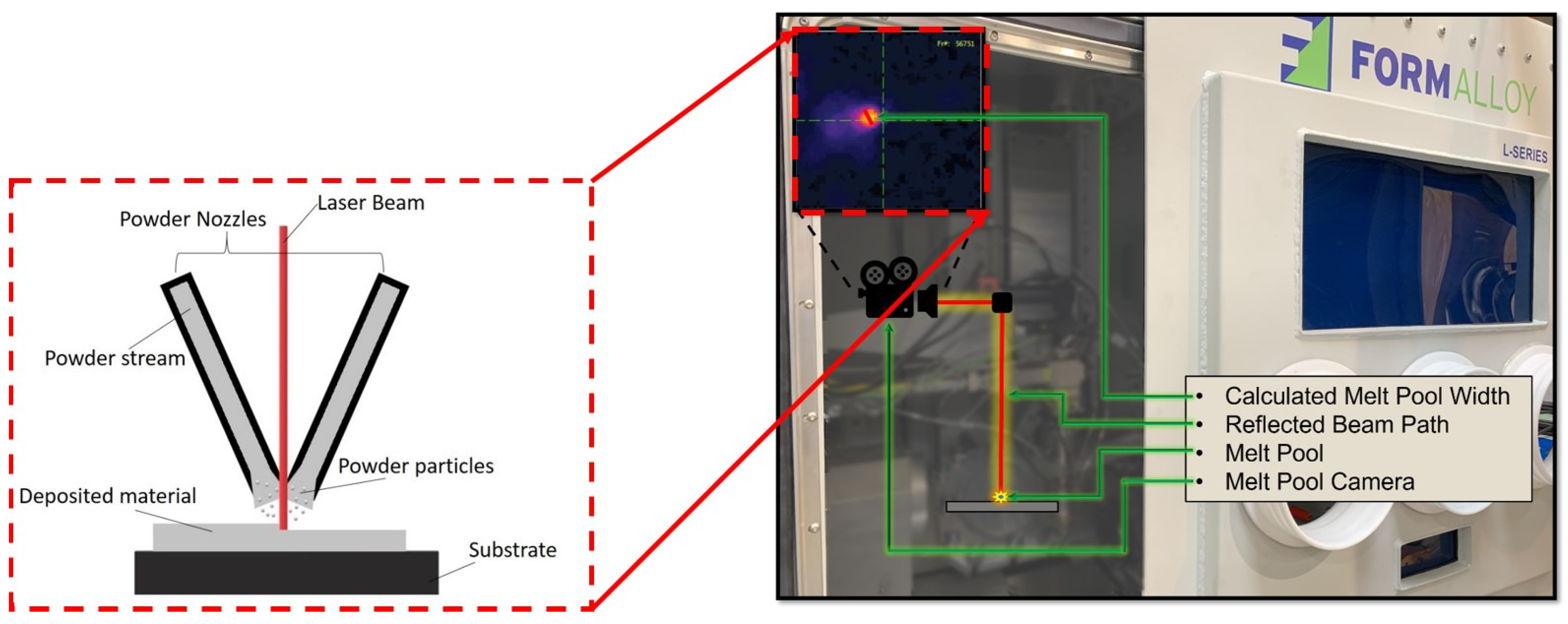
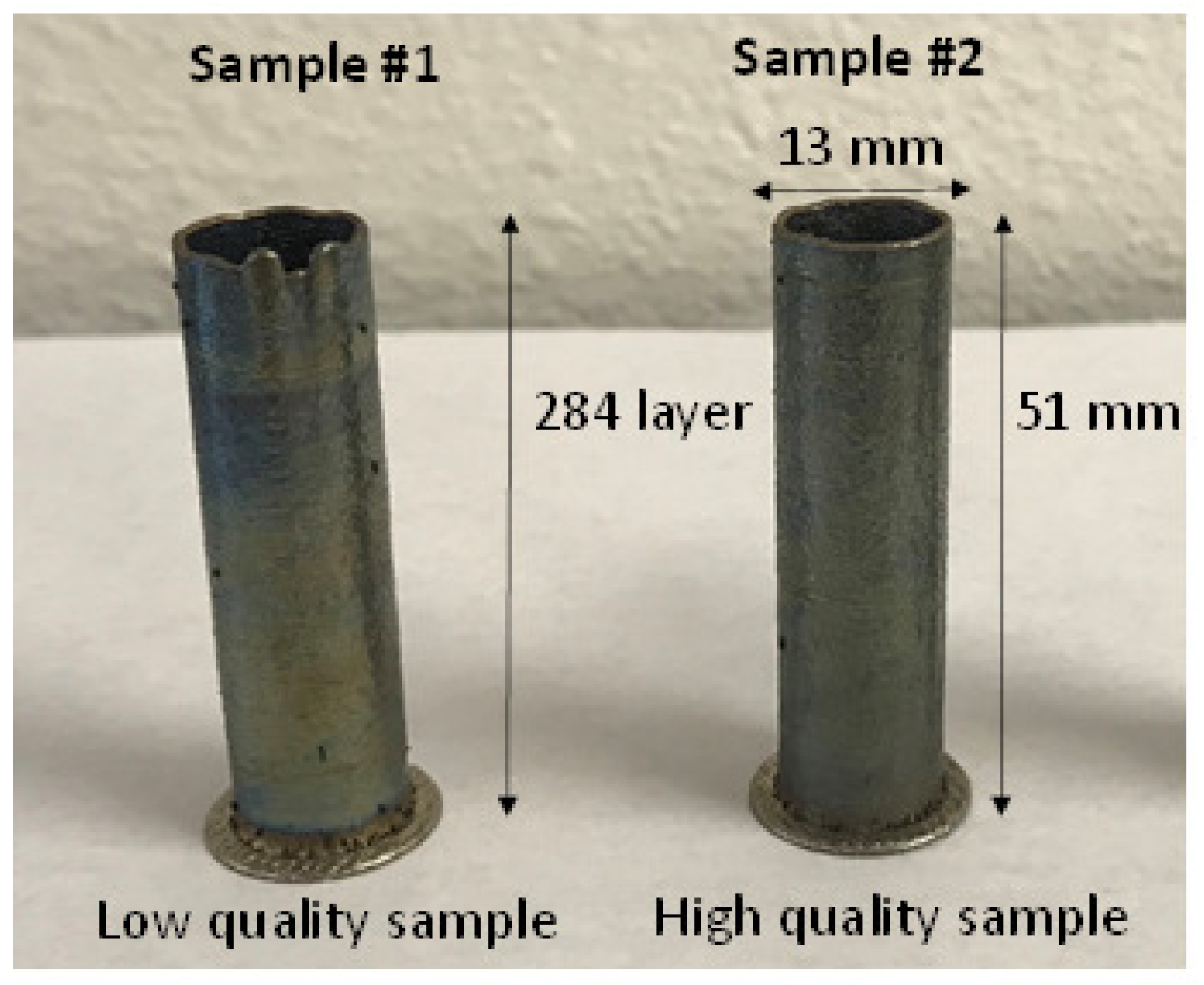

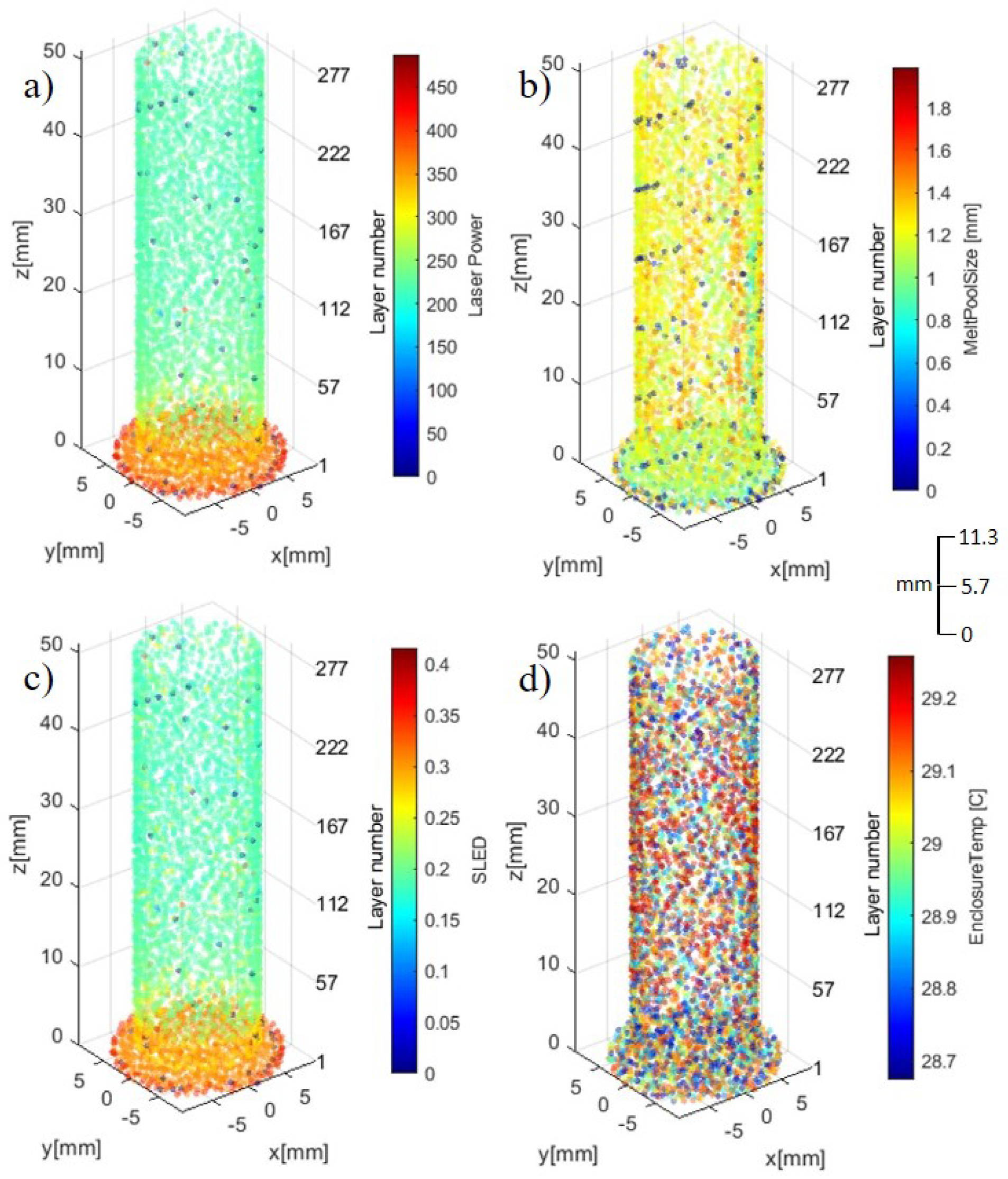

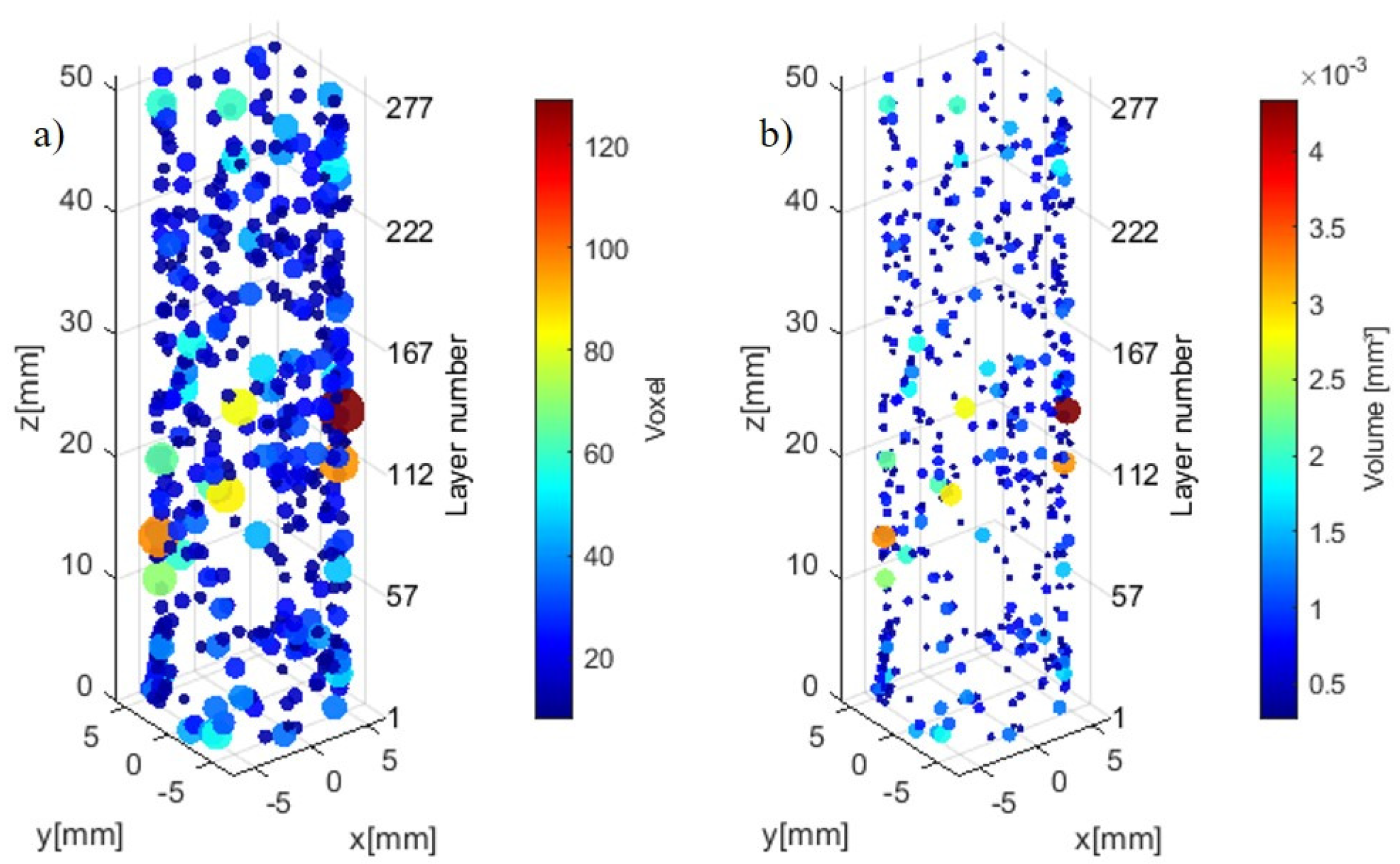
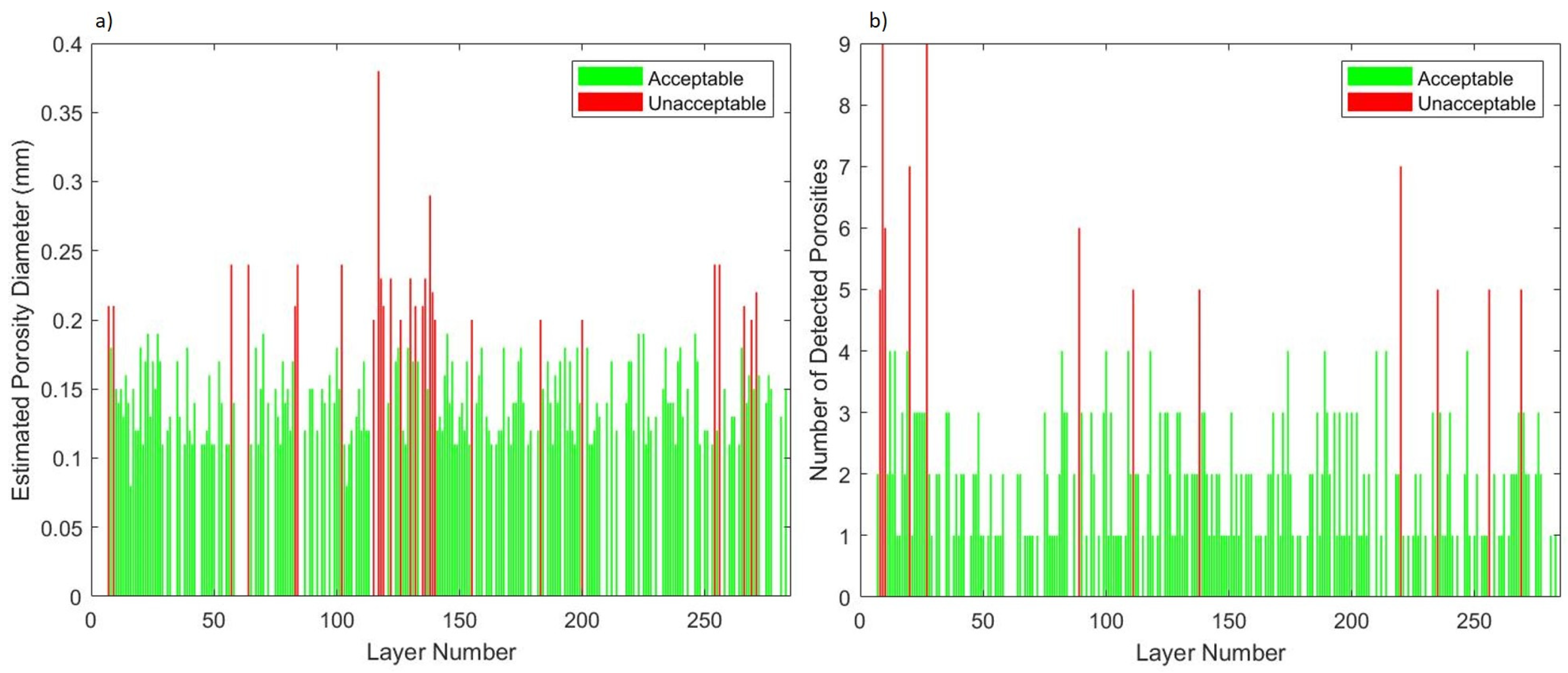
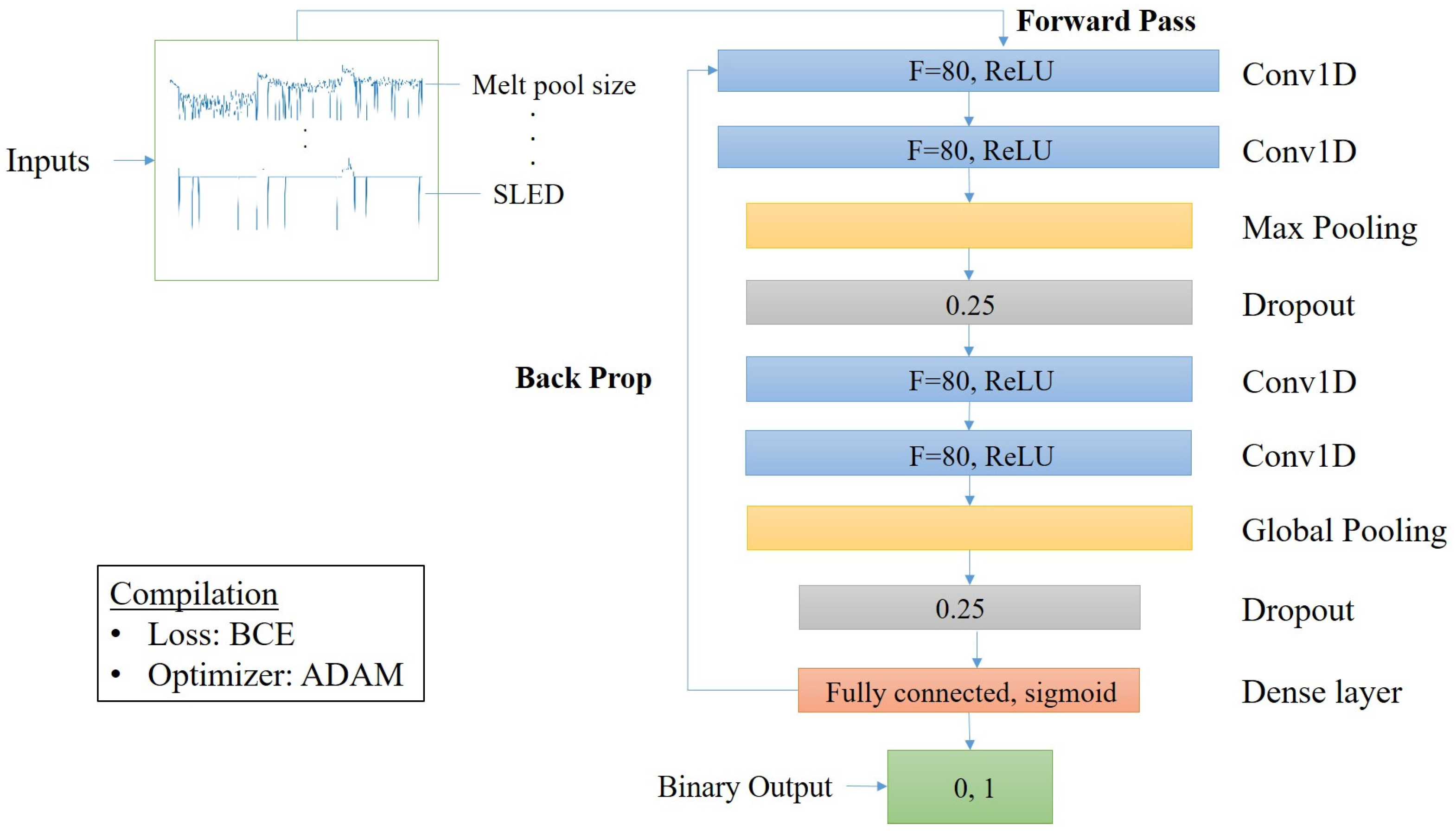
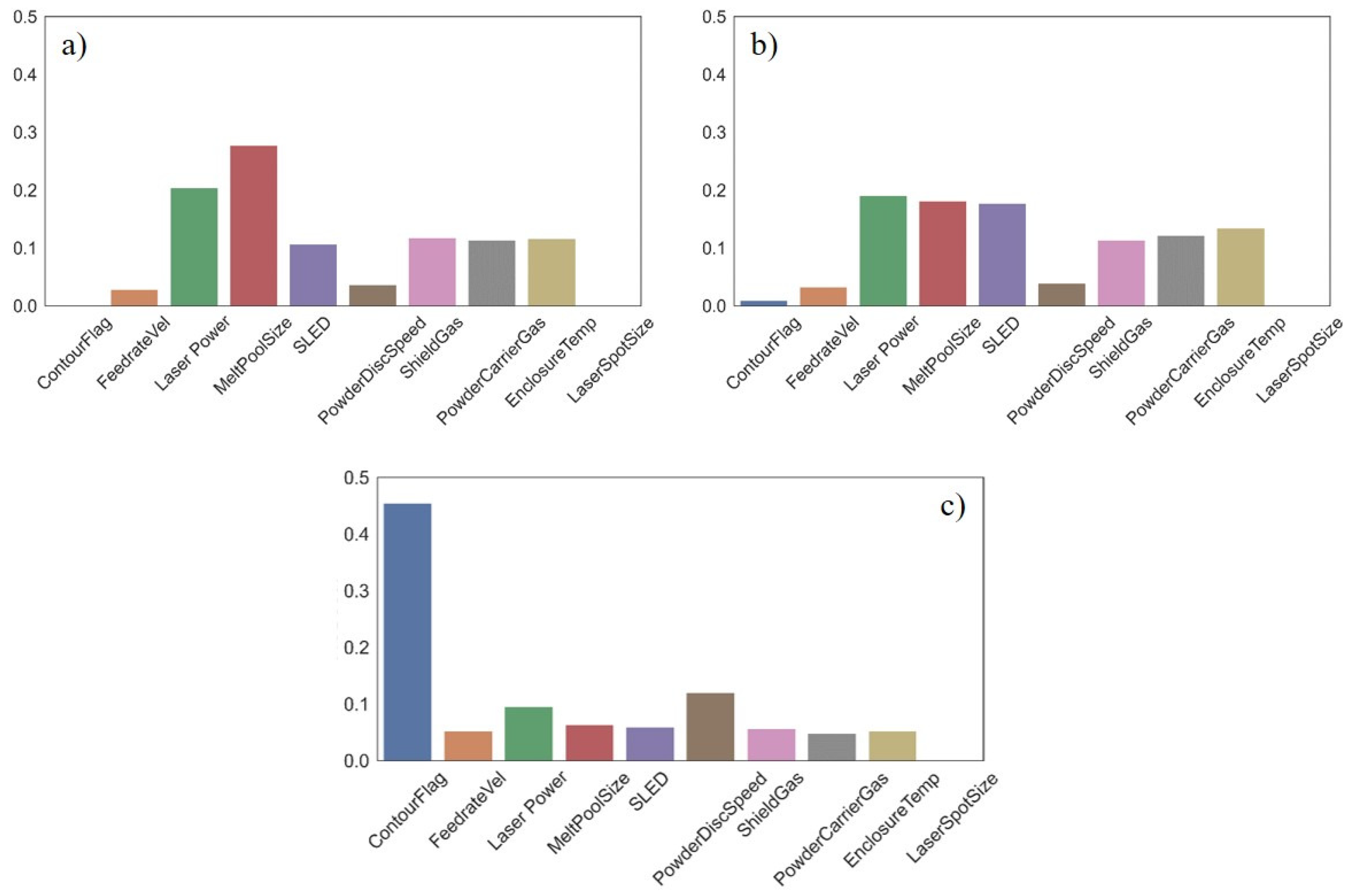
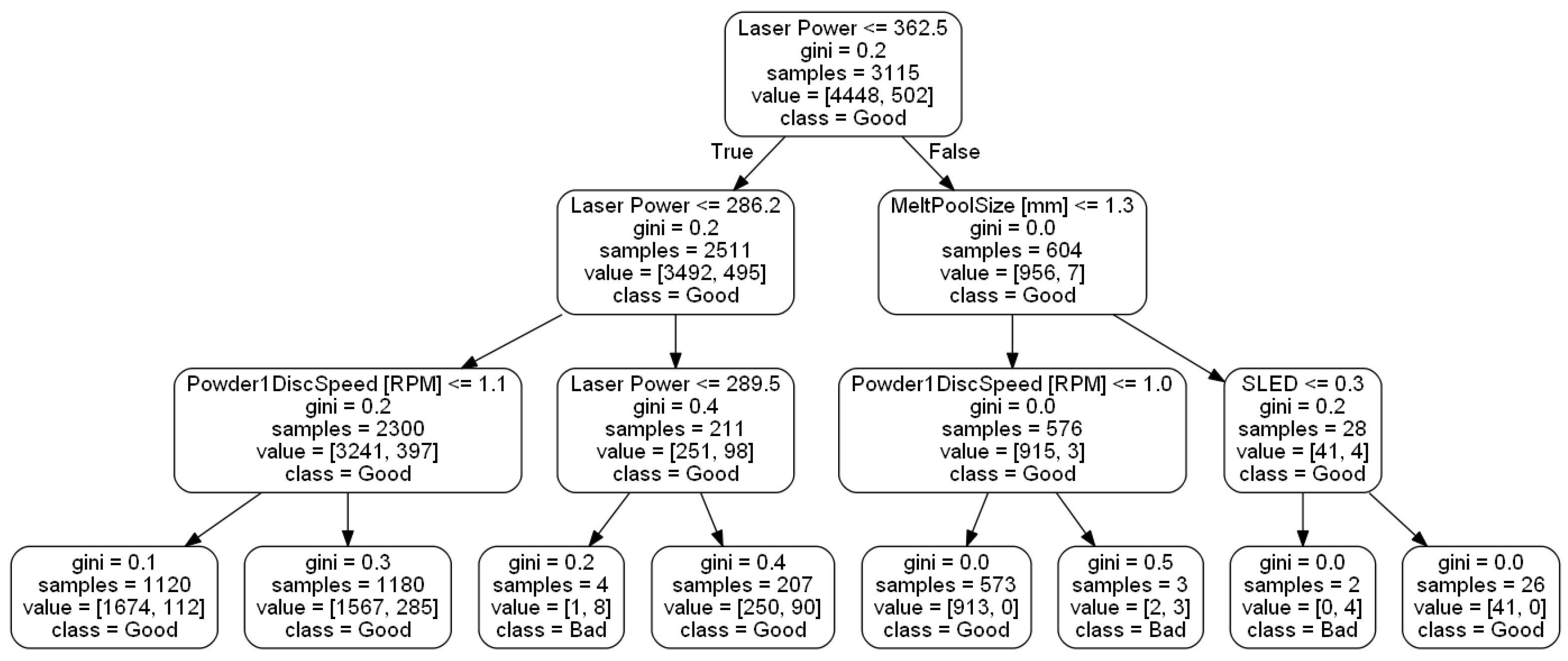
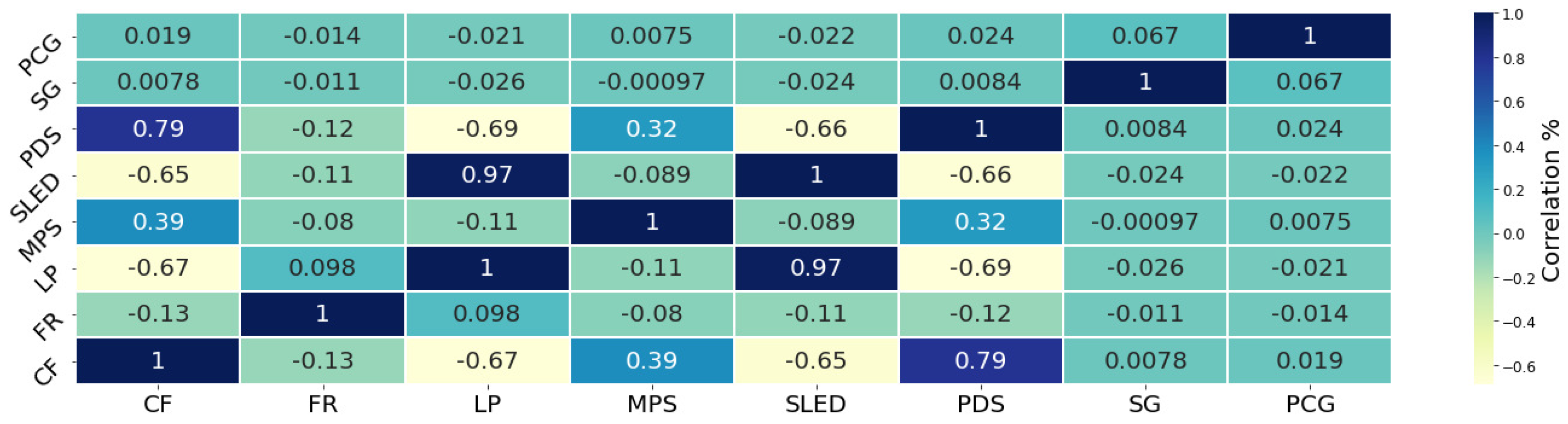
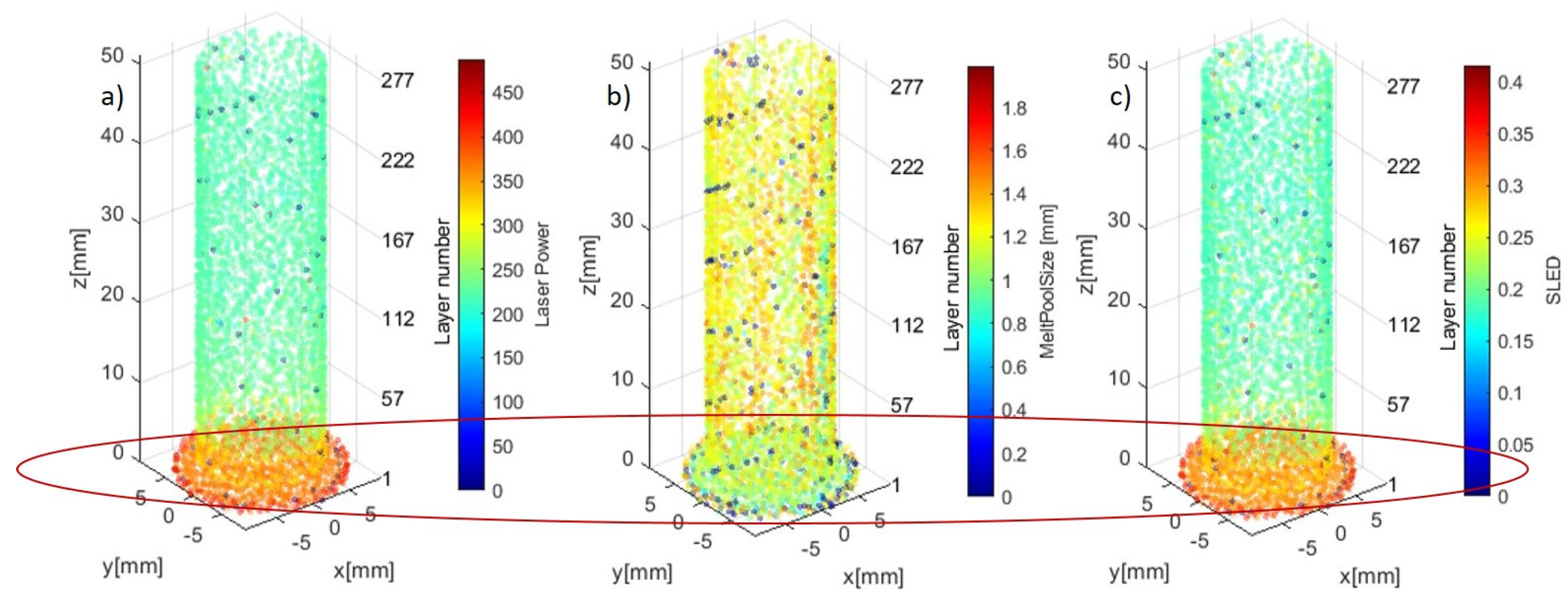
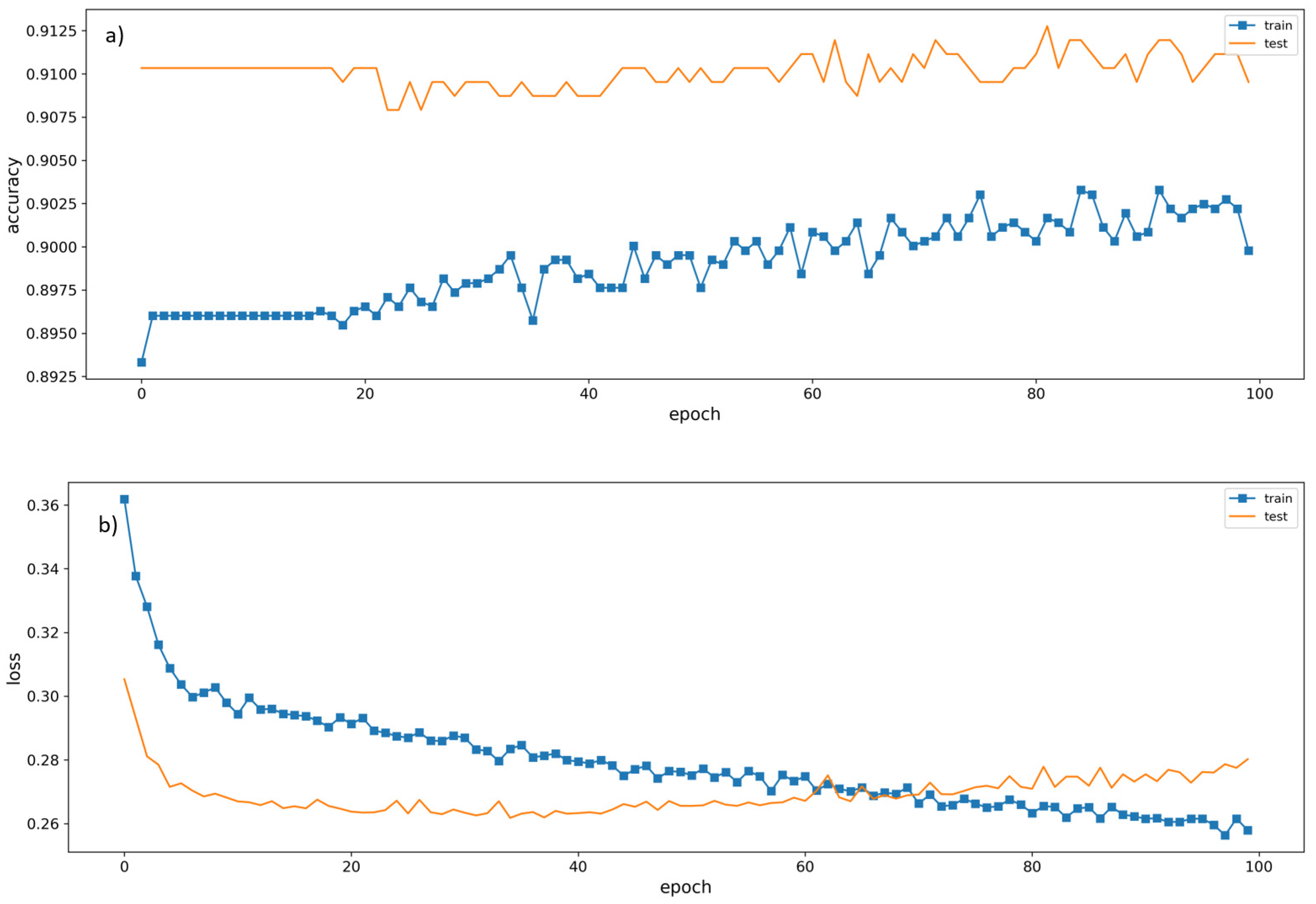
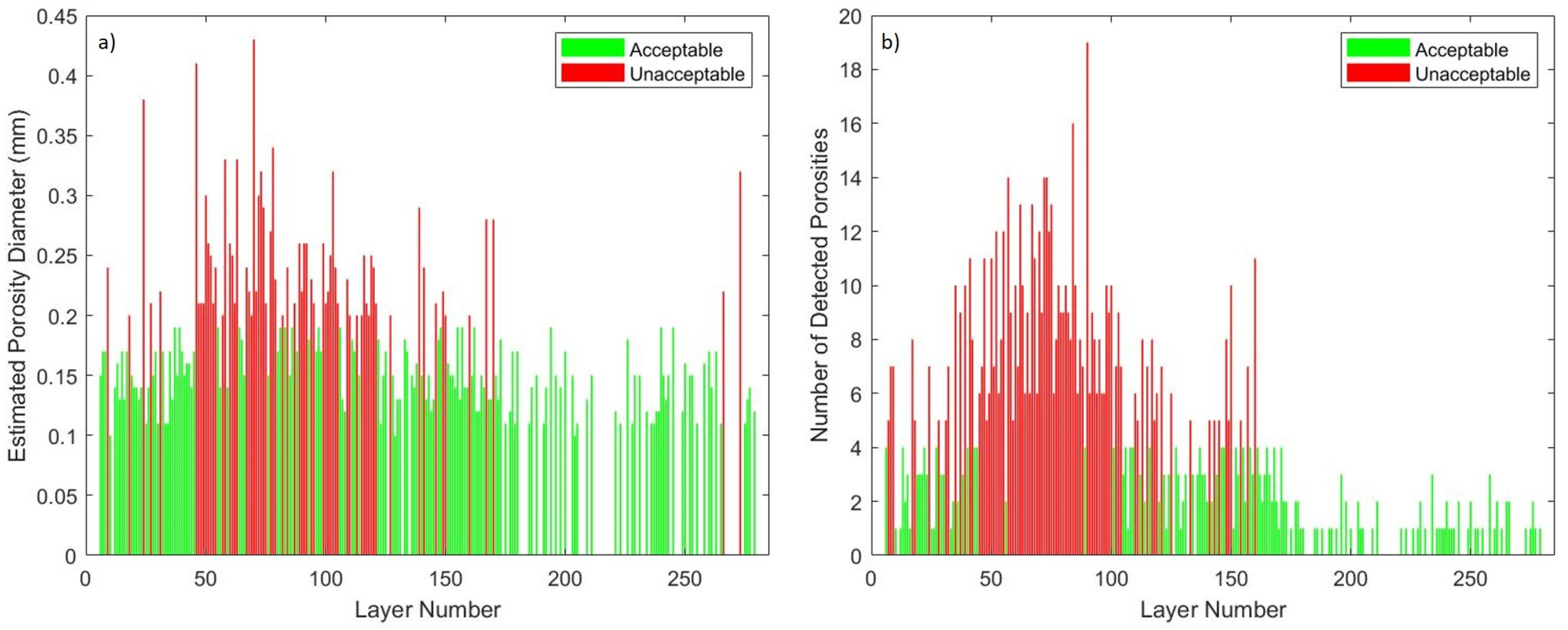
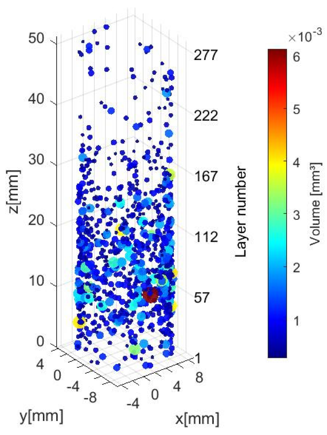

Publisher’s Note: MDPI stays neutral with regard to jurisdictional claims in published maps and institutional affiliations. |
© 2022 by the authors. Licensee MDPI, Basel, Switzerland. This article is an open access article distributed under the terms and conditions of the Creative Commons Attribution (CC BY) license (https://creativecommons.org/licenses/by/4.0/).