Analyzing Demand with Respect to Offer of Mobility

Abstract

A main key success for public transportation networks is their tuning by the analysis of mobility demand with respect to the offer in terms of public transportation means. Most of the solutions at the state of the art have strong limitations in taking into account: multiple contextual information as attractors/motivations for people movements, modalities of travel means, multiple operators, and a range of key performance indicators. For these reasons, a model for analyzing the demand with respect to the offer of mobility has been studied, and the corresponding tool DORAM developed. DORAM allows to perform the analysis of alternative scenarios, as what-if analyses, when the transport service offer and the mobility demand changed in the scenario, adopting a fast-computation strategy to compare scenarios with the aim of detecting/identifying motivations of crowded conditions on stops and on the vehicles. The analysis can exploit a wide range of data sources when computing a set of key performance indicators. The DORAM solution has been defined and developed in the MOSAIC research and development project with ALSTOM and other companies. The DORAM solution is validated by using real data and conditions in the Tuscany region.

1. Introduction

Today, public transportation systems (PTSs) are essential for sustainable mobility. When the public transportation demand is not opportunely satisfied, then the citizens are forced to use private vehicles, leading to several traffic problems in urban areas, such as traffic congestion and detection [1,2,3] and greenhouse gas (GHG) emissions in vehicles from combusted fuel, which are usually estimated by emission factors [4,5]. Providing efficient public transportation services requires policies that stimulate commuters to use services (e.g., travel time reliability [6,7], travel cost [8]). It is vital for policymakers and mobility operators, city authorities (e.g., municipalities), and infrastructure providers to be thoroughly aware of critical problems (e.g., determining crowded stops, detecting crowded time interval(s) for a stop, crowded lines) that could negatively impact on the satisfaction level of the service. To this end, to perform an extensive analysis of PTSs is essential. It has to include the analyzing of the service offer, provided by the mobility operators, with respect to the mobility demand, which refers to city users with different mobility motivations (commuters, citizens, students, etc.); with the aim of discovering what extent of the mobility demand is met by the sustainable transportation offer, which are the critical conditions, what is going to happen if something is changed in the offer/demand, etc.

A comprehensive analysis of PTSs has to provide enough flexibility by accessing, organizing, and digesting multiple data sources related to the service offers and the mobility demand. The main service-offer data can be provided in the form of General Transit Feed Specification (GTFS) [9] file format [10], which includes several fields (e.g., mobility operators: railways, ferry, tram, metro, etc.; transportation modalities, the schedule of trips); it might not be always provided by the mobility operators. The mobility demand data can be formalized in terms of origin-destination matrices (ODM) (e.g., [11,12,13]), which in turn can be obtained from different resources (e.g., fare collection using ticket validation [10] or smart cards [11], boarding/alighting passengers [8,13], census data, on board units of insurances, mobile phone data from the telecom operators, mobile phone data from mobile app operators providing navigators, census data, etc.) that are difficult or at least very expensive to have [13]. A certain amount of demand may be satisfied and oriented to exploit the public transportation offer, while others are oriented in using several kinds of private travel means: cars, bikes, motorbikes, etc. To this end, it is necessary to evaluate plans and strategies, including soft (e.g., incentives, providing information and feedback [14]) and hard ones (e.g., changing frequency of trips, ticket price, and line path [15]), designed to improve the efficiency of the offered services [13]. For instance, when complaints are received by a mobility officer about periodic crowding conditions on a bus line or on a (set of) segment(s) which connect(s) specific stops, the necessary actions to resolve the issue could include performing some on-site analysis, and then implementing possible solutions. Therefore, several solutions to the problem could not be socially, and/or economically efficient. Moreover, making modifications and verification to existing infrastructures may take a long time [16]. Therefore, to avoid ineffective on-site modifications, it is crucial to make a deep analysis to understand the impacts of changes in the current status (in most cases called Actual Scenario) of the public transportation system. Furthermore, the analysis of public transportation services, when alternative scenarios are defined by introducing a (set of) change(s) in the Actual Scenario, requires investigating a large amount of data both for the service offer and the mobility demand, and contextual changes in the road graph, when possible.

1.1. Related Works

The analysis and simulation of people flow in smart cities attracts attention due to related applications in urban mobility (e.g., [17,18,19,20,21,22,23,24,25,26,27,28]). For example, in [17], the tracking travellers’ data are collected by means of public transport IC cards and they have been modelled to predict human mobility, using three approaches. In the first two, it is assumed that the probability of passengers’ drop-off on bus line stops follows a standard or a uniform normal distribution (quite unrealistic). In the third approach, the stops have been labelled as “large”, “medium” and “small”, with respect to the numbers of passengers that are exchanged. Then, the probability of drop-off at a stop has been considered following the labelling strategy, based on the idea that larger stops attract more passengers, and as a result, the probability of drop-off at them is higher. A model for analyzing the dwell time of a bus, which is the time where a bus is stopped at a stop to exchange passengers, has been proposed in [18]. For this, the boarding and the alighting behavior of passengers, considering respectively time intervals between successive records of tapping-ins and tapping-offs, are investigated. The idea of using tapping-off information may not be applicable when onboard passengers are not obliged to tap off when they disembark at the stop. A method for the evaluation of the quality of stop alighting and boarding has been presented in [19]. One part of the mentioned research focuses on predicting the alighting stops of a stage considering a multiple-stage trip by finding the closest stop to the boarding stop of the next trip stage. A method to estimate passenger flow in real-time modality for bus transit urban systems has been proposed in [20]. In this case, the number of people picked up at a station with a smart card is estimated according to two consecutive taping records. Then, using regular commute patterns, the passengers’ alighting stations are estimated. Finally, after an estimation of the passengers’ number in real-time on a bus trip, the evaluation of onboard passengers’ number is considered by using Kalman. Otherwise, real-time mobility demand fluctuations by adopting schedule adjustments including, holding, and speed changing, has been studied in [21]. Based on a combination of big data sources and primary data, a methodology to evaluate the total trips amount to be reallocated, while considering passenger waiting time and trip cost, has been presented in [22]. A non-linear optimization model to optimize train timetables by analyzing the actual passenger loading time periods and waiting times, when records from fare collection systems are considered as a data source, has been proposed in [23]. Innovative solutions related to customized busses (in China) are analyzed in [24]. In this case, the demand estimation is performed by using the information provided by users via online platforms, in a dynamic interactive manner between operators and users, while feedbacks are exchanged among them in each step. A scheduling model to generate a timetable by realizing trade-offs among the train utilization, waiting time, energy consumption, and service levels, has been proposed in [25]. A model to estimate suitable elapsed time thresholds between sequential trip stages to identify transfers using onboard sensors, smart card fare payment data, and intermittent surveys by mobility operators is considered in [26]. A methodology to analyze comfort in PTSs, considering acceleration and vehicle vibration effects (based on international standard ISO standards) has been proposed in [27].

A visual interactive analytics system, called MobiSeg, has been proposed to support the movement activities exploration of people by analyzing taxi trajectories, telco data, and metro passenger RFID card data in [28]. There are a few works in the literature focusing on analyzing the impact of changes made in people flow (e.g., [15,29]). For example, some options to provide the mobility operators a simple way to obtain a new transport demand model are explored in [15]. The what-if analysis, which is performed by a transport planning software (called OmniTRANS), is focused on changing the frequency of trips, ticket price, and line path. What-if analysis tools are adopted to perform simulations of complex city subsystems on the basis of specific scenarios/hypotheses in order to provide support to decision makers about strategic or tactical plans. Furthermore, what-if analysis to evaluate how changing some variables (e.g., peak frequency, peak hour speed, and the distance between stops) in bus rapid transit systems can change their standards is used in [29]. Most of the discussed works assume tracking data of passengers (e.g., using public transport cards) is available, which is not realistic. They did not consider the presence of multiple mobility operators and focused on a single mode, except [28] (which focuses on Taxi and Metro) [15,17]. Moreover, they do not provide a public web-based tool to visualize the analysis results which supports REST APIs and GTFS data feed (except [12]). There are various tools for simulating people flow. For example, the open-source MatSim [30] is a multi-agent framework designed to simulate transport networks, supporting several transportation modes. Furthermore, SUMO [31] is an open-source traffic simulation package for demand modelling which considers various traffic management topics. TRANSIMS [32] is an open-source transportation model that aims at creating an integrated environment for the analysis of transportation systems. Other research introduced mobile phone data into urban analysis. For example, the AllAboard tool, which analyzes mobile phone data to visually explore urban mobility and optimize public transport, has been presented in [33]. The discussed tools, while focus on a single mobility operator (except [33]), do not support what-if analysis when creating alternative scenarios to be compared with Actual Scenario. Additionally, the user cannot access the analysis results using a web-based interface that supports GTFS data feed (except [30,33]) and REST APIs.

1.2. Paper Aims and Structure

In the present paper, a model and tool for analysis the mobility demand with respect to the public transport offer, called DORAM (Demand versus OffeR Analyzer for Mobility), is presented. The main research contributions of this paper are (a) the formal mathematical model DORAM to analyze the mobility demand with respect to the public transport offer taking into account a range of contextual and operative data, (b) the DORAM tool implementation and general strategy. DORAM solution allows operators at the city to:

• investigate how the demand is satisfied in terms of public transportation mobility by the offer considering model, simulation tools and KPIs (key performance indicator, e.g., drop-offs and pick-ups at a stop) and related evidence information (e.g., passing lines in every time interval, passing lines in each time interval) with the aim of identifying crowded condition on bus-stops and on the busses.
• Taking care in the model: (i) a range of data sources. People flow depends on different aspects (e.g., the time of day, the motivation of people for travelling, the structure public transportation network, places that with high impacts on mobility patterns). Therefore, using a wide spectrum of data sources related to the city structure (e.g., roads, stop locations), the mobility demand considering different places (e.g., residential areas, shopping centers, stadiums), and the service offer (e.g., the number of vehicle trips and lines passing the stops) supports a deeper analysis of PTSs, and as a result, more precise decisions about mobility policies; (ii) multi-modality. Multiple travel modes which permit to consider different public transportation modalities; (iii) multi-operators. It provides the analysis of the transportation network when there are multiple mobility operators; (iv) KPIs to objectively assess the alternative scenarios and making a (set of) decision(s) to improve the service offer considering the mobility demand.
• perform what-if analysis by analyzing the impact of a (set of) change(s) in Actual Scenario to see their effects in terms of people and matching demand/offer.

Changing the offer and demand in the scenarios of analysis. Performing what-if analysis by comparing the alternative scenarios with respect to Actual Scenario, which describes the current status of PTS.

DORAM provides non-functional features such as (i) flexibility, by taking into account different data sources, (ii) fast-computability, quickly switch between different scenarios, and (iii) web-based, accessing DORAM on (www.snap4city.org/odanalyzer/ accessed on 5 September 2022). Summarizing, DORAM admits some technical innovations with respect to other similar tools at the state of art that are recalled in the previous paragraph. Such features can be briefly sketched and compared in

Table 1. Related works table focus on features tools at the state of art.

Selected Tools at the State of the Art	Web-Based Interface That Supports GTFS Data and REST APIs for Analysis Results	Multi-Modal Mobility Application	Multiple Mobility Operators Applications	What-If Analysis Performance
DORAM (present work)	Yes	Yes	Yes	Yes
MATSim [30]	Yes	Yes	No	No
SUMO [31]	No	Yes	No	No
TRANSIMS [32]	No	Yes	No	No
OmniTRANS [15]	No	Yes	Yes	Yes
MobiSeg [28]	No	Yes	Yes	No
AllAboard [33]	Yes	Yes	Yes	No

, where technical aspects are considered regarding: the range of supported data, multi-modality mobility, multi-operators’ mobility and the possibility to adopt what-if analysis performance in PTSs also by using KPI.

The DORAM validation has been performed using Tuscany regional data in the Metropolitan area of Florence. Florence is the region capital with more than one and half million inhabitants, 30 million tourists per year, 1500 stops, 25 lines, and 1100 vehicle trips. DORAM is developed in a research project context, called MOSAiC [34], founded by the Tuscany Region in Italy and having important international partners as, DISIT Lab, Municipia/Engineering, CNIT, ALSTOM and TAGES. DORAM exploits the Km4City (www.km4city.org, accessed on 5 September 2022) knowledge model [35] and the Snap4City (www.snap4city.org, accessed on 5 September 2022) services [36,37].

The work has the following organization. In Section 2, we present requirements and contextual data to be considered for providing an efficient and effective framework for the analysis of mobility demand with respect to the offer of public transportation services. In Section 3 the DORAM architecture is described. Section 4 provides the model and the method to analyze the mobility demand with respect to the public transport offer, also presently the most relevant cases addressed in the model. Section 5 describes features and services provided by the DORAM. Section 6 provides the most relevant details of the solution and its validation on Actual Scenario in the area of Florence with ATAF (that is, the transport company of the Florence area, in Italian “Azienda Trasporti Autolinee Fiorentine”), with the aim of identifying crowded condition at the bus stops and on the busses. ATAF is one of the main mobility operators in the Tuscany region. The analysis took into account 25 lines (which is 21.92% of the total in Florence) 11,173 trips (16.67% of the total in Florence), and 942 stops (62.26% of the total in Florence). Finally, in Section 7 conclusions are considered.

2. Data Source and Requirements Analysis

DORAM provides a model and tool for analyzing PTSs by comparing the service offer with respect to mobility demand. In this regard, the main requirements are presented and discussed in this section.

Req.1: matching/analyzing the mobility demand with respect to the offer in terms of public transportation means, taking into account: multiple operators and modalities.

Req.2: changing the offer and the demand in the scenarios. Performing the so-called what-if analysis by analyzing the impact of a (set of) change(s) in Actual Scenario to see the effects in alternative scenarios. Changes to the offer aims to verify if they may better satisfy the demand and can be automatically composed producing random changes around the present solution and taking a direction of action. Changes in the demand may be provoked by city changes, for example, the construction of a new stadium, the creation of 300 new apartments and entertainment services in a former industrial area.

Req.3: computing a number of KPIs (e.g., drop-offs and pick-ups at a stop) and related information (e.g., passing lines in each time interval) which may allow to make a decision about the solutions proposed in changes at the offer. The most relevant aspects to be measured among the others are related to the number of people: (i) at the stops/stations to reduce the overcrowded situations, to improve the quality of service and for safety reasons; (ii) on the travel means (vehicles: busses, train, metro, ferry, cages, etc.) to reduce the overcrowded situations, to improve the quality of service and for safety reasons.

Req.4: exploiting a range of data sources which may increase precision in the computational model, related to: the city structure and services, demand of mobility, sharing services. Please note that city structure and services may provide information to understand motivations to the city users to move. For example, a large residential area is a source of people in the morning, and an attractor during the late afternoon; a large shopping center, a stadium, a park area, and other attractors. See for example the study regarding the typical city user behavior in the different parts of the city [38], where the usage of Wi-Fi access points data permitted to understand the people flows and to reconstruct origin destination matrices for hour of the day in the week, over than 300 observation points.

The Data Sources to perform the analysis are in accordance with the characteristics of the city (e.g., available transportation modalities, presence of tourists). In particular, the main aspects of service offer can be obtained by considering provided services in terms of public transportation networks for moving in the city which may be obtained from (1) GTFS data, which includes different related information according with mobility operators, transportation modalities (e.g., intercity bus, city bus, ferry, tram, train), vehicle planned trips (e.g., paths, time tables), (2) eventual real-time vehicle positions, which could be not easy to obtain, and (3) alternative transportation modalities (e.g., car sharing, bike sharing). Furthermore, the mobility demand can be computed to obtain origin destination matrices by considering a large data range:

• census data which includes the mobility (and the public transportation means) of residents from/to the city for different purposes (e.g., work, study);
• traffic flow which includes counting (private) vehicles entering or exiting from the city over time which is typically performed on the city border using different methods (e.g., plate number recognition);
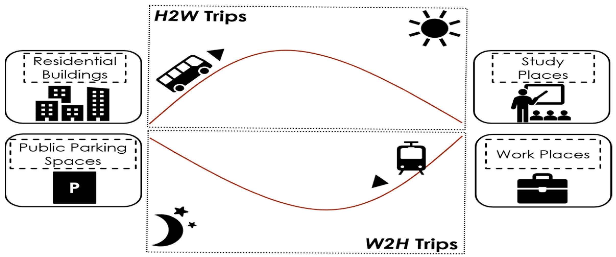
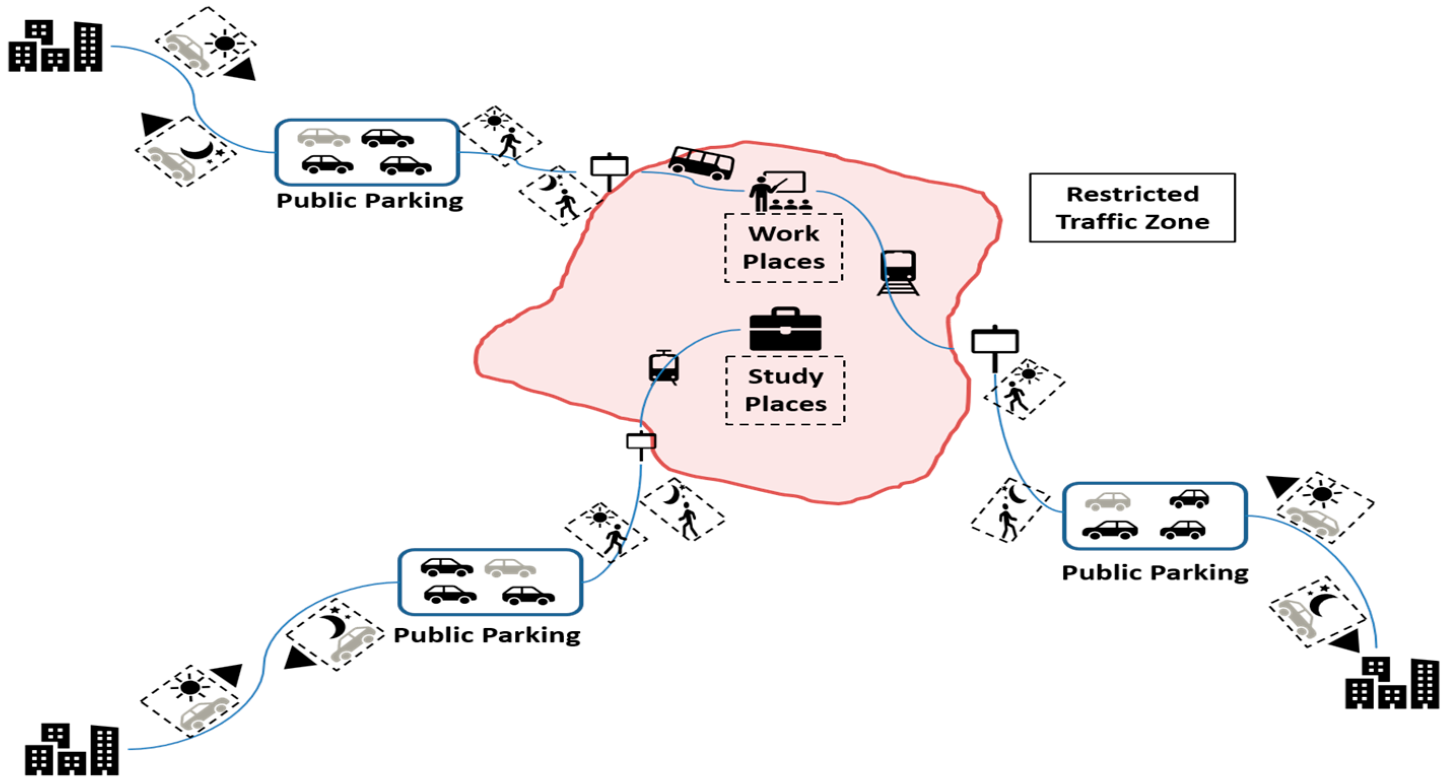
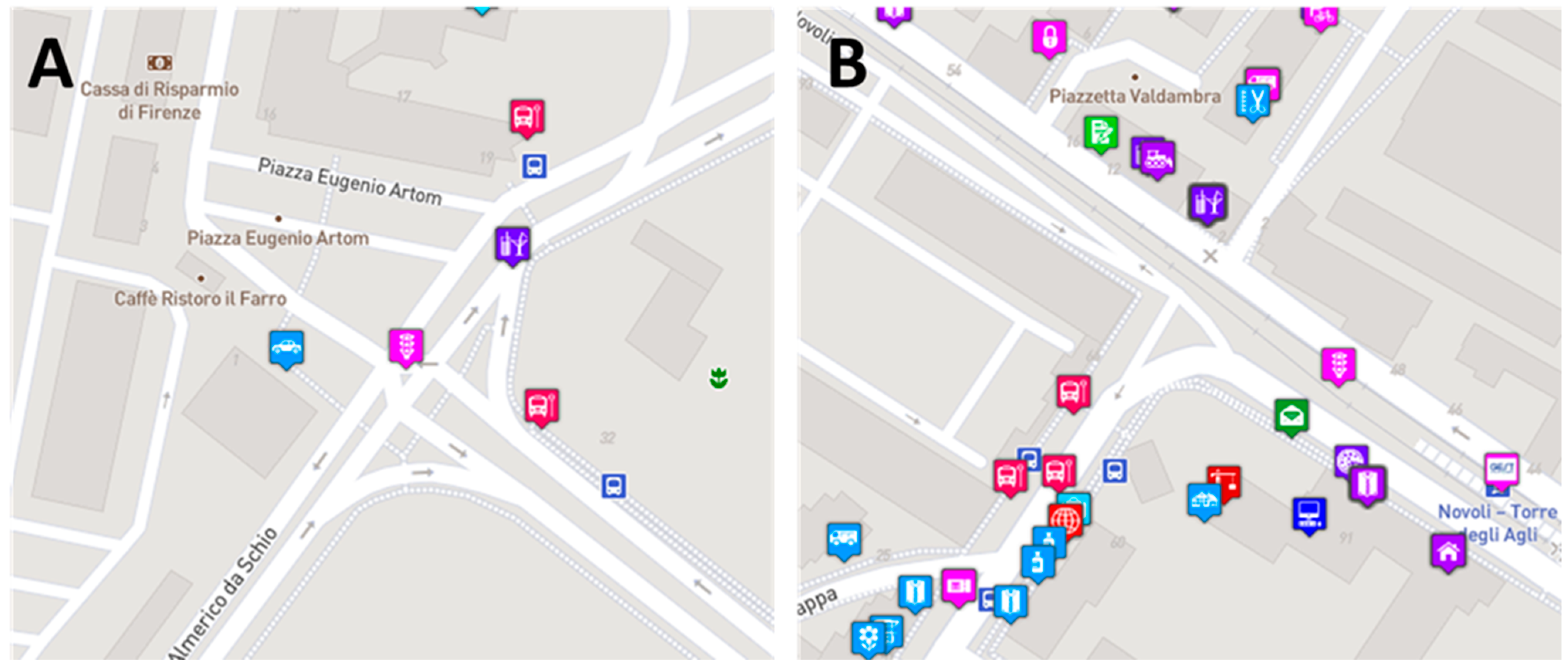
• city structure and services attract city users depending on daytime. For example, in the morning, residential areas and public parking spaces can be starting point of trips because the city users usually start from these places to go to work and study places and return in the late afternoon. Likewise, in the afternoon, service providers (e.g., offices, stores, industries, schools, shopping malls, touristic places).
• commuter flows in the city which can be obtained using different data sources (e.g., Wi-Fi, network cellular, mobile applications, PAXCounter);
• commuter flows accessing the city. For example, in cities (e.g., Venezia, Roma, Firenze) that the presence of tourists cannot be neglected compared to others (e.g., workers, students), data that come from cellular [39] or Wi-Fi [38] networks, can help to analyze different aspects (e.g., the number of tourists that are daily present in the city, the duration of their stay, their origin and destination in long term/distance).
• deployed transportation services which can be achieved using different methods (e.g., counting the commuters onboard, waiting at stops/stations, in multimodal hubs, exiting from railway stations over time).

Therefore, the proposed model and tool have to provide enough flexibility to take into account those data source in modelling the service offer and the mobility demand. However, the analysis of the service offer with reference to the mobility demand requires processing a considerable volume of data which is a time-consuming process and could take several hours or even days. In order to provide the analysis of different scenarios it is necessary to have a fast model and to produce results in short time, and to provide them in a visual analytic tool.

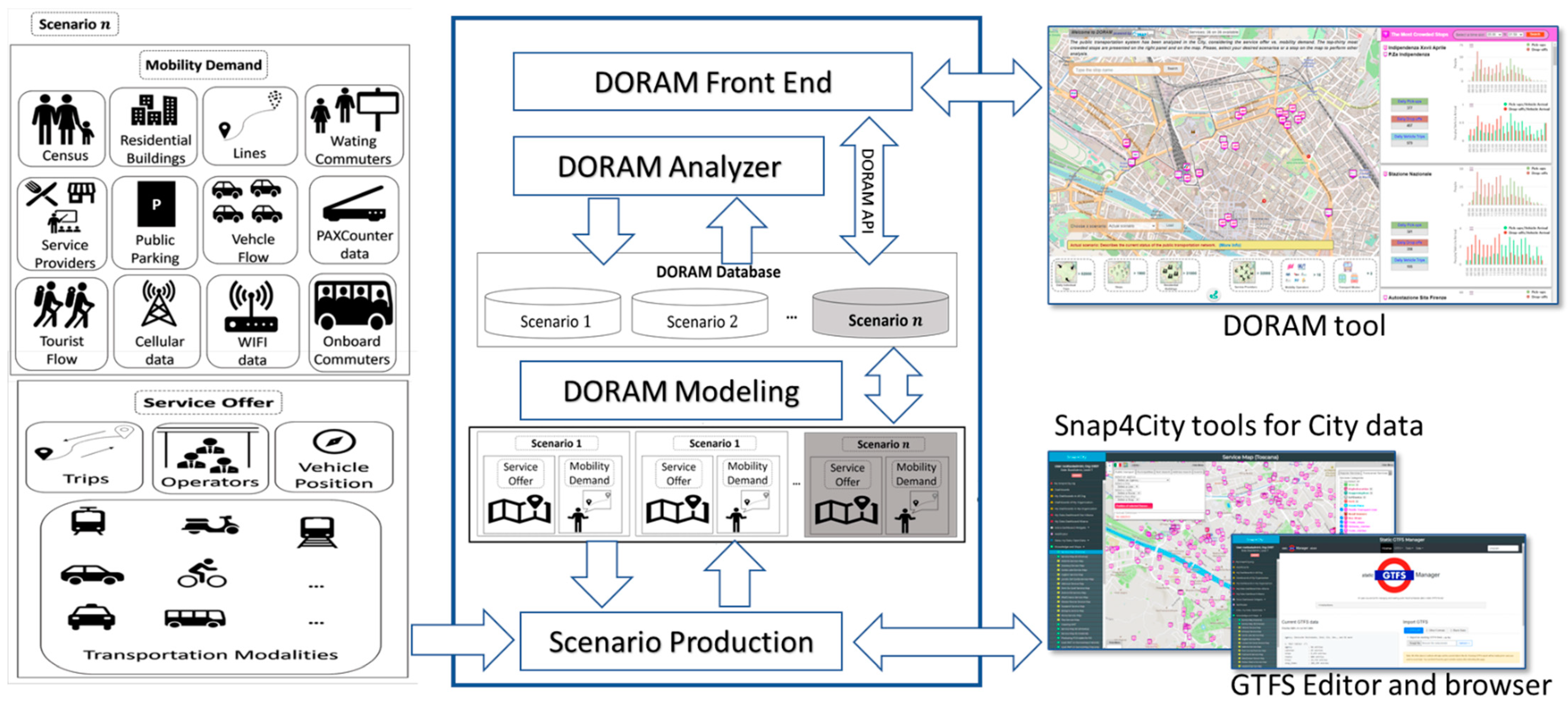
3. DORAM Architecture

The DORAM solution aimed at satisfying the above requirements, and it is based on the architecture reported in Figure 1, with components:

• Scenario Production. A new scenario is created by aggregating different kind of data. The Scenario model is formalized in a knowledge base NoSQL RDF Storage with all the city relationships and services are modeled. In particular: (i) to load/change/create a transport offer in the so called static GTFS manager (GTFS) has been used to edit an existing GTFS data feed, (ii) Snap4City OSM2SM tool allowed to retrieve the residential building data from OpenStreetMap (OSM) [40] database and save them in a PostgreSQL database, (iii) census data, which includes different categories (e.g., daily resident flow from each locality to another for work or study, the daily tourist flow), retrieved from various sources (e.g., [41,42]), (iv) Points Of Interest (POI) data, retrieved using ServiceMap of Snap4City [43].
• DORAM Modelling takes the scenario information to define the simulation and relating the data, associated with service offer and the mobility demand, and the simulation output, as described in Section 4.
• DORAM Analyzer performs the analysis of the public transportation system by comparing the mobility demand and service offer. In order to do that, the scenario data are retrieved using ServiceMap APIs calls and SPARQL queries performed on Snap4City/Km4City knowledge base [44] provided for each scenario in a separated Docker (e.g., [41,42]).
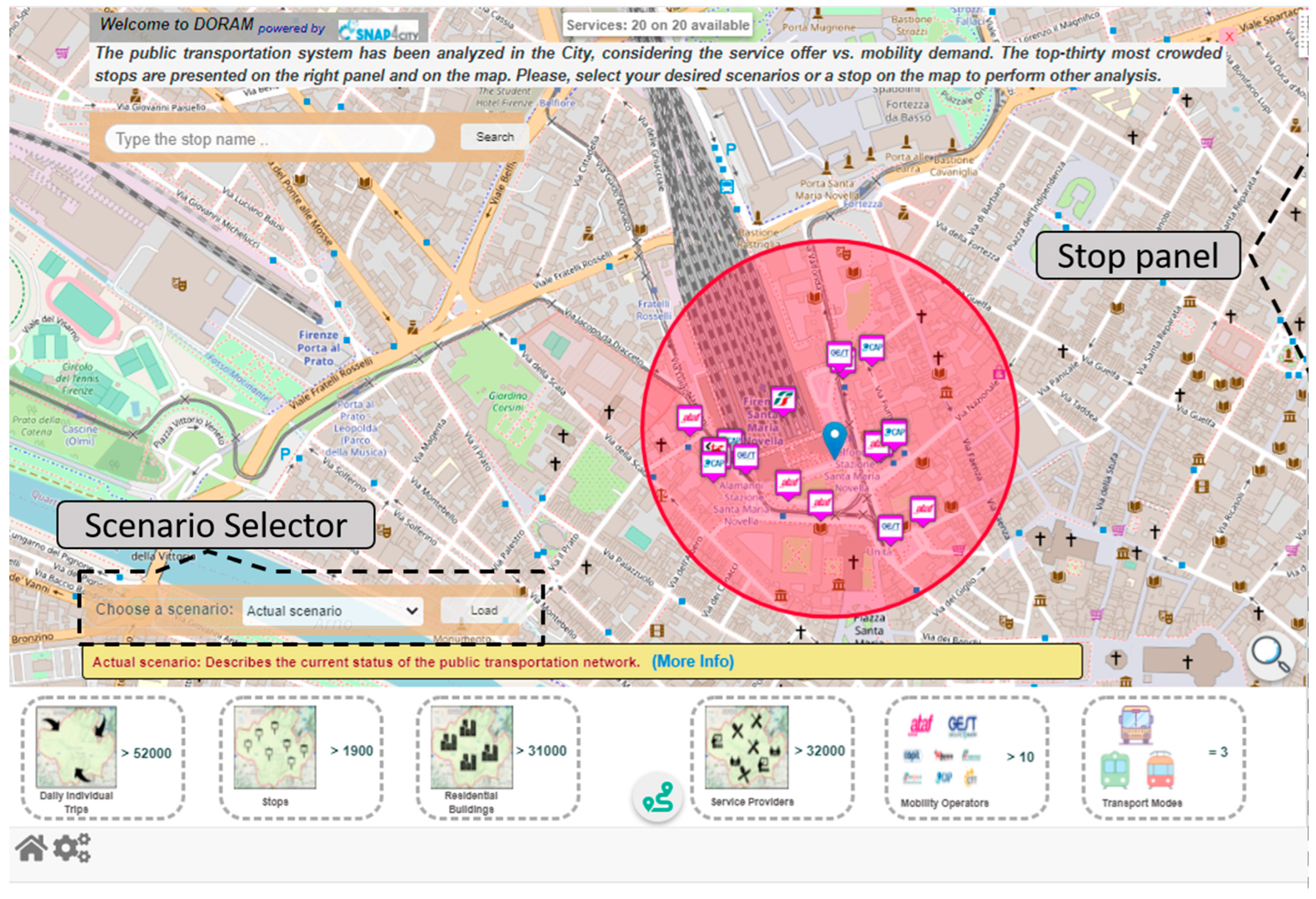
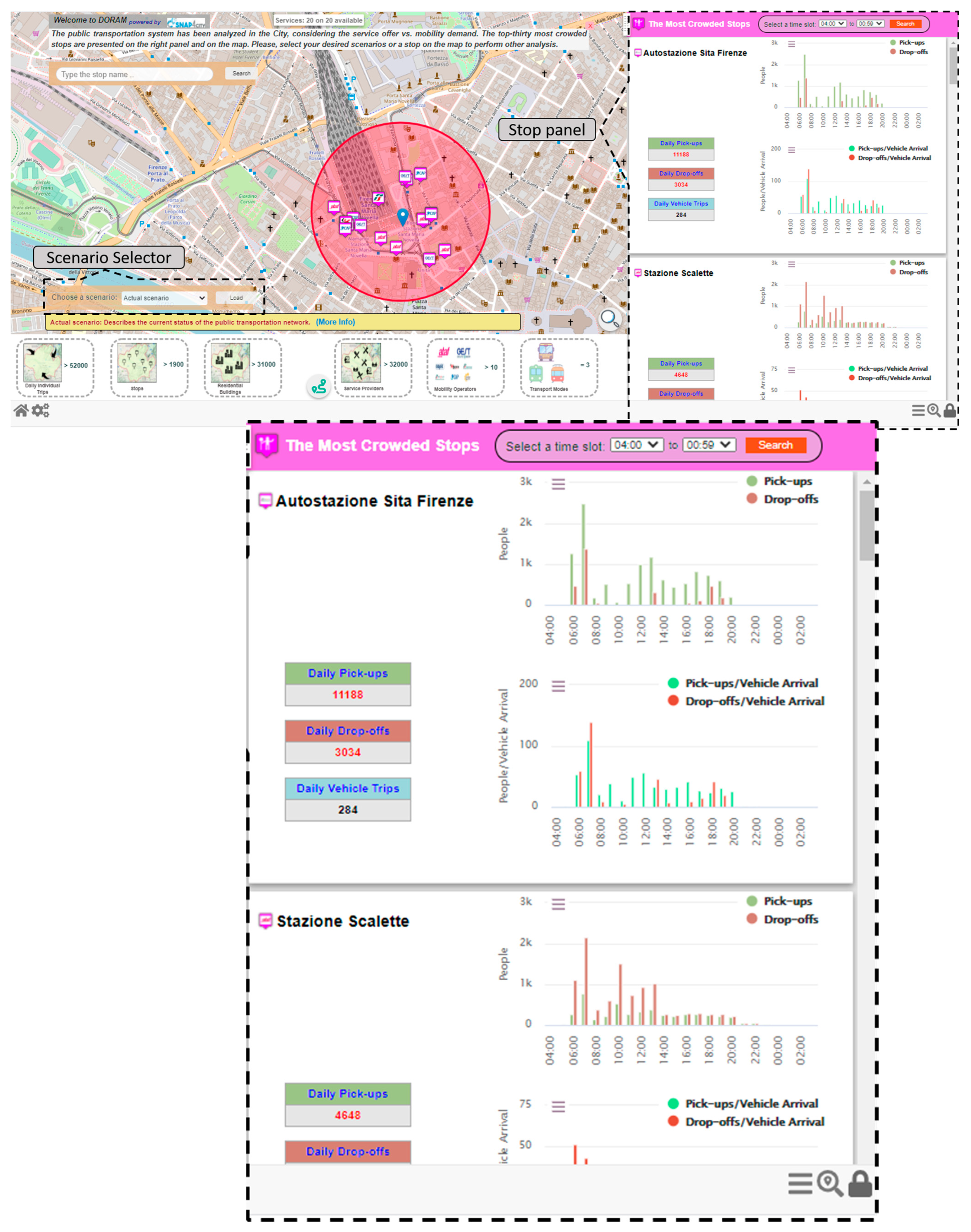
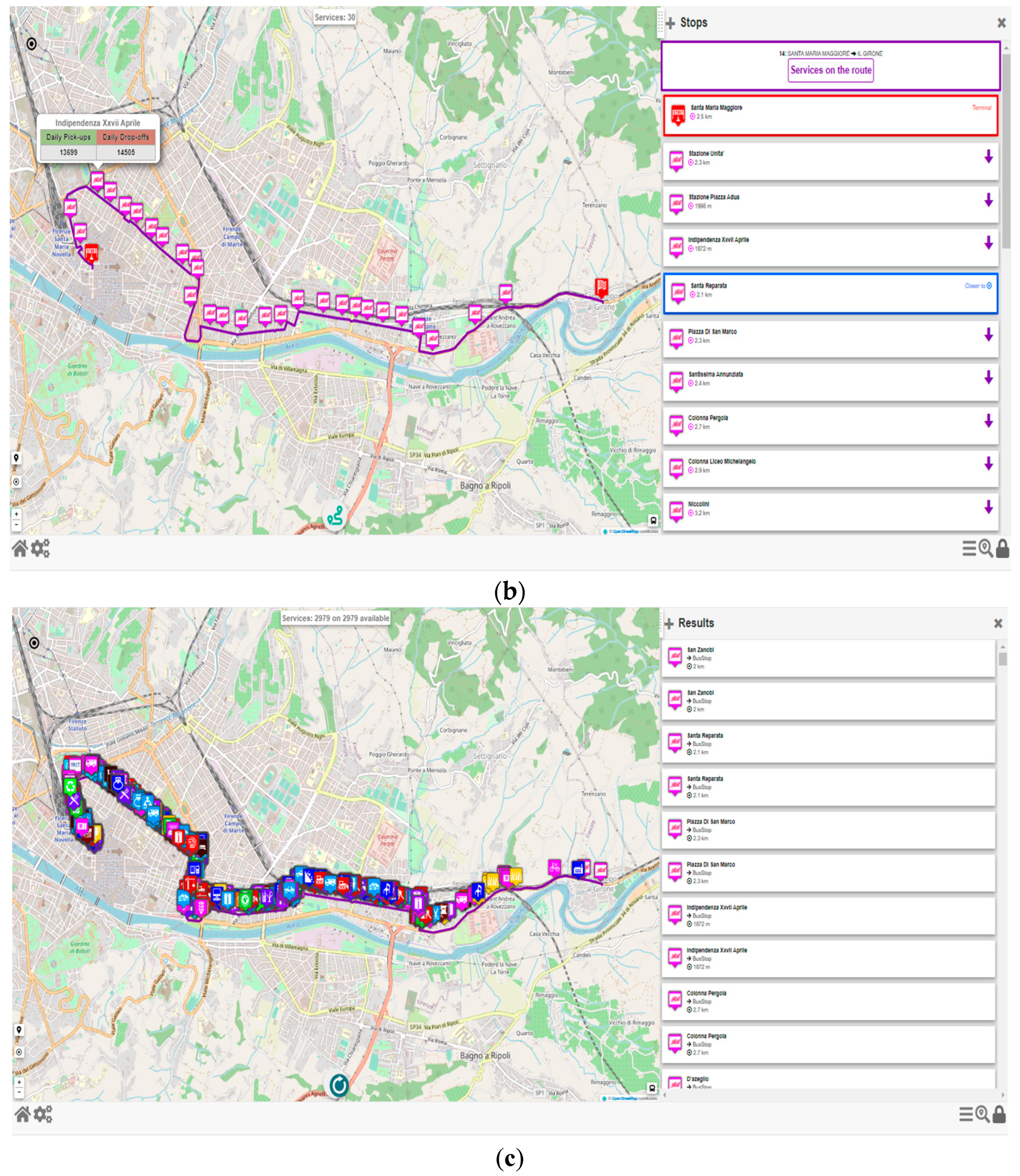
• DORAM Front-End allows to (i) select the scenario to be analyzed, (ii) browse the scenario by navigating in the transport offer (bus stops, lines, time schedule, start stops, etc.), (iii) browse the city areas to see the services and point of interests, (iv) analyze the results of each scenario.

4. Model and Analyzer

In this section, we describe how the service offer and the mobility demand are modelled in DORAM. Then, how they are compared by analyzing two main KPIs (i.e., the picked up and dropped number at a stop in a given time interval).

4.1. Modelling Public Transport Service Offer

The modelling of public transportation services from offered side by a (set of) mobility operator(s) should lead to evaluate the people number moving from a location to another. In turn the movement of people can be re-produced in the form of an offered Origin-Destination Matrix (ODM) for various time slots. The goal is to verify if people demand is satisfied by means of the service planning of the public transport. Therefore, we have considered the time set $T=\left\{mng, aft\right\}$, for the two main time slots in working days (morning ($mng$) and afternoon ($aft$)). In

Table 2. Main formal notations.

Notation	Description
$s$	A given bus stop
$M$	$\mathrm{Mobility} \mathrm{modality} \mathrm{set} ({e}.{g}., M=\left\{bus, tram,train\right\})$
$\mathbb{O}$	$\mathrm{Mobility} \mathrm{operator} \mathrm{set} ({e}.{g}., \mathbb{O}=\left\{ATAF,GEST,TRENITALIA\right\}$)
$T=\left\{mng,aft\right\}$	Time set
$t$	A given time in $T$
$k$	The $k\text{-}\mathrm{th} \mathrm{time} \mathrm{interval} \mathrm{in} t\in T$
${{𝕥}}_{i,j}\left(t, m,\mathrm{𝕠}\right)$	$\mathrm{Number} \mathrm{of} \mathrm{vehicle} \mathrm{trips} \mathrm{in} \mathrm{time} t\in T$$\mathrm{with} \mathrm{mobility} \mathrm{modality} m\in M$
$c\left(m,\mathrm{𝕠}\right)$	Vehicle capacity with modality m and mobility operator $\mathrm{𝕠}$
$\mathbb{P}$	$\mathrm{Service} \mathrm{provider} \mathrm{set} ({e}.{g}., \mathbb{P}=\left\{Office,Public university, Shopping mall\right\}$)
$O\left(t\right)$	Offer by means ODMs
$D\left(t\right)$	Demand by means ODMs
$L$	Set of locations in the region R
$L^{\prime }\subset L$	Set of locations in the area A
$In\left(t\right)$$\mathrm{and} Out\left(t\right)$	Number of inbound and outbound individual trips
$pick\left(mng\right)and$$pick\left(aft\right)$	$\mathrm{Total} \mathrm{morning} \mathrm{and} \mathrm{afternoon} \mathrm{pick}\text{-}\mathrm{ups} \mathrm{in} \mathrm{the} \mathrm{studied} \mathrm{area} A$
$drp\left(mng\right)and$$drp\left(aft\right)$	$\mathrm{Total} \mathrm{morning} \mathrm{and} \mathrm{afternoon} \mathrm{drop}\text{-}\mathrm{offs} \mathrm{in} \mathrm{the} \mathrm{studied} \mathrm{area} A$
$s_{beg}, s_{tra},$$\mathrm{and} s_{fin}$	Beginning, Transfer and Final stops in a commuter trip
$c\left(s,r\right)$	Circle with stop s in its center and related radius r
$W_{md}$	Modality weight vector
$W_{pr}$	pr (parking, residential buildings) weight vector
$W_{\mathrm{sp}}$	Service provider weight vector
$H\left(t\right)$	$\mathrm{Time} \mathrm{interval} \mathrm{vector} \mathrm{for} t\in T$
$W\left(t\right)$	$\mathrm{Weight} \mathrm{vector} \mathrm{associated} \mathrm{with} \mathrm{time} t\in T$
${\alpha }_{stp}\left(s,t,k\right)$	Stop level of stop s in interval time $H\left(t\right)\left[k\right]$
${\alpha }_{lin}\left(s,t,k\right)$	Line level of stop s in interval time $H\left(t\right)\left[k\right]$
${\alpha }_{pr}\left(s\right)$	pr (parking, residential buildings) level of stop s
${\alpha }_{sp}\left(s\right)$	Service provider level of stop s
$u_{tra}^{\left(stp\right)}\left(s,t,k\right)$	stop weighted sum of stop s in interval time $H\left(t\right)\left[k\right]$
$u_{pr}\left(s\right)$	pr (parking, residential buildings) weighted sum of stop s
$u_{sp}\left(s\right)$	Service provider weighted sum of stop s
$P_{tra}^{\left(stp\right)}\left(s,t,k\right)$	Probability that stop s is a transfer one by choosing other stops in circle c(s,r) in interval time $H\left(t\right)\left[k\right]$
$P_{tra}^{\left(lin\right)}\left(s,t,k\right)$	Transfer Probability of the stop s by choosing other lines of s in interval time $H\left(t\right)\left[k\right]$
$P_{tra}\left(s,t,k\right)$	Transfer Probability of the stop s in interval time $H\left(t\right)\left[k\right]$
$P_{beg}\left(s,t\right)$	Beginning Probability of the stop s in t ∈ T
$P_{fin}\left(s,t\right)$	Final Probability of the stop s in $t\in T$
$P_{tra \cup beg}\left(s,t,k\right)$	$\mathrm{Probability} \mathrm{of} a \mathrm{transfer} s_{tra}$$\mathrm{or} a \mathrm{beginning} s_{beg}$$\mathrm{stop} \mathrm{in} \mathrm{interval} \mathrm{time} H\left(t\right)\left[k\right]$
$P_{tra \cup fin}\left(s,t,k\right)$	$\mathrm{Probability} \mathrm{of} a \mathrm{transfer} s_{tra}$$\mathrm{or} a \mathrm{final} s_{fin}$$\mathrm{stop} \mathrm{in} \mathrm{interval} \mathrm{time} H\left(t\right)\left[k\right]$
$drp\left(s,t,k\right)$$\mathrm{and} pck\left(s,t,k\right)$	Drop-offs and pick-ups at stop s in interval time $H\left(t\right)\left[k\right]$
${𝕥}\left(s,t,k\right)$	Number of vehicle arrivals at stop s in time interval $H\left(t\right)\left[k\right]$

the used notations in the DORAM model are shown. The morning offer ODM $O_{\left|L\right|\times \left|L\right|}\left(mng\right)$ is defined by means of the matrix having in the cell $O_{i,j}\left(mng\right)\left(O_{i,j}\left(aft\right)\right)$ the total number of people moving from locality $l_i$ to $l_j$, in the morning time (afternoon time). Formally, the cells $O_{i,j}\left( t\in T\right)$ are calculated as in (2).

$$O_{i,j}\left(t\right)={\displaystyle \sum }_{m=1}^{\left|M\right|}{\displaystyle \sum }_{\mathrm{𝕠}=1}^{\left|𝕆\right|}{{𝕥}}_{i,j}\left(t, m,\mathrm{𝕠}\right). c\left(m,\mathrm{𝕠}\right)$$

(1)

where ${{𝕥}}_{i,j}\left(t, m,\mathrm{𝕠}\right)$ denote the number of vehicle trips with mobility modality $m\in M$ (e.g., bus, tram) and mobility operator $\mathrm{𝕠}\in \mathbb{O}$ (e.g., ATAF, Busitalia) from locality $l_i$ to locality $l_j$, in $T=\left\{mng,aft\right\}$. Moreover, c$\left(m,\mathrm{𝕠}\right)$ denotes the vehicle capacity with modality $m$ and operator $\mathrm{𝕠}$. The operator $“.”$ denotes the multiplication between scalars.

4.2. Modelling Mobility Demand

The city users move for different motivations, for the resident commuters, work and study can be considered as two main motivations. The trips of resident commuters can be divided into two sets (see Figure 2).

First, Home to Work trips (H2W) which lead to study or workplaces. They usually start from home, in the morning. Furthermore, the commuters with private vehicles, usually park them in public parking spaces when the work or study places are located in restricted traffic zones, and then, start a H2W trip from there to reach their destination, using the public means of transportation. Second, Work to Home trips (W2H), which lead to home in the afternoon. They usually start from work or study places. Typically, the commuters, with private vehicles, who work or study in the restricted traffic zones start a W2H trip (see Figure 3). This behavior has been observed in census data collected by Tuscany Region of all the inhabitants.

For a region $R$ (Tuscany region for example), including a set $L$ of locations, the (morning) demand ODM $D_{\left|L\right|\times \left|L\right|}\left(mng\right)$ is defined by means of the matrix containing in cell $D_{i,j}\left(mng\right)$, the total amount of outbound trips in H2W. Likewise, the (afternoon) demand ODM $D_{\left|L\right|\times \left|L\right|}\left(aft\right)$ is considered as the transpose of the demand matrix $D_{\left|L\right|\times \left|L\right|}\left(mng\right)$ in the morning. That is, $D\left(aft\right)=D^{\left(T\right)}\left(mng\right)$, where the operator $T$ denotes the transpose, and the cell $D_{i,j}\left(aft\right)$ describes the number of outbound trips in W2H, from location $l_i$ to $l_j$. It is noted that the demand matrices $D_{\left|L\right|\times \left|L\right|}\left(t\right)$ are defined considering all modalities in $M$ and all mobility operators in $\mathbb{O}$. Note that commuters who go to a given studying or working place during the morning time, usually return home during the afternoon time. Then, the number of outbound trips in W2H from location $l_i$ to $l_j$ is equal to the number of inbound trips in W2H to locality $l_j$ from $l_i$ (i.e., $D_{i,j}\left(mng\right)=D_{j,i,}\left(aft\right)$). Such an assumption is primarily considered for residential commuters, and the model can be also applied to transitory flow since it depends on the collected data from different sources as mentioned in the previous description, and such data take into consideration the presence of tourists/events also. Commonly, residential commuters’ flows are only considered during working days. In this case, a stationary/conservative behavior is defined, and it is applied to the model by means of Equations (2) and (3). For an area $A$ (the city of Florence is an example) in region $R$ of Tuscany Region including a set $L^{\prime }\subset L$ of locations, the flow of commuters can be defined as the total number of the outbound trips in the morning $Out\left(mng\right)$ and the inbound trips in the afternoon $In\left(aft\right)$, respectively, from and to a given area $A$. As defined in (2), $Out\left(mng\right)$ is equal to $In\left(aft\right)$ and it is evaluated by means of the sum of the total amount of the outbound trips in the morning from each location $l ϵ L^{\prime }$ to the all places in set $L$.

$$Out\left(mng\right)=In\left(aft\right)={\displaystyle \sum }_{i=1}^{\left|L^{\prime }\right|}{\displaystyle \sum }_{j=1}^{\left|L\right|}{D}_{i,j}\left(mng\right)$$

(2)

Analogously, we obtain (3)$.$

$$In\left(mng\right)=Out\left(aft\right)={\displaystyle \sum }_{i=1}^{\left|L^{\prime }\right|}{\displaystyle \sum }_{j=1}^{\left|L\right|}{D}_{i,j}\left(aft\right)$$

(3)

Without loss of generality, in the case of transitory flow involving a not stationary behavior, the model takes into account $Out\left(mng\right)$ and $In\left(aft\right)$ in Equation (2) and $In\left(mng\right)$ and $Out\left(aft\right)$ in Equation (3) which may be distinct from each other. The same solution applies for cases in which one may have unbalanced inflow/outflow for different reasons such as: football games that may provoke numerous arrivals by train, and fractioned departures in the following days, etc.

We analyze the service offer with respect to the demand, in the form of the offer $O\left(t\right)$ and demand $D\left(t\right)$ matrices. In the following, we present our approach on how we compared service offer and mobility demand, considering the dropped off and picked up numbers at a stop.

4.3. Service Offer with Respect Mobility Demand Computation

DORAM aims to analyze the transportation networks by investigating to what degree the offer satisfies the mobility demand. To do that, two main KPI are used: (1) pick-ups count and (2) drop-offs count at each stop $s$ because they describe the service suitability (under-provision or over-provision) at s. For example, when $50$ vehicle trips pass through a stop, $2000$ people in a specific time slot should be picked up (or dropped off) indicates that the service is under-provisioned, while $20$ pick-ups (or drop-offs) indicates that the service is over-provisioned, at the stop. The perfect rate depends on the restrictions and bus size. To analyze the trend of the daily pick-ups and drop-offs at stop $s$, it is required to evaluate the motivation of the commuters to move. The commuters stage-wise (see Figure 4) consider two types of trips to reach their destination: (1) single-stage trip, taking only one vehicle x trip and (2) multi-stage trips, taking multiple vehicles. A stop then can be a (i) beginning stop ($s_{beg}$), (ii) final stop ($s_{fin}$), or (iii) transfer stop ($s_{tra}$).

4.3.1. Paper Aims and Structure

We considered two parameters that affect drop-offs and pick-ups at a transfer stop $s_{tra}$: stop density and vehicle line frequency which are formal defined as follows.

Stop density. Since the number of stops near a stop $s$ increases, then the probability that $s$ is a transfer stop $s_{tra}$ is higher since more commuters can select $s$ to transfer according with the next trip by moving to a close stop in multi-stage trips. For example, Figure 5 shows the differences about the stop density in stops $\mathrm{A}$ and $\mathrm{B}$.

Stops/stations may have different mobility modalities (e.g., bus, tram, train), in a modality set $M$, and may have similar motivations as transfer. For example, a train station is typically a strong point of start in the city to go to work/study, and to go back, compared to a bus/tram stop, which in some cases are city transfer. Thus, we defined a modality weight vector $W_{md}\left[1,\dots ,\left|M\right|\right]$, where stops/stations with higher modality weight have a higher potential for being a transfer $s_{tra}$. For example, if $W_{md}=\left[0.9,0.05,0.05\right]$ and $W_{md}\left[train\right]=0.9$ indicates that, a train station has a higher potential to be a transfer one, compared to a stop ($W_{md}\left[bus\right]=0.05$). Given a circle $c\left(s,r\right)$ with stop $s$ as its center and the related radius $r$, we compute the probability that $s$, in a time interval in an interval vector $H_{t\in \left\{mng,aft\right\}}$, is a transfer one by choosing other stops in $c\left(s,r\right)$, as formally described in the following definition.

Definition 1.

Let $P_{tra}^{\left(stp\right)}\left(s,t,k\right)$ denote the probability that stop s, in interval time $H\left(t\in \left\{mng,aft\right\}\right)\left[k\right]$, is a transfer one by choosing other stops in circle $c\left(s,r\right) in interval time H\left(t\right)\left[k\right]$. It is then calculated as in (4).

$$P_{tra}^{\left(stp\right)}\left(s,t,k\right)=e^{\left(-\frac{1}{{\alpha }_{stp}\left(s,t,k\right)}\right)}$$

(4)

It is noted that ${\alpha }_{stp}\left(s,t,k\right)$ is the stop level of stop $s$ which indicates the normalized weighted sum of the number of stops in circle $c\left(s,r\right) in time interval H\left(t\right)\left[k\right]$ and calculated as in (5).

$${\alpha }_{stp}\left(s,t,k\right)=\frac{u_{tra}^{\left(stp\right)}\left(s,t,k\right)-u_{tra}^{\left(stp\right)}\left(min\right)}{u_{tra}^{\left(stp\right)}\left(max\right)-u_{tra}^{\left(stp\right)}\left(min\right)}$$

(5)

where $u_{tra}^{\left(stp\right)}\left(s,t,k\right)$ is the stop weighted sum of stop $s$ in $H\left(t\right)\left[k\right]$ and calculated as in (6).

$$u_{tra}^{\left(stp\right)}\left(s,t,k\right)={\displaystyle \sum }_{mϵM}^{\left|M\right|}{N}_{stp}\left(m,t,k\right).W_{stp}\left[m\right]$$

(6)

$N_{stp}\left(m,t,k\right)$is the number of stops with transfer modality$mϵM$in circle$c\left(s,r\right)$with at least one passing vehicle trip in time interval$H\left(t\right)\left[k\right]$. Furthermore,$u_{tra}^{\left(stp\right)}\left(min\right)$and$u_{tra}^{\left(stp\right)}\left(max\right)$respectively denote the minimum and maximum stop weighted sums, considering all stops in studied area$A.$

Vehicle line frequency. During a time interval, a higher number of lines passing near a stop/station indicates that, compared to other stops, it is more likely to be used by the commuters as a transfer $s_{tra}$. For example, Indipendenza XXVII Aprile stop (operated by ATAF) as one of the most crowded stops in the city of Florence with more than $nine$ (or $18$ in both directions) lines, is highly used as a transfer stop. Formally, we have:

Definition 2.

Let$P_{tra}^{\left(lin\right)}\left(s,t,k\right)$denote the probability that$s$ is a transfer stop by choosing other lines of$s$ in interval time$H\left(t\right)\left[k\right]$. It is then calculated as in (7).

$$P_{tra}^{\left(lin\right)}\left(s,t,k\right)=e^{\left(-\frac{1}{{\alpha }_{lin}\left(s,t,k\right)}\right)}$$

(7)

${\alpha }_{lin}\left(s,t,k\right)$ is the line level of stop $s$, which indicates the normalized number of lines of $s$, and calculated as in (8).

$${\alpha }_{lin}\left(s,t,k\right)=\frac{N_{lin}\left(s,t,k\right)-N_{lin}\left(min\right)}{N_{lin}\left(max\right)-N_{lin}\left(min\right)}$$

(8)

$N_{lin}\left(s,t,k\right)$ is the number of lines passing stop $s$ in time interval $H\left(t\right)\left[k\right]$. Furthermore, $N_{lin}\left(min\right)$ and $N_{lin}\left(max\right)$ denote the minimum and maximum line numbers, considering all stops in area $A.$ Then, the probability that stop $s$ is a transfer one $s_{tra}$ in time interval $H\left(t\right)\left[k\right]$ is defined as in (9) where the operator $“.”$ denotes the multiplication between scalars. Note that being a transfer stop by choosing other stops in circle $c\left(s,r\right)$ and by choosing other lines of $s$ are assumed to be independent because the incidence of one does not affect the other.

$$\begin{array}{c}{P}_{tra}\left(s,t,k\right)=P_{tra}^{\left(stp\right)}\left(s,t,k\right)+P_{tra}^{\left(lin\right)}\left(s,t,k\right)\\ \hfill -P_{tra}^{\left(stp\right)}\left(s,t,k\right).P_{tra}^{\left(lin\right)}\left(s,t,k\right)\end{array}$$

(9)

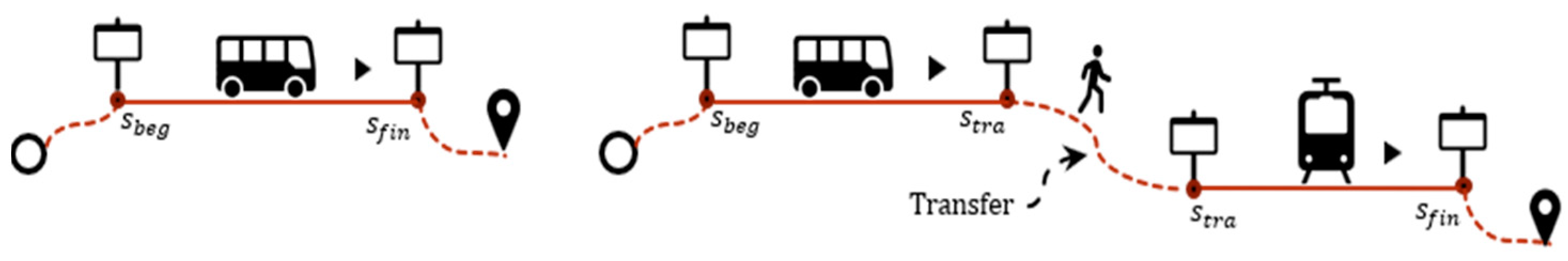
4.3.2. Beginning and Final Stops’ Analysis

We focus on some parameters when analyzing beginning $s_{beg}$ and final $s_{fin}$ stops of trips: household density, parking density and service provider density which are formal defined as follows.

Household density. Since the residential buildings density near a stop increases, then a higher number of pick-ups (drop-offs) could be considered at the stop in the morning (afternoon). More precisely, it is more expected that the commuters/city-user begin (end) their H2W (W2H) trips at the given stop in the morning (afternoon). Figure 6 shows the residential building density at the stops $\mathrm{A}$ and $\mathrm{B}$ using the Overpass Turbo tool [45].

Parking density. As above-discussed, commuters study or work places in restricted traffic zones, typically park their private vehicles in public parking spaces, and then use public transport systems to reach their destination in the morning (see Figure 3). Moreover, in the afternoon, the public transport system is used to reach the parking spaces to reach home by private vehicles. Therefore, like residential buildings, in the morning (afternoon), when the density of public parking spaces around a stop increases, more commuters can use the given stop. Since a considerable number of commuters use public parking spaces to park their private vehicles, stops around public parking spaces, compared to those around residential buildings, usually could produce and attract more commuter trips. To consider this point, we define pr (parking-residential) weight vector $W_{pr}\left[parking,residential\right]$, where a higher weight for a place (e.g., $W_{pr }\left[parking\right]=0.95$), compared to others (e.g.,$W_{pr }\left[residential\right]=0.05$), indicates that a higher number of commuters could start (or end) their H2W (or W2H) trips at a nearby stop. Formally, we have:

Definition 3.

Let$P_{beg}\left(s,mng\right)\left(P_{fin}\left(s,aft\right)\right)$denote the probability that stop$s$ is a beginning$s_{beg}$(final$s_{fin}$) one in the morning (afternoon). It is then calculated as in (10).

$$P_{beg}\left(s,mng\right)=P_{fin}\left(s,aft\right)=e^{\left(-\frac{1}{{\alpha }_{pr}\left(s\right)}\right)}$$

(10)

It is noted that ${\alpha }_{pr}\left(s\right)$ is the parking-residential level of stop $s$, which indicates the normalized weighted sum of the number of public parking spaces and residential buildings in circle $c\left(s,r\right)$, and calculated as in (11).

$${\alpha }_{pr}\left(s\right)=\frac{u_{pr}\left(s\right)-u_{pr}\left(min\right)}{u_{pr}\left(max\right)-u_{pr}\left(min\right)}$$

(11)

where, $u_{sp}\left(s\right)$ is the pr weighted sum of stop $s$ and calculated as in (12).

$$\begin{array}{c}{u}_{sp}\left(s\right)=N_{pr}\left(s,parking\right).W_{pr}\left[parking\right]\\ +N_{pr}\left(s,residential\right).W_{pr}\left[residential\right]\end{array}$$

(12)

$N_{pr}\left(parking\right)$ and $N_{pr}\left(residential\right)$ are respectively the number of public parking spaces and residential buildings in circle $c\left(s,r\right)$. Furthermore, $u_{sp}\left(min\right)$ and $u_{sp}\left(max\right)$ respectively denote the minimum and maximum $pr$ weighted sums, considering all stops.

Service provider density. There are several categories of service providers including work (e.g., offices, shopping malls) and study (e.g., schools, universities) places. As mentioned, in the morning, the city-users are supposed to go to work/study (H2W trips) and return in the afternoon (W2H trips). Therefore, when the service provider places’ density is higher near a stop s, then the probability that s is a final stop $s_{fin}$ (beginning stop $s_{beg}$) is higher since more commuters can terminate (start) the related trips in the morning (afternoon). In Figure 7. Density of services around stops $\mathrm{A}$ and $\mathrm{B}$.

Since the service density is higher in B, then we can expect that the city-users would select stop $\mathrm{B}$ as their final $s_{fin}$ (beginning $s_{beg}$) one in the morning (afternoon). Please note that not all services $\mathbb{P}$ have the same attraction. For example, a shopping mall or a public university may attract more people, compared to small private offices. To cope with these aspects, we defined a provider weight vector $W_{sp}\left[1,\dots ,\left|\mathbb{P}\right|\right]$, where the weights as above have been set in the basis of their capability of serving. Formally, we have:

Definition 4.

Let$P_{beg}\left(s,aft\right)\left(P_{fin}\left(s,mng\right)\right)$denotes the probability that$s$ is a beginning$s_{beg}$(final$s_{fin}$) stop in the afternoon (morning). It is calculated as in (13).

$$P_{beg}\left(s,aft\right)=P_{fin}\left(s,mng\right)=e^{\left(-\frac{1}{{\alpha }_{sp}\left(s\right)}\right)}$$

(13)

It is noted that ${\alpha }_{sp}\left(s\right)$ is the service provider level of stop $s$ which indicates the normalized weighted sum of service providers in circle $c\left(s,r\right)$ and calculated as in (14).

$${\alpha }_{sp}\left(s\right)=\frac{u_{sp}\left(s\right)-u_{sp}\left(min\right)}{u_{sp}\left(max\right)-u_{sp}\left(min\right)}$$

(14)

where:

$$u_{sp}\left(s\right)={{\displaystyle \sum }}_{\mathrm{𝕡}ϵ\mathbb{P}}^{\left|\mathbb{P}\right|}{N}_{sp}\left(\mathrm{𝕡}\right). W_{sp}\left[\mathrm{𝕡}\right]$$

$N_{sp}\left(\mathrm{𝕡}\right)$ is the service providers number with type $\mathrm{𝕡}ϵ\mathbb{P}$ in circle $c\left(s,r\right)$ and the operator $“.”$ denotes the multiplication between scalars. Additionally, $u_{sp}\left(min\right)$ and $u_{sp}\left(max\right)$ respectively denote the minimum and the maximum service provider weighted sums, considering all stops$.$ Then, probability that $s$ is a transfer $s_{tra}$ or a beginning $s_{beg}$ (final $s_{fin}$) stop in the morning (afternoon) in interval time $H\left(t\right)\left[k\right],$ is calculated as in (15).

$$\begin{array}{c}{P}_{tra \cup beg}\left(s,mng,k\right)=P_{tra \cup fin}\left(s,aft,k\right)\\ =P_{tra}\left(s,mng,k\right)+P_{beg}\left(s,mng\right)\\ -P_{tra}\left(s,mng,k\right).P_{beg}\left(s,mng\right) \end{array}$$

(15)

Analogously, the probability that s is a transfer $s_{tra}$ or a final $s_{fin}$ (beginning $s_{beg}$) stop in the morning (afternoon) in interval time $H\left(t\right)\left[k\right]$ is calculated as in (16).

$$\begin{array}{c}{P}_{tra \cup fin}\left(s,mng,k\right)=P_{tra \cup beg}\left(s,aft,k\right)\\ =P_{tra}\left(s,mng,k\right)+P_{fin}\left(s,mng\right)\\ -P_{tra}\left(s,mng,k\right).P_{fin}\left(s,mng\right)\end{array}$$

(16)

Note that transfer$s_{tra}$stop and beginning$s_{beg}$(or final$s_{fin}$) are assumed to be independent because the incidence of one does not affect the other. Furthermore, to make sure the levels of stop${\alpha }_{stp}$, line${\alpha }_{lin}$, pr (public parking spaces-residential buildings)${\alpha }_{pr}$, service provider${\alpha }_{sp}$are in the same scale they are normalized respectively according to Equations (5), (8), (11) and (14). Moreover, (4), (7), (10) and (13) were inspired by the work in [16]. Nevertheless, in such a study only three predefined levels including, small, medium, and large were defined for a stop. However, we dynamically define different levels for each stop in time interval $H\left(t\right)$, considering parameters (i.e., stops, residential buildings, public parking spaces, service providers, and passing lines through the stop) that affect pick-ups and drop-offs.

4.3.3. KPI Analysis

In this section, the number of commuters which are picked-up and dropped-off in interval time $H\left(t\right)\left[k\right], \mathrm{considering} \mathrm{stop} s$, is estimated. Often, the commuters typically follow a given time schedule for traveling in a specific interval time. For instance, in Florence, they depart between $7:00$ to $10:00$, and they return from $17:00$ to $19:00$. A suitable strategy to express the commuting desirability of time intervals is to associate a weight to each time interval where higher weights represent higher commuting desirability of a time interval. Such a commuting desirability is then formalized as weight vectors $W\left(t\in \left\{mng,aft\right\}\right)\left[1,\dots ,\left|H\left(t\right)\right|\right]$ which are normalized (i.e., ${\displaystyle \sum }_{j=1}^{\left|H\left(t\right)\right|}W\left(t\right)\left[j\right]=1$) for the comparison among the weights in time weight vectors $W\left(t\right)$. Figure 8 shows the morning and the afternoon weight vectors that we considered for the city of Florence, as our case study. See Section 6 for more details on how we obtained them. The above reported weights have been estimated by using data collected from ATAF tracking campaign.

Then, the amount of pick-ups $pck\left(s,mng,k\right)$ (drop-offs $drp\left(s,mng,k\right)$) at the stop $s$ in the morning interval time $H\left(mng\right)\left[k\right]$ is equal to the number given by the sum of the commuters who begin (end) their trip and the ones that start their next trip stage (which finish their current trip stage) at $s$, as in (17) and (18).

$$pck\left(s,mng,k\right)=pck\left(mng\right).W\left(mng\right)\left[k\right].P_{tra \cup beg}\left(s,mng,k\right)$$

(17)

$$drp\left(s,mng,k\right)=drp\left(mng\right).W\left(mng\right)\left[k\right].P_{tra \cup fin}\left(s,mng,k\right)$$

(18)

Analogously, the amount of pick-ups $pck\left(s,aft,k\right)$ and drop-offs $drp\left(s,aft,k\right)$ at stop $s$ in the afternoon interval time $H\left(aft\right)\left[k\right]$ can be calculated as in (19) and (20).

$$pck\left(s,aft,k\right)=pick\left(aft\right).W\left(aft\right).P_{tra \cup beg}\left(s,aft,k\right)$$

(19)

$$drp\left(s,aft,k\right)=drp\left(aft\right).W\left(aft\right).P_{tra \cup fin}\left(s,aft,k\right)$$

(20)

where $pick\left(t\right)$ and $drp\left(t\right)$ are the number of pick-ups and drop-offs in the time $t\in \left\{mng,aft\right\}$, respectively. Moreover, considering all stops in the studied area, the sum of pickup $pck\left(s,aft,k\right)$ (and drop-off $drp\left(s,aft,k\right)$) probabilities in each time interval $H\left(t\right)\left[k\right]$ must be equal to 1. Therefore, the amount of commuters that are picked-up and dropped at a given stop $s$, on each vehicle arrival, in time interval $H\left(t\right)\left[k\right]$ can be calculated as in (21) and (22):

$$\overline{pck}\left(s,t,k\right)=\frac{pck\left(s,t,k\right)}{{𝕥}\left(s,t,k\right)}$$

(21)

$$\overline{drp}\left(s,t,k\right)=\frac{drp\left(s,t,k\right)}{{𝕥}\left(s,t,k\right)}$$

(22)

where ${𝕥}\left(s,t,k\right)$ denotes the arriving vehicles number at stop $s$ in the interval $H\left(t\right)\left[k\right]$.

5. DORAM Tool

Considering the requirements, discussed in Section 2 and above model, DORAM performs the analysis of demand/offer of mobility, taking into account:

• Multi-modality: transportation modalities are considered in the model: train, tram, and bus;
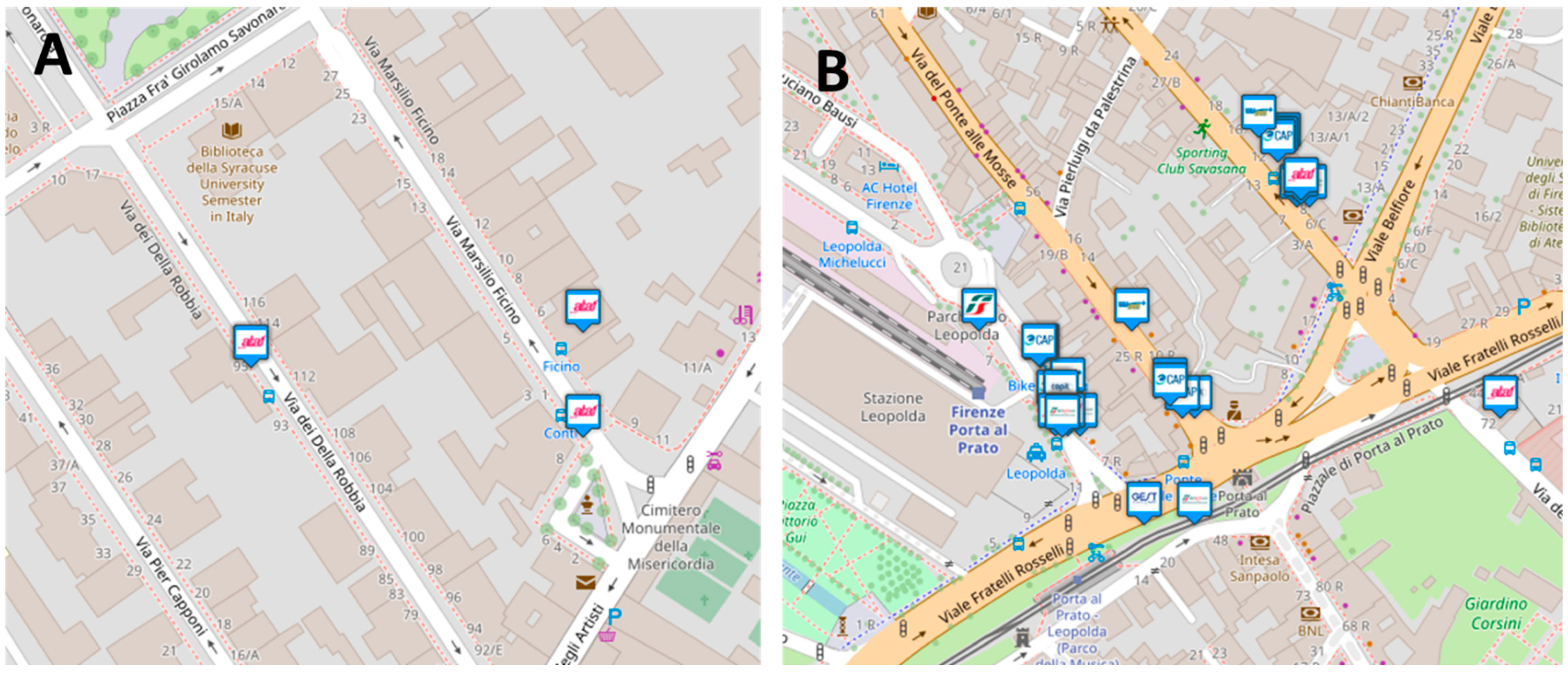
• Multi-operativity: It manages the offers of different mobility operators. In the city of Florence, we have 13 main mobility operators (e.g., ATAF, Trenitalia, GEST, etc.). The distribution of their services is not uniform.
• changing the offer and the demand in the scenarios of analysis by creating new scenarios, changing the offer and also the services in the maps, and knowledgebase. More details are reported in Section 6.
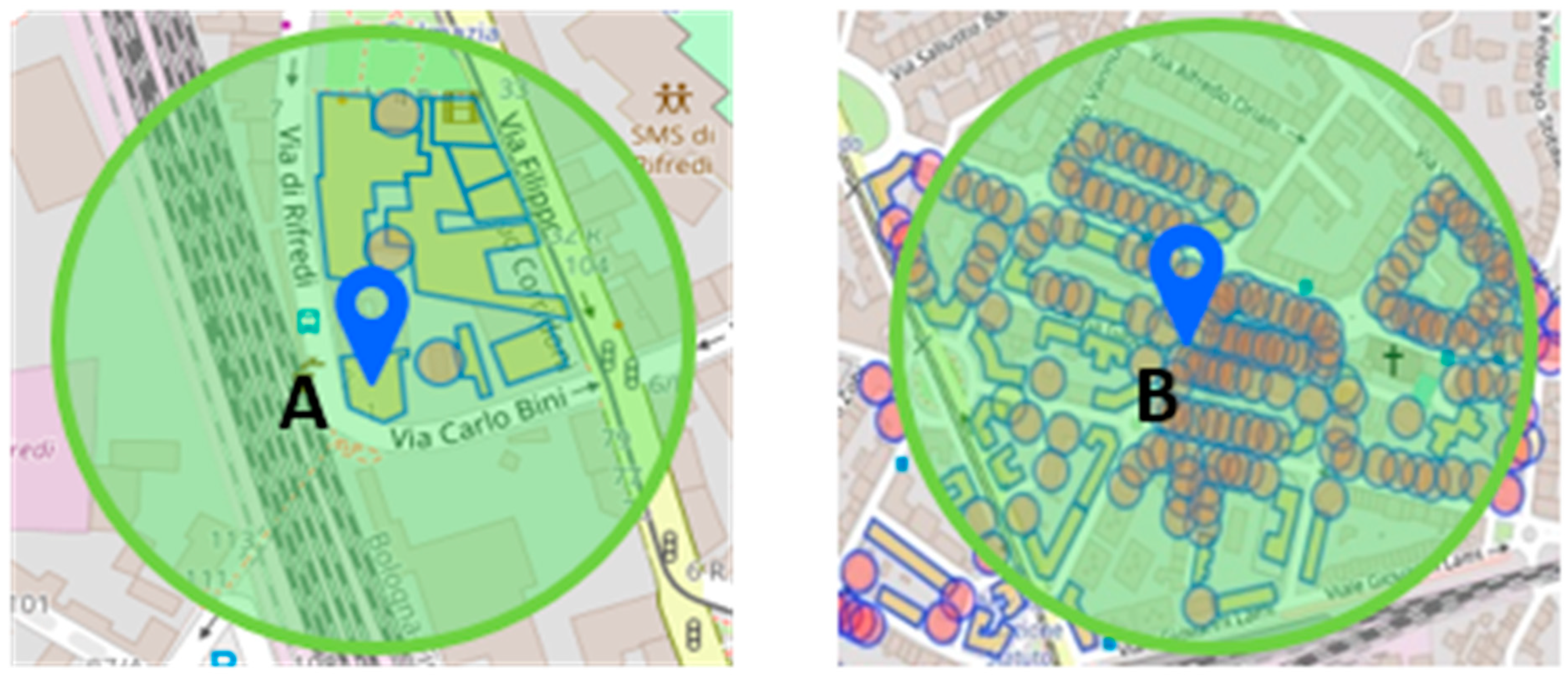
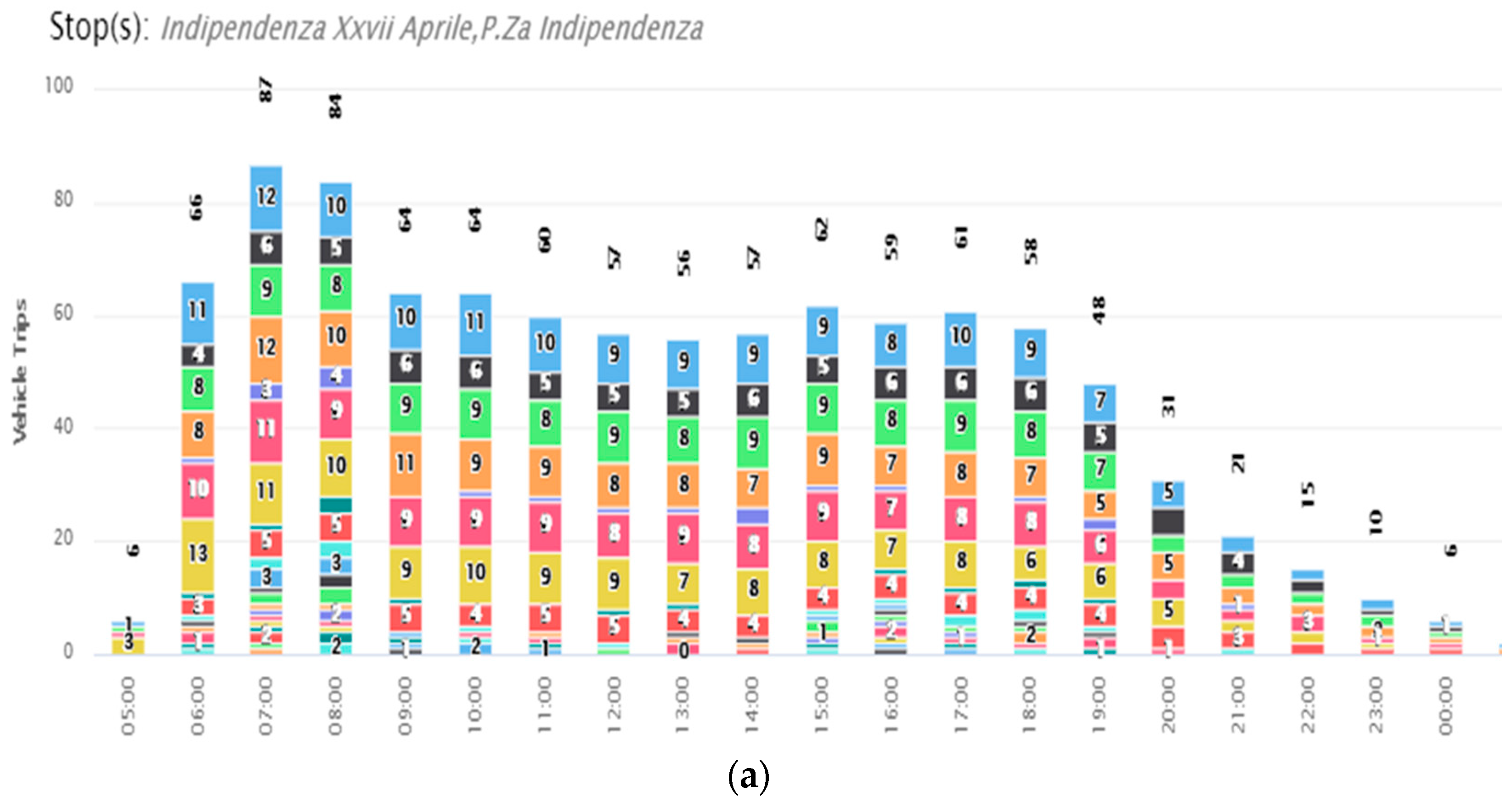
• computing KPIs and related evidence information to perform the PTS analysis and provide support for decision makers about mobility policies in the city. The most relevant KPIs include the number pick-ups and drop-offs at a given stop over time. Moreover, nearby POIs (shopping centers, offices, shops, tourist attractions) along with each vehicle line, the number of vehicle lines and trips in each time interval are the examples of provided information to support the scenario analysis.
• exploiting a range of data sources, from the rich Km4City knowledge base [41,42,44] which leads to a more robust computational model, more complete scenario.

On the DORAM home page (see Figure 9), the Stop panel on the right reports the analysis of the bus stops. It presents the most crowded stops in the city in decreasing order of the sum of daily pick-ups and drop-offs. For each stop in the Stop panel, mobility operator(s) that provide services are shown. Moreover, it is possible to search for stops by text and by clicking in an area. On the bottom, general information regarding the service offer (e.g., # of stops, mobility operators) and the mobility demand (e.g., daily commuter trips, residential buildings) are reported.

DORAM also provides KPIs support the decision maker/user to understand in which extent the demand is met by the offer, (see Figure 10) in terms of pick-ups and drop-offs over time. In addition, it is possible to analyze KPIs in different time intervals defined by the user, using the combo boxes on the top of the Stop panel (see Figure 9).

Evidence information, it is used to support KPIs for each stop. To mention a few; (1) total daily drop-offs, pick-ups and vehicle trips, in the Stop panel (see Figure 9), (2) drop-offs, pick-ups, and vehicle trips, (for instance, see Figure 11a) for each line in each time interval, by clicking on Daily Drop-offs, Daily Pick-ups, and Daily Vehicle Trips in the Stop panel, (3) line information, by clicking on the line direction (see Figure 11b), (4) nearby services (e.g., offices, stores), by clicking on Services on the route button (see Figure 11c), passing vehicle lines and their directions.

6. Scenarios Analysis and Results

In this section, we discuss the evaluation of Actual Scenario together with the analysis of a sample defined alternative scenario.

6.1. Validation of the DORAM Model and Weights

ATAF has performed a campaign of measures on a wide number of bus stops and vehicles to count the number of people over time, in several days of the week, and lines. Focusing on the city of Florence, we used the ATAF dataset, splitting the data in those used to tune the model and to assess the results of the DORAM model for Actual Scenario. In order to validate DORAM model, we compared the data produced by the model with respect to those measured by ATAF.

Table 3. ATAF dataset description.

Feature	ATAF Dataset	Florence (Total)
Service time span	$05:00 \mathrm{to} 01:59$ (next day)	$04:00 \mathrm{to} 01:59$(next day)
Lines	$25$ (21.92%)	$114$
Trips	1173 (16.67%)	$7033$
Stops	$942 \left(62.26\%\right)$	1513

describes the ATAF dataset.

Table 4. Simulation setup for Actual Scenario.

Parameter	Value
Morning time	$05:00-13:59$
Afternoon time	$14:00-01:59$ (next day)
Time interval size	$59 \left(\min \right)$
Radius r around stop s	$200 \left(\mathrm{m}\right)$
$\mathrm{Total} \left(\mathrm{morning}\right) \mathrm{pick}\text{-}\mathrm{ups} pck\left(mng\right)$	83,125
$\mathrm{Total} \left(\mathrm{afternoon}\right) \mathrm{drop}\text{-}\mathrm{offs} pck\left(aft\right)$	75,234

reports the simulation setup when analyzing Actual Scenario.

The evaluation of results is reported in

Table 5. The values of features in ATAF dataset in the city of Florence.

		Pick-Ups	Drop-Offs
Whole ATAF dataset	Max.	59	59
	Avg.	1.27	1.27
	RMSE	2.74	2.74
	MAE	$1.36$	1.44
	MASE	0.89	0.94
	MSE	−0.8	−0.7
Removing 1% of outliers in ATAF dataset	Max.	10	10
	Avg.	1.09	1.09
	RMSE	1.98	2.05
	MAE	1.17	1.25
	MASE	0.91	0.97
	MSE	−0.6	−0.5

. We used RMSE (Root-Mean-Square Deviation), MAE (Mean Absolute Error) and MASE (Mean Absolute Scaled Error) which are the most known performance metrics.

The results put in evidence limited errors, and they have been confirmed acceptable by city operators and decision makers.

6.2. Alternative Scenario Analysis

In order to make a decision multiple scenarios can be produced, and it is possible to analyze the impact of changes with respect to a reference scenario (e.g., the actual). Thus, to create a new scenario, the data of the mobility demand and the service offer are loaded in a new instance of the knowledge base. To this end, it is possible to use GTFS management tools (e.g., static GTFS manager) to generate (or update) the service offer and mobility demand (e.g., changing the number of trips or vehicle lines passing a stop, adding a stop, changing the location of a stop).

For example, Indipendenza XXVII Aprile stop, operated by ATAF, which is called p.Za Indipendenza by another mobility operator (Busitalia), is the most crowded stop in the city of Florence with for each day more than $377$ pick-ups and $407$ drop-offs, in accordance with the DORAM model. It indicates that, a considerable number of people wait at the stop during a working day. Such a situation could cause several consequences (e.g., high passenger destiny at the stop, increasing waiting time at the stop, decreasing operating speed, decreasing travel time reliability [46]). The solution has been to balance the number of waiting people at crowded stops and, to mitigate the problem, we created a scenario with a modified offer, called Alternative Scenario splitting the lines by (see Figure 1): (1) adding an alternative stop, (e.g., called Cosimo Ridolfi), in a suitable location (e.g., Indipendenza XXVII Aprile) stop; (2) transferring some line(s) to the newly added stop. For the sake of clearness, the mentioned bus-stop Indipendenza XXVII Aprile is located in the central area of Florence, and it represents a fundamental and crowded stop in the city. In the case, the alternative scenario with respect to the actual one is related to a new bus-stop creation near the bus-stop Indipendenza XXVII Aprile, for example in the nearest road which is called Cosimo Ridolfi. Then, a new bus stop called Cosimo Ridolfi is considered which is hypothetical bus stop located about 200 m away from the bus stop called Indipendenza XXVII Aprile, so that, some lines which pass through the bus stop Indipendenza XXVII Aprile could be transferred in the newly created bus stop Cosimo Ridolfi. By applying the DORAM tool in the context of what-if analysis to such a case, lines 1 and 23, which are the two of the most frequent lines among those that pass through Indipendenza XXVII Aprile stop, have been transferred to the new stop Cosimo Ridolfi. As a result, the commuters have been constrained to move at the new stop for commuting, and consequently, the number of waiting commuters to be picked-up and those who are dropped-off at Indipendenza XXVII Aprile stop will be decreased.

Table 6. The comparison of Actual Scenario and Alternative Scenario.

Scenario	ActualScen.		Alternative Scenario
Stop	Indipendenza XXVII Aprile		Indipendenza XXVII Aprile		Cosimo Ridolfi
Mobility Operator	ATAF	Busitalia	ATAF	Busitalia	ATAF	Busitalia
Lines	$9$	$20$	$27$	$20$	$2$	-
Daily pick-ups	$377$		$334$$(-11.4\%$ compared to Actual Scenario)		$65$
Daily drop-offs	$407$		$362$$(-11.05\%$ compared to Actual Scenario)		$75$

shows a comparison between Actual Scenario and Alternative Scenario. As one can see, in Alternative Scenario, daily pick-ups and drop-offs are respectively decreased by $-11.4\%$ and $-11.05\%$ at Indipendenza XXVII Aprile stop, compared to in Actual Scenario. Therefore, defining Alternative Scenario can suitably distribute waiting people among Indipendenza XXVII Aprile and Cosimo Ridolfi stops.

7. Conclusions

A model and tool, called DORAM, has been introduced in this paper. It allows to perform the analysis of public transportations offer with respect to the demand (taking into account a set of possible data sources), in a multi-modal and multi-operator context. More precisely, the formal mathematical model related to DORAM has been introduced, in order to analyze the mobility demand with respect to the public transport offer taking into account a range of contextual and operative data. The DORAM solution investigates how the demand is satisfied in terms of public transportation mobility by means of simulation tools and KPIs and the related evidence information with the aim of identifying crowded conditions on bus-stops and on the busses, that influence the experience of transportation.

In the present work, we first analyzed the current status of a public transportation system by matching the service offer, in terms of public transportation means, and the mobility demand. This allowed us to tune the model and identify the parameters that express the relationship of the mobility demand with the city context and census data. Then, we focused on creating alternative scenarios, where a set of changes are introduced in the current status of a public transportation system and comparing the available scenarios by quickly switching between them, with the aim of reducing the crowded conditions on busses and at bus-stops. While the computational model of DORAM is enriched by the usage of a wide range of data sources, investigating public transportation systems in DORAM is equipped with computing relevant KPIs (e.g., pickups and drop-offs at a stop) and related evidence information (e.g., the number of passing trips and lines, considering a stop). DORAM can suitably be used by urban decision-makers and mobility when deciding on a (set of) plans to improve the public transportation networks, especially in the presence of critical situations (e.g., overcrowded or blocking stops, overcrowded vehicles). DORAM model and solution has been validated on the basis of data collected on the field by major public transportation companies in the Florence Area, that are: ATAF and BUSITALIA. The DORAM tool demonstrated to be capable to identify critical problems without the needs of investing large amount of money for physical campaign of data collection. Moreover, DORAM solution performs what-if analysis by analyzing the impact of a (set of) change(s) of the Actual Scenario to see their effects in terms of people flows and matching demand/offer. Then, DORAM provides non-functional features such as (i) flexibility, by taking into account different data sources, (ii) fast-computability, quickly switch between different scenarios, and (iii) web-based interface that supports GTFS data and REST APIs for analysis results.

DORAM is presently accessible from: https://www.snap4city.org/odanalyzer/#b (accessed on 5 September 2022) and with more functionalities if you perform free registration on Snap4City.org.

References

1. Afrin, T.; Yodo, N. A Survey of Road Traffic Congestion Measures towards a Sustainable and Resilient Transportation System. Sustainability 2020, 12, 4660. [Google Scholar] [CrossRef]
2. Bilotta, S.; Nesi, P. Traffic flow reconstruction by solving indeterminacy on traffic distribution at junctions. Future Gener. Comp. Syst. 2021, 114, 649–660. [Google Scholar] [CrossRef]
3. Bellini, P.; Bilotta, S.; Nesi, P.; Paolucci, M.; Soderi, M. Real-Time Traffic Estimation of Unmonitored Roads. In Proceedings of the 2018 IEEE 16th Intl Conf on Dependable, Autonomic and Secure Computing, 16th Intl Conf on Pervasive Intelligence and Computing, 4th Intl Conf on Big Data Intelligence and Computing and Cyber Science and Technology Congress(DASC/PiCom/DataCom/CyberSciTech), Athens, Greece, 12–15 August 2018; pp. 935–942. [Google Scholar] [CrossRef]
4. Smit, R.; Ntziachristos, L.; Boulter, P. Validation of road vehicle and traffic emission models—A review and meta-analysis. Atmos. Environ. 2010, 44, 2943–2953. [Google Scholar] [CrossRef]
5. Bilotta, S.; Nesi, P. Estimating CO2 Emissions from IoT Traffic Flow Sensors and Reconstruction. Sensors 2022, 22, 3382. [Google Scholar] [CrossRef] [PubMed]
6. Kathuria, A.; Parida, M.; Sekhar, C.R. A Review of Service Reliability Measures for Public Transportation Systems. Int. J. Intell. Transp. Syst. Res. 2020, 18, 243–255. [Google Scholar] [CrossRef]
7. Chang, J.S. Assessing travel time reliability in transport appraisal. J. Transp. Geogr. 2010, 18, 419–425. [Google Scholar] [CrossRef]
8. Agarwal, S.; Diao, M.; Keppo, J.; Sing, T.F. Preferences of public transit commuters: Evidence from smart card data in Singapore. J. Urban Econ. 2020, 120, 103288. [Google Scholar] [CrossRef]
9. Static GTFS Manager. Available online: https://static-gtfs-manager.herokuapp.com/ (accessed on 16 October 2020).
10. Antunes, H.; Figueiras, P.; Costa, R.; Teixeira, J.; Jardim, R. Analysing Public Transport data through the use of Big Data technologies for urban mobility. In Proceedings of the 2019 International Young Engineers Forum (YEF-ECE), Hong Kong, 27 April 2019; pp. 40–45. [Google Scholar] [CrossRef]
11. Widyawan, B.; Putra, D.W.; Kusumawardani, S.S.; Widhiyanto, B.T.Y.; Habibie, F. Big data analytic for estimation of origin-destination matrix in Bus Rapid Transit system. In Proceedings of the 2017 3rd International Conference on Science and Technology—Computer (ICST), Dubai, United Arab Emirates, 27–28 May 2017; pp. 165–170. [Google Scholar] [CrossRef]
12. Tanaka, M.T.; Kimata, T.; Arai, T. Estimation of Passenger Origin-Destination Matrices and Efficiency Evaluation of Public Transportation. In Proceedings of the 2016 5th IIAI International Congress on Advanced Applied Informatics (IIAI-AAI), Kumamoto, Japan, 10–14 July 2016; pp. 1146–1150. [Google Scholar] [CrossRef]
13. Zapata, L.P.; Flores, M.; Larios, V.; Maciel, R.; Antunez, E.A. Estimation of people flow in public transportation network through the origin-destination problem for the South-Eastern corridor of Quito city in the smart cities context. In Proceedings of the 2019 IEEE International Smart Cities Conference (ISC2), Casablanca, Morocco, 14–17 October 2019; pp. 181–186. [Google Scholar] [CrossRef]
14. Abou-Zeid, M.; Fujii, S. Travel satisfaction effects of changes in public transport usage. Transportation 2016, 43, 301–314. [Google Scholar] [CrossRef]
15. Van Oort, N.; Brands, T.; de Romph, E. Short term ridership prediction in public transport by processing smart card data. Transp. Res. Rec. 2015, 2535, 105–111. [Google Scholar] [CrossRef]
16. Lam, A.Y.S. Combinatorial Auction-Based Pricing for Multi-Tenant Autonomous Vehicle Public Transportation System. IEEE Trans. Intell. Transp. Syst. 2016, 17, 859–869. [Google Scholar] [CrossRef]
17. Shang, S.; Guo, D.; Liu, J.; Liu, K. Human Mobility Prediction and Unobstructed Route Planning in Public Transport Networks. In Proceedings of the 2014 IEEE 15th International Conference on Mobile Data Management, Brisbane, Australia, 15–18 July 2014; Volume 2, pp. 43–48. [Google Scholar] [CrossRef]
18. Sun, L.; Tirachini, A.; Axhausen, K.W.; Erath, A.; Lee, D.H. Models of bus boarding and alighting dynamics. Transp. Res. Part A Policy Pract. 2014, 69, 447–460. [Google Scholar] [CrossRef]
19. Arnone, M.; Delmastro, T.; Giacosa, G.; Paoletti, M.; Villata, P. The Potential of E-ticketing for Public Transport Planning: The Piedmont Region Case Study. Transp. Res. Procedia 2016, 18, 3–10. [Google Scholar] [CrossRef]
20. Zhang, J.; Shen, D.; Tu, L.; Zhang, F.; Xu, C.; Wang, Y.; Li, Z. A Real-Time Passenger Flow Estimation and Prediction Method for Urban Bus Transit Systems. IEEE Trans. Intell. Transp. Syst. 2017, 18, 3168–3178. [Google Scholar] [CrossRef]
21. Cao, Z.; Ceder, A.; Zhang, S. Real-time schedule adjustments for autonomous public transport vehicles. Transp. Res. C Emer. 2019, 109, 60–78. [Google Scholar] [CrossRef]
22. Oviedo, D.; Granada, I.; Perez-Jaramillo, D. Ridesourcing and Travel Demand: Potential Effects of Transportation Network Companies in Bogotá. Sustainability 2020, 12, 1732. [Google Scholar] [CrossRef]
23. Niu, H.; Zhou, X. Optimizing urban rail timetable under time-dependent demand and oversaturated conditions. Transp. Res. C Emer. 2013, 36, 212–230. [Google Scholar] [CrossRef]
24. Liu, T.; Ceder, A. Analysis of a new public-transport-service concept: Customized bus in China. Transp. Policy 2015, 39, 63–76. [Google Scholar] [CrossRef]
25. Liu, R.; Li, S.; Yang, L.; Yin, J. Energy-Efficient Subway Train Scheduling Design with Time-Dependent Demand Based on an Approximate Dynamic Programming Approach. IEEE T. Syst. Man Cy-S 2020, 50, 2475–2490. [Google Scholar] [CrossRef]
26. Seaborn, C.; Attanucci, J.; Wilson, N.H.M. Analyzing Multimodal Public Transport Journeys in London with Smart Card Fare Payment Data. Transp. Res. Rec. 2009, 2121, 55–62. [Google Scholar] [CrossRef]
27. Castellanos, J.C.; Fruett, F. Embedded system to evaluate the passenger comfort in public transportation based on dynamical vehicle behavior with user’s feedback. Measurement 2014, 47, 442–451. [Google Scholar] [CrossRef]
28. Wu, W.; Zheng, Y.; Cao, N.; Zeng, H.; Ni, B.; Qu, H.; Ni, L.M. MobiSeg: Interactive region segmentation using heterogeneous mobility data. In Proceedings of the 2017 IEEE Pacific Visualization Symposium (PacificVis), Seoul, Korea, 18–21 April 2017; pp. 91–100. [Google Scholar] [CrossRef]
29. Li, Z.; Hensher, D.A. Performance contributors of bus rapid transit systems: An ordered choice approach. Econ. Anal. Policy vol. 2020, 67, 154–161. [Google Scholar] [CrossRef]
30. Horni, A.; Nagel, K.; Axhausen, K.W. The Multi-Agent Transport Simulation MATSim; Ubiquity Press London: London, UK, 2016. [Google Scholar]
31. Krajzewicz, D.; Erdmann, J.; Behrisch, M.; Bieker, L. Recent Development and Applications of SUMO—Simulation of Urban Mobility. Int. J. Adv. Syst. Meas. 2012, 3, 128–138. [Google Scholar]
32. Smith, L.; Beckman, R.; Baggerly, K. TRANSIMS: Transportation Analysis and Simulation System; Los Alamos National Laboratory: Santa Fe, NM, USA, 1995. [Google Scholar]
33. Di Lorenzo, G.; Sbodio, M.L.; Calabrese, F.; Berlingerio, M.; Nair, R.; Pinelli, F. Allaboard: Visual exploration of cellphone mobility data to optimise public transport. IEEE TVCG 2016, 22, 1036–1050. [Google Scholar] [CrossRef]
34. MOSAiC Project: Mobility 4.0 for Smart Cities. Available online: https://www.disit.org/drupal/?q=node/7174 (accessed on 5 September 2022).
35. Bellini, P.; Benigni, M.; Billero, R.; Nesi, P.; Rauch, N. Km4City ontology building vs. data harvesting and cleaning for smart-city services. J. Vis. Lang. Comput. 2014, 25, 827–839. [Google Scholar] [CrossRef] [Green Version]
36. Badii, C.; Bellini, P.; Difino, A.; Nesi, P. Smart City IoT Platform Respecting GDPR Privacy and Security Aspects. IEEE Access 2020, 8, 23601–23623. [Google Scholar] [CrossRef]
37. Bellini, E.; Bellini, P.; Cenni, D.; Nesi, P.; Pantaleo, G.; Paoli, I.; Paolucci, M. An IoE and Big Multimedia Data Approach for Urban Transport System Resilience Management in Smart Cities. Sensors 2021, 21, s21020435. [Google Scholar] [CrossRef]
38. Bellini, P.; Cenni, D.; Nesi, P.; Paoli, I. Wi-Fi based city users’ behaviour analysis for smart city. J. Vis. Lang. Comput. 2017, 42, 31–45. [Google Scholar] [CrossRef]
39. Sohn, K.; Kim, D. Dynamic Origin-Destination Flow Estimation Using Cellular Communication System. IEEE Trans. Veh. Technol. 2008, 57, 2703–2713. [Google Scholar] [CrossRef]
40. OpenStreetMap. Available online: www.openstreetmap.org (accessed on 1 April 2019).
41. Istituto Nazionale di Statistica. Available online: https://www.istat.it/en/ (accessed on 5 September 2022).
42. The Region Tuscany Digital Portal. Available online: http://www.regione.toscana.it/ (accessed on 5 September 2022).
43. ServiceMap. Available online: http://servicemap.disit.org/ (accessed on 5 September 2022).
44. Nesi, P.; Badii, C.; Bellini, P.; Cenni, D.; Martelli, G.; Paolucci, M. Km4City Smart City API: An Integrated Support for Mobility Services. In Proceedings of the 2016 IEEE International Conference on Smart Computing (SMARTCOMP), St. Louis, MO, USA, 18–20 May 2016; pp. 1–8. [Google Scholar] [CrossRef]
45. Overpass Turbo Tool. Available online: http://overpass-turbo.eu/ (accessed on 5 September 2022).
46. Tirachini, A.; Hensher, D.A.; Rose, J.M. Crowding in public transport systems: Effects on users, operation and implications for the estimation of demand. Transp. Res. Part A Policy Pract. 2013, 53, 36–52. [Google Scholar] [CrossRef]
Figure 1. The general DORAM architecture.
Applsci 12 08982 g001
Figure 2. W2H and H2W trips.
Applsci 12 08982 g002
Figure 3. Using public transport systems by the commuters with private vehicles who work or study in the restricted traffic zones.
Applsci 12 08982 g003
Figure 4. In the left, an example of single-stage trip having a beginning s b e g and final s f i n stop. In the right, an example of multi-stage trip having transfer stops s t r a also.
Applsci 12 08982 g004
Figure 5. Density of stops near two sample stops A and B.
Applsci 12 08982 g005
Figure 6. Density of residential buildings around stops A and B.
Applsci 12 08982 g006
Figure 7. Density of services around stops A and B.
Applsci 12 08982 g007
Figure 8. Morning W m n g and afternoon W a f t weight vectors examples.
Applsci 12 08982 g008
Figure 9. DORAM homepage.
Applsci 12 08982 g009aApplsci 12 08982 g009b
Figure 10. An example of the DORAM KPIs (pick-ups and drop-offs in each time interval) for a stop.
Applsci 12 08982 g010
Figure 11. Examples of evidence information: (a) pick-ups, drop-offs, and vehicle trips, (b) Line information, (c) Line nearby services.
Applsci 12 08982 g011aApplsci 12 08982 g011b