An Improved Method Based on EEMD-LSTM to Predict Missing Measured Data of Structural Sensors

Abstract

Time history testing using a shaking table is one of the most widely used methods for assessing the dynamic response of structures. In shaking-table experiments and on-site monitoring, acceleration sensors are facing problems of missing data due to the fact of measurement point failures, affecting the validity and accuracy of assessing the structural dynamic response. The original measured signals are decomposed by ensemble empirical mode decomposition (EEMD), and the widely used deep neural networks (DNNs), gated recurrent units (GRUs), and long short-term memory networks (LSTMs) are used to predict the subseries of the decomposed original measured signal data to help model and recover the irregular, periodic variations in the measured signal data. The raw acceleration data of a liquefied natural gas (LNG) storage tank in shaking-table experiments were used as an example to compare and discuss the method’s performance for the complementation of missing measured signal data. The results of the measured signal data recovery showed that the hybrid method (EEMD based) proposed in this paper had a higher complementary performance compared with the traditional deep learning methods, while the EEMD-LSTM exhibited the best missing data complementary accuracy among all models. In addition, the effect of the number of prediction steps on the prediction accuracy of the EEMD-LSTM model is also discussed. This study not only provides a method to fuse EEMD and deep learning models to predict measured signal’ missing data but also provides suggestions for the use of EEMD-LSTM models under different conditions.

1. Introduction

In recent years, earthquake disasters have frequently occurred, causing severe casualties and economic losses in many countries [1]. The emergency response after an earthquake is essential for saving lives; thus, a large number of studies have focused on the impact of earthquakes on structures. In order to accurately estimate the damage to building structures from earthquakes of different intensities, the dynamic response of structures under earthquake action needs to be studied.

Shaking-table experimental technology can be used to test the response of structures and soil to verify their seismic performance. It is a device used to shake scaled structural models with various simulated ground motions. Time history testing using a shaking table is one of the most widely used methods to evaluate the dynamic response of structures [2]. Currently, a large number of dynamic studies using a shaking table can be found in the academic literature. For example, Betti et al. [3] conducted a prototype two-story masonry building on a shaking table at the CNR-ENEA Research Center in Italy. They analyzed the behavior of the prototype from initial elasticity to the large-scale destruction of development. Wang et al. [4] tested a full-scale model of a recycled aggregate block masonry building on a shaking table. The intrinsic frequency, equivalent stiffness, structural damping ratio, acceleration response, seismic force response, displacement response, and structural brittleness were discussed. Lignos et al. [5] conducted full-scale high-rise building shaking-table tests and demonstrated the validity of the numerical model used. Based on these parameters and test results, researchers were able to explain the dynamic behavior of the structure.

Shaking-table tests are an important and effective method to study earthquake engineering, and they can obtain the response of a structure under a specific seismic excitation. A large number of sensors need to be arranged in the tests to record the acceleration response and displacement response of the structure. However, in shaking table tests, the sensors face the problem of missing data due to the failure of the measurement points. This means that the recorded test data do not fully reflect the structure’s actual dynamic response, negatively impacting the later structural response analysis. Therefore, it is worthwhile to investigate how to complement the response of the remaining test period based on the recorded partial response data.

In recent years, deep learning techniques, such as deep neural networks (DNNs), long short-term memory neural networks (LSTMs), and gated recurrent units (GRUs), have shown great potential in establishing nonlinear mapping rules between complex patterns in time series. Recurrent neural networks (RNNs) are specifically designed to learn continuous, time-varying, and linear/nonlinear patterns for regression problems [6,7]. LSTM [8] is an improved version of recurrent neural network (RNN) architecture. It has been shown to be an appropriate tool over long time windows to identify various features of the input time history, and it has been applied to applications such as sequence labeling [9], natural language processing [10], and automatic driving [11].

Before this, much research was conducted to develop critical features for capturing time series data using deep learning models. For example, Panakkat et al. [12] used recurrent neural network modeling with eight indicators of seismic activity as input to predict the time and location of earthquakes. Kuyuk and Park et al. [13,14] proposed a recurrent neural network framework that can be used to classify seismic waveforms. The model achieved good results in the seismic signal classification task. Bhandarkar et al. [15] used a long short-term memory neural network to model earthquake sequences, and the trained model can be used to predict future trends in earthquakes. The results were compared with ordinary feedforward neural network solutions, showing that the LSTM neural network had better performance. Zhang et al. [16] developed an LSTM model for predicting building response based on ground motion records and structural properties. It was shown that the LSTM network was a reliable and computationally efficient method for predicting nonlinear structural response. Perez-Ramirez et al. [17] combined recurrent neural networks with Bayesian training for the response prediction of large buildings. The proposed method exhibited excellent results in actual conditions, with the advantage of low computational cost. Kim et al. [18] proposed an adaptive algorithm that identifies the optimal number and location of sensors within a given urban area and uses deep neural networks to estimate regional structural damage given a spatial distribution of earthquake intensity levels. Lu et al. [19] generated time–frequency distribution maps of ground shaking as a detailed visual representation of the frequency domain features and time-domain features of ground shaking. These data were then used to train convolutional neural network CNN models, which could predict damage states effectively.

Research on hybrid models with deep learning methods to complement missing data has gradually increased. Liu et al. [20] combined empirical modal decomposition with a long and short-term memory deep learning network to recover the measured signal data. This hybrid model transformed the missing data prediction work into a time series prediction work, which was then solved using a partitioning strategy. Chen et al. [21] proposed a baseline correction method based on EMD-DNN, which used deep neural networks (DNNs) to extract features from the multiple time series obtained by EMD based on removing the drifting trend with empirical modal decomposition (EMD) and, finally, achieved the prediction of the actual displacement. Liu et al. [20] proposed an EMD-BiGRU model for missing data prediction. The proposed model could better capture the microscopic changes in the measured data and exhibited better prediction performance than the pure machine learning algorithm. However, there are two problems in using EMD to decompose the measured signal data: first, the IMF obtained by decomposition with EMD suffers from modal mixing, which results in inaccurate IMF components; second, the end effect affects the decomposition effect. Wu et al. [22] proposed an improved EMD method based on a noise-assisted analysis called ensemble empirical mode decomposition (EEMD), using EMD to analyze the results after white noise decomposition. EEMD can effectively suppress the modal mixing phenomenon of EMD and has a better decomposition effect.

From the above studies, it is clear that deep learning methods (i.e., DNN, GRU, and LSTM) have attracted the attention of many researchers and have been widely used in the field of earthquake engineering. These previous studies confirm the utility and success of employing RNN (or LSTM) to capture various ground motion features and approximate the response of various building types. A common implication of all these prior studies is that alternative models can establish an accurate mapping between the recorded time-history data and the structural response. The goal of forming mappings between complex patterns of sensor time series and missing response data follows similar thinking. However, few models have been used to address the under-recorded sensor data in earthquake engineering. In addition, although shaking-table tests are used as an effective method to obtain the acceleration and displacement responses of structures under seismic excitation, they also face the problem of missing data due to the failure of sensors, which has an impact on structural response analysis. Given the ability of EEMD to decompose the measured signal data and the powerful performance of deep learning methods in time series prediction tasks, this study not only provides a method to predict the missing data of measured signals by EEMD-based models incorporating deep learning but also provides suggestions for EEMD-LSTM models to be used for different conditions.

In Section 2, the principles of the used method are described more concretely, and the relevant details of the experiments are provided in Section 3. In Section 4, the experiments and prediction results are provided for analysis. Finally, in Section 5, the conclusions regarding the different models are given.

2. Theoretical Background of the Models

2.1. Ensemble Empirical Mode Decomposition

EEMD (ensemble empirical mode decomposition) is one of the most common EMD improved methods, and its advantage is that it can solve the modal blending phenomenon in EMD methods. The mode overlap phenomenon (i.e., the signals of different modes are mixed), generally has two cases: one is that the signals of different feature scales appear in one IMF component; the other is that the signals of the same feature scale are dispersed into different IMF components. The article’s detailed methodology of the EMD method can be found in [23].

The main improved idea of EEMD is to use the property that the mean value of the white noise is 0. By introducing uniformly distributed white noise several times in the decomposition process, the noise in the signal is masked by the noise added artificially several times to obtain more accurate upper and lower envelopes. At the same time, the decomposition results are averaged, and the more times the averaging process is performed, the less the noise is brought into the decomposition.

The main steps in EEMD decomposition can be found in Figure 1.

(1).

Setting the original signals’ processing times to be equal, m;

(2).

Adding random white noise of different amplitudes to each of these m original signals to form a new series of signals;

(3).

Performing EMD decomposition on each of these new signals to obtain a series of IMF components;

(4).

The EEMD decomposition results are obtained by averaging the IMF components of the corresponding modes separately.

EEMD can decompose the original signal data into a linear combination of a finite number of intrinsic mode functions (IMFs), with high to low frequencies, and each IMF component of the decomposition contains local feature signals of the original signal at different time scales. Therefore, the EEMD algorithm can be used to decompose more time-dimensional features of the original signal data. The decomposed time-dimensional features are input into the LSTM network model to extract time-dimensional features to predict the missing parts of the original signal data. Among them, the decomposed IMFs do not need to satisfy other conditions to be input into the subsequent LSTM network model.

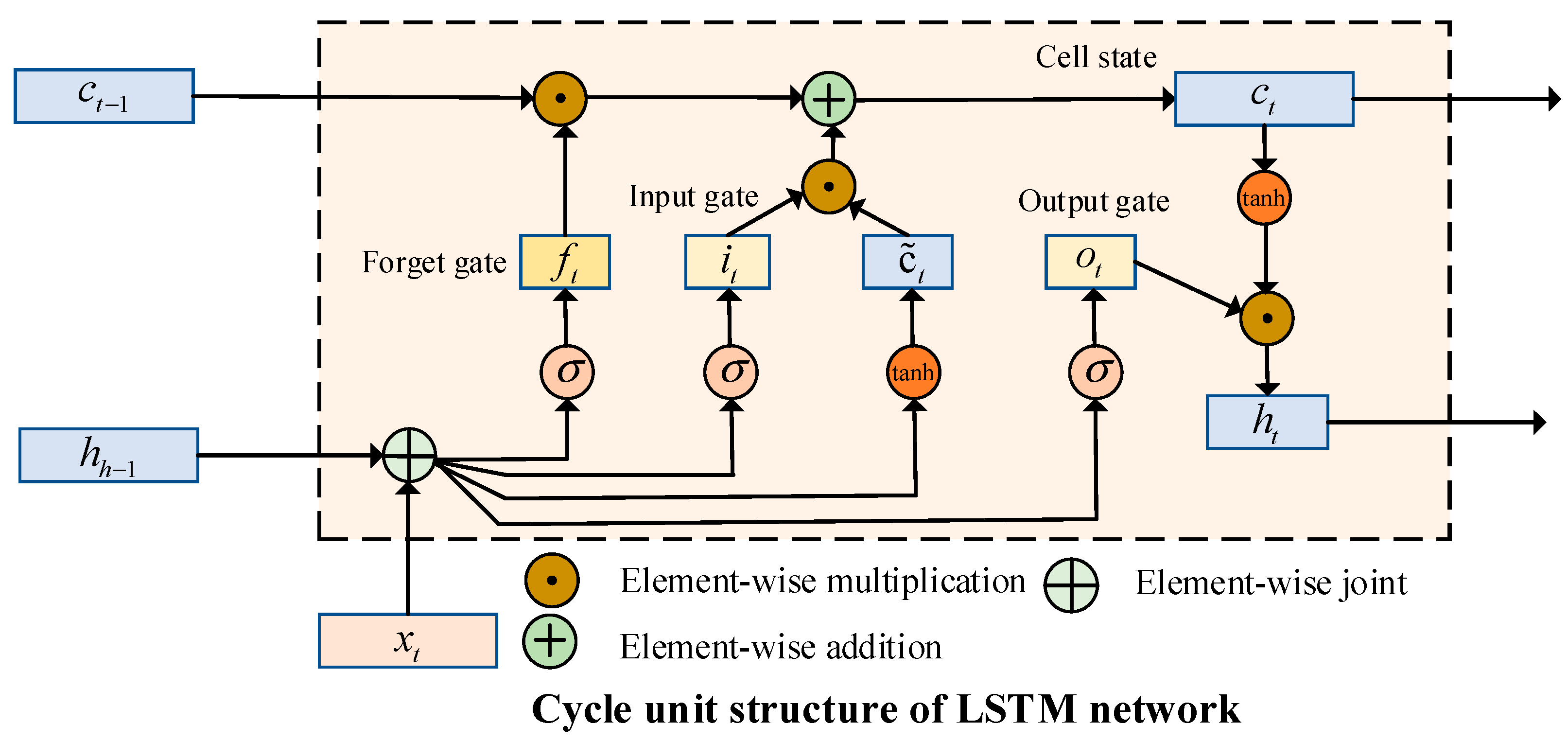
2.2. Long Short-Term Memory

As a variant of recurrent neural networks, proposed by Hochreiter [8], it has been widely used in time series prediction problems. With the advantage of mapping all historical data to each prediction and, thus, remembering the long-term temporal correlation of time series, LSTM has made fantastic progress in the field of time series such as speech recognition.

The difference between an RNN and DNN is the connection between the hidden layers. The hidden state of the previous time step in an RNN can be used as input for the current time step so that features can be transferred forward or backward. The main component of the LSTM network is the memory block, which introduces a memory mechanism based on RNN, i.e., by providing three special adaptive multiplicative gates to decide whether to retain or remove temporal information.

As can be seen from Figure 2, three gate units—an input gate, output gate, and forget gate—were used in the LSTM unit to control the information transfer. Usually, the time series data of each time step and the previous hidden state are used as the input for the LSTM unit. The input gate, $i_t$, can control the current moment of the candidate status, ${\tilde{c}}_t$, which needs to save the information; the forget gate, $f_t$, can control the internal state, $c_{t-1}$, of the last moment, which needs to discard information; the output gate, $o_t$, can control the internal state’s, $c_t$, output information to the external state, $h_t$, at the current moment.

The computational process inside the cyclic cell structure in an LSTM network is as follows:

First, calculate the input gate, the output gate, the forget gate, and the candidate state using the external state at the last moment, $h_{t-1}$, and the current moment, $x_t$.

Second, update the memory cell, $c_t$, by combining the forget gate, $f_t$, and the input gate, $i_t$.

Finally, combine the output gate, $o_t$, to transfer the internal state information to the external state, $h_t$.

The LSTM will accumulate important feature information for the final prediction results during the processing of the time series data and make full use of the historical data through the back propagation process, corresponding to the LSTM update equation as follows:

$$i_t=\sigma (W_i{x}_t+U_i{h}_{t-1}+b_i)$$

(1)

$$f_t=\sigma (W_f{x}_t+U_f{h}_{t-1}+b_f)$$

(2)

$$o_t=\sigma (W_o{x}_t+U_o{h}_{t-1}+b_o)$$

(3)

$$c_t=f_t\odot c_{t-1}+i_t\odot {\tilde{c}}_t$$

(4)

$$h_t=o_t\odot \tanh (c_t)$$

(5)

$${\tilde{c}}_t=\tanh (W_c{x}_t+U_c{h}_{t-1}+b_c)$$

(6)

where $x_t$ is the input vector at moment $t$; $i_t$, $o_t$, $f_t$, and $\sigma$ are the input gate, output gate, forget gate, and sigmoid function, respectively; $W$, $b$, and $h$ are the weight matrix, bias matrix, and hidden state vector, respectively; ${\tilde{c}}_t$ and $c_t$ are the input memory cell vector and cell state vector, respectively.

2.3. The Procedure of the Proposed Method

The structural acceleration response signal measured by the sensor is nonlinear. It fluctuates significantly, and the response signal has complex components due to the influence of ambient temperatures, structural damping, and stiffness; thus, it is difficult to achieve good performance using a traditional time series prediction method to achieve missing data complementation alone. Therefore, we propose the construction of a hybrid prediction model. The core idea of this method is to decompose the original signal into a series of simple parts with the behavior of EEMD to obtain more patterns that can reflect the original signal and then use deep learning algorithms to predict them. The modeling process of the method is shown in Figure 3 and is described as follows.

Step 1: The EEMD method decomposes the original measured sensor signal, ${\mathrm{X}}_{\mathrm{e}}$, into subseries IMF components and residual RES;

Step 2: All subsequences, $D$, are input into the EEMD-LSTM model from the decomposition;

Step 3: The input data were divided into a training set, which was used to train the model, and a test set, which was fed into the prediction model to evaluate the prediction results.

The inputs into the EEMD-LSTM model can be expressed as follows:

$$D=\left\{im{f}_1,im{f}_2,\dots ,im{f}_{n-1},res\right\}$$

(7)

where $D$ represents all subsequences of the initially measured signal data decomposition, and $im{f}_i$ is the intrinsic mode function (IMF) after decomposition.

Above is the modeling process as shown using the EEMD-LSTM model as an example; other types of deep learning algorithms can be chosen above; in this paper, the LSTM deep learning model was used and compared with the deep neural network (DNN), gated recurrent unit (GRU), and bidirectional gated recurrent unit (BiGRU). The hybrid methods are denoted as EEMD-LSTM, EEMD-DNN, EEMD-GRU, and EEMD-BiGRU.

The features and innovations of the method are:

(1).

The use of the algorithm to decompose the original measured signal data can enhance the robustness of prediction;

(2).

The LSTM in the framework of the proposed method can make full use of the long-term correlation of the time series data;

(3).

The underlying EEMD-LSTM relies on a data-driven approach with no assumption restrictions on the input data.

3. Experimental Design and Evaluation Criteria

3.1. Data Description

The data used in this study were obtained from a vibration isolation test on an LNG storage tank carried out in the shaking-table laboratory of Chongqing University, and the test model is shown in Figure 4. The effects of different levels of earthquakes on the tank’s structure were simulated. In order to measure the acceleration response of the structure under each test condition, MEAS accelerometers and ENDEVCO accelerometers were used.

① Pile: One acceleration sensor was arranged in the x-, y-, and z-directions at the pile head of the tank;

② Inner tank: There were four measurement points along the height direction in the inner tank without vibration isolation, and one acceleration sensor was arranged in the x-, y-, and z-directions for each measurement point;

③ Outer tank: there were seven measurement points in the tank and its dome (two measurement points in the dome and five measurement points in the tank along the height direction), and one acceleration sensor was arranged the x-, y-, and z-directions for each measurement point. The layout of the acceleration sensors is shown in Figure 5.

Using the original acceleration data of the tank in the Chongqing University shaking-table lab, the performance of the EEMD-LSTM method proposed was compared with some traditional deep learning prediction methods. The sampling frequency of the dataset’s acceleration sensor was 256 Hz, collecting raw data every 0.0039 s. All experiments in this study only compared the performance of the various prediction methods. There was no need to use the complete data of all working conditions. Therefore, the data can reflect the structural power characteristics to evaluate the proposed method’s performance.

In this paper, the acceleration data measured by the accelerometers under white noise (White), El-Centro wave (EL), and artificial wave (RG) excitation of the storage tank’s structure were used as the dataset for the proposed model. In order to briefly describe the essential characteristics of the acceleration response data, five types of statistical indicators of the dataset are shown, including the total sample size, mean, standard deviation, and minimum and maximum values, in

Table 1. Statistical indicators for the three acceleration datasets.

Dataset	No. of Samples	Mean	Standard Deviation	Minimum	Maximum
White	15,360	0.0673	0.5269	−2.6461	2.3082
El-Centro	15,360	0.0441	0.1509	−1.2667	1.0134
RG (artificial wave)	15,360	−0.0260	0.2602	−1.7171	1.5201

.

Based on the original data collected for reconstruction, each dataset was divided into two parts using 80% of the dataset as the training set and the remaining 20% as the test set. The training dataset contained 12,288 sampling points, and the test dataset contained the remaining 3072 sample points. As shown in Figure 6, the solid boxes’ data were the input data for predicting the values in the next step. The dashed boxes indicate the missing data during the sensor measurement of the signal data. For the n missing data points, each input and output pair consisted of 256 + n samples, including 256 input samples (e.g., 1~256) and n output samples (e.g., 257~(257 + n)), i.e., missing data. Then, the input–output pairs were fed into the EEMD-LSTM model for training to obtain a model capable of predicting n missing signal data points. The model parameters were updated at each time step during the training process while remaining constant during the testing process. Section 4 of this paper show the results of using the EEMD-LSTM model to predict missing signal data of different lengths (1, 5, 10, and 15 missing data).

3.2. Acceleration Decomposition Based on EEMD

The EEMD algorithm can decompose the original measured acceleration data into several IMF components and an RES residual sequence, where the IMF components can reflect the frequency domain characteristics of the original acceleration signal with time, and the EEMD decomposition signal does not need to be predetermined or forced to give the basis function in advance but relies on the signal itself to be decomposed adaptively. Therefore, the feature information of the original signal can be extracted effectively. The EEMD decomposition results of the three datasets are shown in Figure 7, Figure 8 and Figure 9. In each picture, the x-axis represents the sampling points, the y-axis represents the EEMD decomposition values, and the IMF components are listed in the order of frequency extraction from high to low.

From Figure 7, Figure 8 and Figure 9, it can be found that the first few IMF high-frequency components reflected the random characteristics of the original signal data, and the changing pattern was not significant; while the middle IMF components saw fluctuations in the characteristics of the original signal, reflecting more characteristics of the original data; the latter few IMF low-frequency components reflected more the change process of the signal data, and their values were relative to the original signal, which was three orders of magnitude smaller (1000 times). The final residual component reflected the overall trend of the acceleration data.

3.3. Parameters Selection

In the experiments of this study, the open-source deep learning libraries, TensorFlow (https://www.tensorflow.org/, accessed on 1 March 2022) and PyEMD (https://github.com/laszukdawid/PyEMD, accessed on 1 March 2022), were used to implement the proposed method.

The DNN model used the Tanh activation function with four fully connected layer networks with 512, 256, 128, and 1 neuron per layer, respectively.

The GRU model used the Tanh activation function with a GRU layer with 60 neurons. Then, the GRU layer was connected to two fully connected layers with neuron counts of 512 and 256, respectively.

The BiGRU model used the Tanh activation function with 60 neurons in the BiGRU layer, and then the GRU layer was connected to two fully connected layers with 512 and 256 neurons, respectively.

The LSTM model used a Tanh activation function with 60 neurons in the LSTM layer, and then the GRU layer was connected to two fully connected layers with 512 and 256 neurons, respectively.

The common parameters for the DNN, GRU, BiGRU, LSTM, and the other algorithms were set as follows: the initial learning rate was 0.01; the batch size was 256; the optimizer selected was Adam; the maximum number of training cycle epochs was set to 50, which stopped the training process; the mean square error (MSE) was used for the loss function.

3.4. Evaluation Criteria

In order to quantitatively evaluate and compare the accuracy of the proposed EEMD-LSTM model for missing data completion, mean squared error (MSE), root mean squared error (RMSE), and mean absolute error (MAE) were used. The four evaluation indicators and the coefficient of determination/R squared (R²) were used to compare the accuracy of the models.

(1) MSE

$$MSE(y,\widehat{y})=\frac{1}{n}{\sum }_i{\Vert y_i-{\widehat{y}}_i\Vert }_2^2$$

(8)

The MSE is the mean value of the sum of squared errors at the corresponding points of the predicted and measured values. The smaller the MSE value, the better the accuracy of the missing data-completion model.

(2) RMSE

$$RMSE(y,\widehat{y})=\sqrt[]{\frac{1}{n}{\displaystyle {\sum }_i{‖y_i-{\widehat{y}}_i‖}_2^2}}$$

(9)

RMSE is the square root of the squared and means values of the errors at the corresponding points of the predicted and measured values. It is susceptible to significant or minor errors in a set of measurements such that it can reflect the accuracy of the prediction well. The smaller the RMSE value, the better the accuracy of the missing data-completion model.

(3) MAE

$$MAE(y,\widehat{y})=\frac{1}{n}{\displaystyle {\sum }_i\left|y_i-{\widehat{y}}_i\right|}$$

(10)

This indicator is the mean value of the absolute sum of the errors at the corresponding points of the predicted and measured values. The smaller the MAE value, the better the accuracy of the missing data-completion model.

(4) R²

$$R^2(y,\widehat{y})=1-\frac{{\displaystyle {\sum }_i{\left(y_i-{\widehat{y}}_i\right)}^2}}{{\displaystyle {\sum }_i{\left(y_i-{\stackrel{\_}{y}}_i\right)}^2}}$$

(11)

The denominator is the sum of the differences between the measured and mean values. The numerator is the sum of the squares of the errors at the corresponding points of the predicted and measured values. R² is a measure of the model’s fit, and the closer it is to 1, the higher the accuracy of the missing data-completion model, where ${\widehat{y}}_i$ is the prediction of $y_i$; $y_i$ is the measured value; ${\overline{y}}_i$ is the mean of the measured value; n is the total number of test samples. It is important to note that the data used are highly random, so the R² values are only used to compare the fit of the methods.

4. Comparative Analysis of the Results

4.1. Performance Evaluation of EEMD

EEMD decomposes the measured signal data into multiple modes, which can reduce the nonlinear variations in the signal and improve the time series prediction accuracy. In the first experiment, four algorithms (i.e., BiGRU, GRU, LSTM, and DNN) were selected for analysis to evaluate the EEMD model’s performance. BiGRU, GRU, LSTM, and DNN were the traditional methods for predicting missing data using the original measured acceleration data. Furthermore, EEMD-BiGRU, EEMD-GRU, EEMD-LSTM, and EEMD-DNN were the hybrid prediction methods based on the EEMD proposed in this paper to predict the missing data by inputting the raw measured acceleration decomposition subsequence into the model. To illustrate the effectiveness of the hybrid prediction method, tests were conducted on three different datasets using the above algorithms, and the test results are shown in

Table 2. Single-step prediction.

Dataset	Point	Metrics	EEMD-BiGRU	EEMD-GRU	EEMD-LSTM	EEMD-DNN	BiGRU	GRU	LSTM	DNN
White	1	MSE	0.0060	0.0056	0.0052	0.0101	0.0247	0.0284	0.0289	0.0325
	1	RMSE	0.0774	0.0746	0.0722	0.1007	0.1571	0.1685	0.1699	0.1801
	1	MAE	0.0585	0.0566	0.0543	0.0787	0.1243	0.1322	0.1338	0.1414
	1	R2	97.92%	98.06%	98.19%	96.47%	91.42%	90.13%	89.96%	88.72%
El-Centro	1	MSE	0.0003	0.0003	0.0003	0.0006	0.003	0.003	0.0034	0.0036
	1	RMSE	0.018	0.0179	0.0178	0.0244	0.0547	0.0551	0.058	0.0601
	1	MAE	0.0143	0.0144	0.0143	0.0191	0.0432	0.0436	0.0458	0.0455
	1	R2	98.63%	98.65%	98.66%	97.49%	87.40%	87.17%	85.80%	84.78%
RG	1	MSE	0.0016	0.0011	0.001	0.0024	0.0072	0.0077	0.0072	0.0089
	1	RMSE	0.0399	0.0333	0.031	0.0488	0.085	0.0877	0.0851	0.0942
	1	MAE	0.0286	0.0237	0.0226	0.0358	0.0628	0.0662	0.0638	0.0698
	1	R2	97.80%	98.47%	98.67%	96.71%	90.00%	89.35%	89.97%	87.71%

, where Point 1 represents one point missing from the original dataset.

Table 2 shows the results of the prediction performance metrics for three datasets (i.e., white wave, El-Centro wave, and RG wave) using different methods. The evaluation metrics that achieved the best performance on the corresponding datasets are marked in bold. Compared with the single methods of BiGRU, GRU, LSTM, and DNN, the hybrid method based on EEMD had a significant performance improvement with a lower MSE, RMSE, and MAE and a higher R².

In order to show the effect of EEMD on the prediction effect visually, the Figure 10 compares the prediction results between the traditional single model and the EEMD hybrid model on the white dataset for the actual missing data. Figure 10 shows that at the local peak, the traditional single model was larger than the actual value, and the prediction results of the EEMD hybrid models were closer to the actual values. This indicates that EEMD improves the prediction method performance.

Taking the white dataset as an example, the results for the MSE, RMSE, MSE, and R² for the single and hybrid models are shown in Figure 11, which shows that the EEMD-based approach significantly outperformed the traditional single prediction models in terms of performance. Compared with LSTM, GRU, BiGRU and DNN, the EMD method improved the R² values by 9.15%, 8.80%, 7.11%, and 8.74%, respectively; reduced the MSE values by 82.01%, 80.28%, 75.71%, and 68.92%; reduced the RMSE values by 57.50%, 55.73%, 50.73%, and 44.09%; reduced the MAE values by 59.42%, 57.19%, 52.94%, and 44.34%, respectively. It can be inferred that EEMD can improve the accuracy of deep learning methods for missing data completion. This is consistent with the conclusions reached in the literature [21,24,25,26] that EEMD can improve the performance of individual deep learning model approaches.

4.2. Performance Evaluation of the Proposed Models

The performance of the different EEMD-based models was mainly compared in the second experiment. The measured and predicted values of the different methods are shown in Figure 12. The shaded parts in Figure 12 represent the missing data regions, and the common feature of these regions is that they had obvious peaks. These regions were very sensitive, and even subtle changes could significantly affect the prediction accuracy of the deep learning model here, and it was difficult for the traditional deep learning models to fully capture the features here. From the shaded parts in Figure 12, we can clearly see that the proposed model captured such microscopic changes well, and the model prediction results were basically consistent with the measured values in local variations.

Figure 13 shows the evaluation metrics of different methods as the quantitative representation of missing data completion. The MSE, RMSE, and MAE of EEMD-LSTM were 0.0052, 0.0722, and 0.0543, respectively, which were lower than the other three methods. The R² of EEMD-LSTM was 98.19%, which was the largest among all of the methods, indicating that EEMD-LSTM had the best performance for missing data completion.

4.3. Performance Evaluation of the Multi-Steps

The discussions in the previous sections were based on single-step prediction. In this section, a performance comparison of the models using multi-step prediction with the white dataset is provided, and the prediction steps included 1 step, 5 steps, 10 steps, and 15 steps. The MSE, RMSE, MAE, and R² of the EEMD-based models and the single model for specific prediction steps are shown in

Table 3. Multi-step prediction of the white wave.

Dataset	Point	Metrics	EEMD-BiGRU	EEMD-GRU	EEMD-LSTM	EEMD-DNN	BiGRU	GRU	LSTM	DNN
White	1	MSE	0.006	0.0056	0.0052	0.0101	0.0247	0.0284	0.0289	0.0325
	1	RMSE	0.0774	0.0746	0.0722	0.1007	0.1571	0.1685	0.1699	0.1801
	1	MAE	0.0585	0.0566	0.0543	0.0787	0.1243	0.1322	0.1338	0.1414
	1	R2	97.92%	98.06%	98.19%	96.47%	91.42%	90.13%	89.96%	88.72%
	5	MSE	0.0228	0.0237	0.0221	0.0345	0.116	0.1287	0.1123	0.1007
	5	RMSE	0.1510	0.1539	0.1487	0.1857	0.3406	0.3588	0.3351	0.3173
	5	MAE	0.1137	0.1129	0.1109	0.1375	0.2571	0.2714	0.2536	0.2393
	5	R2	91.66%	91.34%	91.91%	87.39%	57.59%	52.93%	58.93%	63.18%
	10	MSE	0.0793	0.0679	0.0675	0.0853	0.1498	0.1423	0.1459	0.1417
	10	RMSE	0.2815	0.2606	0.2599	0.2921	0.387	0.3772	0.382	0.3764
	10	MAE	0.2019	0.1849	0.1869	0.2183	0.299	0.2914	0.2954	0.2891
	10	R2	71.15%	75.29%	75.42%	68.95%	45.48%	48.22%	46.90%	48.43%
	15	MSE	0.1218	0.1176	0.1145	0.1462	0.1856	0.1868	0.1794	0.1764
	15	RMSE	0.3490	0.343	0.3383	0.3824	0.4309	0.4322	0.4236	0.4201
	15	MAE	0.26	0.2561	0.2478	0.289	0.332	0.3335	0.3272	0.3258
	15	R2	57.42%	58.89%	59.99%	48.90%	35.12%	34.72%	37.29%	38.33%

. The results show that the accuracy of the models decreased with the increase in the prediction steps. The model prediction error accumulated as the prediction steps increased. Among all EEMD-based models, EEMD-LSTM still achieved the best performance, with smaller a MSE, RMSE, and MAE and larger R² compared to the other models.

Figure 14 shows the multi-step prediction results using different algorithms on the white dataset including 1, 5, 10, and 15 steps. At the same time, the EEMD-LSTM fit better with the original measured data, indicating that EEMD-LSTM had better performance for missing data and could better capture the characteristics of the original acceleration data. The prediction results for the El-Centro and RG datasets can be seen in the Appendix A Figure A1 and Figure A3.

The variation in the evaluation metrics of the EEMD-based models with increasing step size can be seen in Figure 15. To further analyze the error accumulation pattern, the reduction rates of R² from step 1 to step 15 were calculated for EEMD-BiGRU, EEMD-GRU, EEMD-LSTM, and EEMD-DNN, where the reduction rates of R² for EEMD-BiGRU, EEMD-GRU, EEMD-LSTM, and EEMD-DNN were 41.36%, 39.9%, 38.90%, and 49.31%, respectively. EEMD-LSTM had the lowest error accumulation rate, which indicates that the EEMD-LSTM model had a slower error accumulation rate than the other three methods.

LSTM has the advantage of mapping all historical data to each forecast and, thus, memorizing the long-term temporal correlation of the time series. At the same time, EEMD decomposes the data to obtain a linear combination of a finite number of intrinsic mode functions (IMFs) with high to low frequencies, which increases the amount of input data for the entire EEMD-based model. This result is consistent with the results in the literature [27,28].

4.4. Generalization Ability of the Proposed Model

To evaluate the generalization capability of the proposed model, this study also applied it to calculate the missing wind pressure data using wind tunnel tests. The wind tunnel test data were obtained at the CLP Power Wind/Wave Tunnel Facility of the Hong Kong University of Science and Technology [29,30]. The wind tunnel dimensions were 29.2 (length) × 3 (width) × 2 m (height). In addition, the wind pressure data were collected by a simultaneous multi pressure sensor system (SMPSS). The dimensions of the test model were 50.8 (d) × 50.8 (d) × 915 mm (h), with an aspect ratio (H/D) of approximately 18:1. There were 162 pressure sensors distributed on nine levels on all four faces of the test model. As defined in AS/NZS 1170.2:2002, terrain category II was simulated in the wind tunnel by adjusting the roughness elements and spikes upstream of the test section. The average wind speed and flow turbulence intensity was measured using a hot-wire anemometer. Without loss of generality, a wind pressure sensor located on the side of the test model was used, as shown in Figure 16.

The sampling frequency of the wind pressure data was 500 Hz, and the selection process of the model parameters was the same as in the previous paper. The evaluation results are shown in Figure 17, and it can be seen that the models’ performances in terms of wind pressure data were similar to that of the acceleration data. The accuracy of the EEMD-LSTM model was better than the other models, and the indicators of MSE, MAE, and RMSE were the smallest. The results show that the method has good generalization ability and performs well on different datasets. It is worth mentioning that the R² value of the method for the missing data complement of wind pressure was more significant than that of the acceleration data, which indicates that the missing complement data and the measured data fit better on the wind pressure dataset, and the method was better for the wind pressure data. A possible reason for this is that wind pressure data change more frequently and have a stronger periodicity; thus, the time correlation between the data was more significant.

5. Conclusions

This study proposed a data-driven EEMD-LSTM hybrid method to complement sensors’ missing accurate measurement data. The method does not require the combination of finite element models but only pre-field measured data to recover and reconstruct the missing data. More specifically, the EEMD method was first used to decompose the original real measurement data of the sensor into several subseries, i.e., multiple IMFs and a residual, which reflect the local characteristics of the original real-measurement data at different time scales from high to low frequency. Then, the missing values were predicted by combining the LSTM with a deep learning algorithm and considering temporal correlation.

The ability of the EEMD-LSTM model to recover the missing measured data was evaluated using the original measured acceleration data from a large LNG storage tank model in shaking-table experiments. The performance of this method was compared and discussed with traditional deep learning methods for missing measurement signal data complementation. The comparative analysis of the prediction evaluation metrics of the single deep learning methods and the enhanced hybrid EEMD methods, the comparative analysis of the performance of different deep learning algorithm models based on EEMD, and the performance of the proposed model on single-step, 5-step, 10-step, and 15-step predictions led to the following main conclusions.

(1).

Compared with the traditional single prediction models, the proposed EEMD-based methods well captured the micro change features of the measured signal, thereby obtaining a better data complementary performance;

(2).

The results of the measured signal data recovery showed that compared with EEMD-BiGRU, EEMD-GRU, and EEMD-DNN, the proposed EEMD-LSTM method could make full use of the long-term correlation of time series data and, thus, performed optimally in the missing data complementation performance indicators. It was also demonstrated that EEMD-LSTM could effectively correlate the historical information with the current input features and achieve accurate missing data completion;

(3).

The data recovery capability of most of the algorithms may decrease with the increase in missing data. The results showed that the model’s accuracy decreased with the increasing in step size. It is worth mentioning that EEMD-LSTM had the best missing data complementation performance among all methods when the missing data increased.

One of the limitations of the research work in this paper is that the approach was purely data-driven and did not consider the physical meaning in reality. Therefore, it is suggested that future work should be carried out on how to embed physical information into deep neural networks. Another research direction is to consider the latter part of the missing data and input that part of the data into the EEMD-based method as features. In addition, the spatial dependencies between sensors deserve further in-depth study.

References

1. Xu, Y.; Lu, X.; Cetiner, B.; Taciroglu, E. Real-time regional seismic damage assessment framework based on long short-term memory neural network. Comput.-Aided Civ. Infrastruct. Eng. 2021, 36, 504–521. [Google Scholar] [CrossRef]
2. Lee, S.-C.; Ma, C.-K. Time history shaking table test and seismic performance analysis of Industrialised Building System (IBS) block house subsystems. J. Build. Eng. 2021, 34, 101906. [Google Scholar] [CrossRef]
3. Betti, M.; Galano, L.; Vignoli, A. Time-History Seismic Analysis of Masonry Buildings: A Comparison between Two Non-Linear Modelling Approaches. Buildings 2015, 5, 597–621. [Google Scholar] [CrossRef]
4. Wang, C.; Xiao, J. Shaking Table Tests on a Recycled Concrete Block Masonry Building. Adv. Struct. Eng. 2012, 15, 1843–1860. [Google Scholar] [CrossRef]
5. Lignos, D.G.; Chung, Y.; Nagae, T.; Nakashima, M. Numerical and experimental evaluation of seismic capacity of high-rise steel buildings subjected to long duration earthquakes. Comput. Struct. 2011, 89, 959–967. [Google Scholar] [CrossRef]
6. Mandic, D.P.; Chambers, J.A. Recurrent Neural Networks Architectures. In Recurrent Neural Networks for Prediction; Wiley: Hoboken, NJ, USA, 2001; pp. 69–89. [Google Scholar] [CrossRef]
7. Schuster, M.; Paliwal, K.K. Bidirectional recurrent neural networks. IEEE Trans. Signal Process. 1997, 45, 2673–2681. [Google Scholar] [CrossRef]
8. Hochreiter, S.; Schmidhuber, J. Long Short-Term Memory. Neural Comput. 1997, 9, 1735–1780. [Google Scholar] [CrossRef]
9. Dai, D.; Xiao, X.; Lyu, Y.; Dou, S.; She, Q.; Wang, H. Joint Extraction of Entities and Overlapping Relations Using Position-Attentive Sequence Labeling. In Proceedings of the AAAI Conference on Artificial Intelligence, Honolulu, HI, USA, 27 January–1 February 2019; Volume 33, pp. 6300–6308. [Google Scholar] [CrossRef]
10. Nadkarni, P.M.; Ohno-Machado, L.; Chapman, W.W. Natural language processing: An introduction. J. Am. Med. Inform. Assoc. 2011, 18, 544–551. [Google Scholar] [CrossRef] [Green Version]
11. Chen, S.; Leng, Y.; Labi, S. A deep learning algorithm for simulating autonomous driving considering prior knowledge and temporal information. Comput.-Aided Civ. Infrastruct. Eng. 2020, 35, 305–321. [Google Scholar] [CrossRef]
12. Panakkat, A.; Adeli, H. Recurrent Neural Network for Approximate Earthquake Time and Location Prediction Using Multiple Seismicity Indicators. Comput.-Aided Civ. Infrastruct. Eng. 2009, 24, 280–292. [Google Scholar] [CrossRef]
13. Kuyuk, H.S.; Susumu, O. Real-Time Classification of Earthquake using Deep Learning. Procedia Comput. Sci. 2018, 140, 298–305. [Google Scholar] [CrossRef]
14. Park, H.O.; Dibazar, A.A.; Berger, T.W. Discrete Synapse Recurrent Neural Network for Nonlinear System Modeling and Its Application on Seismic Signal Classification. In Proceedings of the 2010 International Joint Conference on Neural Networks (IJCNN), Barcelona, Spain, 18–23 July 2010; pp. 1–7. [Google Scholar]
15. Bhandarkar, T.; Satish, N.; Sridhar, S.; Sivakumar, R.; Ghosh, S. Earthquake trend prediction using long short-term memory RNN. Int. J. Electr. Comput. Eng. 2019, 9, 1304–1312. [Google Scholar] [CrossRef]
16. Zhang, R.; Chen, Z.; Chen, S.; Zheng, J.; Büyüköztürk, O.; Sun, H. Deep long short-term memory networks for nonlinear structural seismic response prediction. Comput. Struct. 2019, 220, 55–68. [Google Scholar] [CrossRef]
17. Perez-Ramirez, C.A.; Amezquita-Sanchez, J.P.; Valtierra-Rodriguez, M.; Adeli, H.; Dominguez-Gonzalez, A.; Romero-Troncoso, R.J. Recurrent neural network model with Bayesian training and mutual information for response prediction of large buildings. Eng. Struct. 2019, 178, 603–615. [Google Scholar] [CrossRef]
18. Kim, T.; Song, J.; Kwon, O.-S. Pre- and post-earthquake regional loss assessment using deep learning. Earthq. Eng. Struct. Dyn. 2020, 49, 657–678. [Google Scholar] [CrossRef]
19. Lu, X.; Xu, Y.; Tian, Y.; Cetiner, B.; Taciroglu, E. A deep learning approach to rapid regional post-event seismic damage assessment using time-frequency distributions of ground motions. Earthq. Eng. Struct. Dyn. 2021, 50, 1612–1627. [Google Scholar] [CrossRef]
20. Liu, D.; Bao, Y.; He, Y.; Zhang, L. A Data Loss Recovery Technique Using EMD-BiGRU Algorithm for Structural Health Monitoring. Appl. Sci. 2021, 11, 10072. [Google Scholar] [CrossRef]
21. Chen, Z.; Fu, J.; Peng, Y.; Chen, T.; Zhang, L.; Yuan, C. Baseline Correction of Acceleration Data Based on a Hybrid EMD–DNN Method. Sensors 2021, 21, 6283. [Google Scholar] [CrossRef] [PubMed]
22. Wu, Z.; Huang, N.E. Ensemble empirical mode decomposition: A noise-assisted data analysis method. Adv. Adapt. Data Anal. 2009, 1, 1–41. [Google Scholar] [CrossRef]
23. Huang, N.; Shen, Z.; Long, S.; Wu, M.L.C.; Shih, H.; Zheng, Q.; Yen, N.-C.; Tung, C.-C.; Liu, H. The empirical mode decomposition and the Hilbert spectrum for nonlinear and non-stationary time series analysis. Proc. R. Soc. Lond. Ser. A Math. Phys. Eng. Sci. 1998, 454, 903–995. [Google Scholar] [CrossRef]
24. Jiang, P.; Yang, H.; Heng, J. A hybrid forecasting system based on fuzzy time series and multi-objective optimization for wind speed forecasting. Appl. Energy 2019, 235, 786–801. [Google Scholar] [CrossRef]
25. Xiu, C.; Sun, Y.; Peng, Q.; Chen, C.; Yu, X. Learn traffic as a signal: Using ensemble empirical mode decomposition to enhance short-term passenger flow prediction in metro systems. J. Rail Transp. Plan. Manag. 2022, 22, 100311. [Google Scholar] [CrossRef]
26. Zhai, H.; Xiong, W.; Li, F.; Yang, J.; Su, D.; Zhang, Y. Prediction of cold rolling gas based on EEMD-LSTM deep learning technology. Assem. Autom. 2022, 42, 181–189. [Google Scholar] [CrossRef]
27. Sherstinsky, A. Fundamentals of Recurrent Neural Network (RNN) and Long Short-Term Memory (LSTM) network. Phys. D Nonlinear Phenom. 2020, 404, 132306. [Google Scholar] [CrossRef]
28. Smagulova, K.; James, A.P. A survey on LSTM memristive neural network architectures and applications. Eur. Phys. J. Spec. Top. 2019, 228, 2313–2324. [Google Scholar] [CrossRef]
29. Chen, Z.; Xu, Y.; Hua, J.; Xu, F.; Tse, K.T.; Huang, L.; Xue, X. Unsteady aerodynamic forces on a tapered prism during the combined vibration of VIV and galloping. Nonlinear Dyn. 2022, 107, 599–615. [Google Scholar] [CrossRef]
30. Chen, Z.-S.; Tse, K.T.; Kwok, K.C.S. Unsteady pressure measurements on an oscillating slender prism using a forced vibration technique. J. Wind Eng. Ind. Aerodyn. 2017, 170, 81–93. [Google Scholar] [CrossRef]
Figure 1. The procedure for EEMD.
Applsci 12 09027 g001
Figure 2. Internal memory block of an LSTM.
Applsci 12 09027 g002
Figure 3. Structure of the EEMD-LSTM.
Applsci 12 09027 g003
Figure 4. The experimental model of liquid natural gas [21].
Applsci 12 09027 g004
Figure 5. The layout of the sensors.
Applsci 12 09027 g005
Figure 6. Data input and output of the proposed model.
Applsci 12 09027 g006
Figure 7. Decomposition of the white noise dataset.
Applsci 12 09027 g007
Figure 8. Decomposition of the EL dataset.
Applsci 12 09027 g008
Figure 9. Decomposition of the RG dataset.
Applsci 12 09027 g009
Figure 10. Prediction results of the traditional models and hybrid models: (a) comparison between LSTM and EEMD-LSTM (white dataset); (b) comparison between DNN and EEMD-DNN (white dataset); (c) comparison between BiGRU and EEMD-BiGRU (white dataset); (d) comparison between GRU and EEMD-GRU (white dataset).
Applsci 12 09027 g010
Figure 11. Predictive evaluation of hybrid EEMD-based methods with single methods: (a) mean squared error (MSE) of the different algorithms (white dataset); (b) root mean squared error (RMSE) of the different algorithms (white dataset); (c) mean absolute error (MAE) of the different algorithms (white dataset); (d) R2 of the different algorithms (white dataset).
Applsci 12 09027 g011
Figure 12. Comparison of the imputations with the four EEMD-based models.
Applsci 12 09027 g012
Figure 13. Comparison of the four evaluation metrics of the different EEMD-based models.
Applsci 12 09027 g013
Figure 14. Comparisons results for the white dataset using the EEMD-based algorithms (from top to bottom, the order was 1-step forecasting, 5-step forecasting, 10-step forecasting, and 15-step forecasting).
Applsci 12 09027 g014
Figure 15. Evaluation metric comparisons results for the white dataset using the EEMD-based algorithms: (a) 1-step forecasting of the four hybrid models; (b) 5-step forecasting of the four hybrid models; (c) 10-step forecasting of the four hybrid models; (d) 15-step forecasting of the four hybrid models.
Applsci 12 09027 g015
Figure 16. Distribution of the pressure sensors (units: mm) [30].
Applsci 12 09027 g016
Figure 17. Evaluation metric comparison results for the wind pressure dataset using the EEMD-based algorithms.
Applsci 12 09027 g017