Adaptive Control Strategy of a 2-Axes Gimbal Structure Loading Device for a Stair-Climbing Delivery Robot

Featured Application

Delivery robot.

Abstract

This paper studies an adaptive control strategy for a 2-axes gimbal structure loading device for a stair-climbing delivery robot. The properties of the loading device change depending on the luggage, and the loaded luggage cannot be specified. It is difficult to design an appropriate controller with fixed PID gains. To optimize the controller regardless of luggage condition, the adaptive control strategy is conducted by system identification and gain scheduling. The system identification estimates the parameters of the dynamic equations. The gain scheduler optimizes the PID controller using the estimated parameters. The system identification technique is based on the least-squares method. The accuracy of system identification is improved by a null-space solution. The gain scheduler consists of surface functions defined by interpolation of the optimized PID gains. The system identification techniques are verified by simulation, comparing a specific system assumed as a real system and the estimated system. The experiments using the motion platform verify the adaptive control strategy. This proposed control strategy adapts the controller to the system of the loading device.

1. Introduction

This paper proposes an adaptive control strategy for a balancing loading device of a 2-axes gimbal structure for a stair-climbing delivery robot. While the delivery robot climbs stairs, the movement or dislodging of the luggage in the loading box would cause an unstable operation of the delivery robot or damage to the luggage. Therefore, the loading box should maintain balance despite the tilts and impact of the delivery robot. Figure 1 is a concept figure of a stair-climbing robot and a 2-axes gimbal structure loading device.

The dynamic equation of the loading device changes depending on the properties of the luggage such as mass, moments of inertia, or position of the center of gravity. The luggage cannot be specified, and this makes it difficult to design an appropriate controller. The fixed gains or simple gain scheduler can cause the divergence or long settling time. To optimize the controller for the system in real time, the proposed control strategy includes a system identification and a gain scheduler. The system identification estimates the parameters of the dynamic equations with the only movement of the loading box and torque of the motor. The gain scheduler is composed of surface functions of the estimated parameters, and the surface function is made with optimized PID gains.

In this paper, the 2-axes gimbal structure loading device is interpreted as two independent pendulum systems. There was various preceding research related to the system identification of a pendulum. A study presented an inverted pendulum system identification using an artificial neural network [1]. Deployed were the Fuzzy T–S identification strategy [2], genetic algorithms [3], and modified practical swarm optimization algorithms [4]. In the other study, the friction coefficient and moment of inertia of the pendulum were identified by the prediction error method [5]. A study proposed the optimization of the controller of a motor for an inverted pendulum with system identification [6].

The proposed system identification technique is based on the least-squares method and estimates unknown parameters of the dynamic equation of the loading device in real-time [7]. At the first, the dynamic equation of the loading device is divided into the known parameters and unknown parameters. The least-squares method-based system identification estimates the unknown parameters by calculating them which minimizes the error function between the motions of a real system and the estimated dynamic equation. The proposed system identification technique can estimate the dynamic equation that produces equal motion with the real loading device in real-time. The technique needs only one IMU and an encoder of the motor without other sensors. However, since the solutions of calculating a dynamic equation are innumerable, the estimated unknown parameters sometimes have large errors. This would be a problem for the gain scheduler that uses the estimated unknown parameters as the variables.

The desired solution can be obtained by adding a null-space solution to the general solution. For example, some studies plan the working path of the robot arm with a null-space solution [8,9]. In another study, a null-space solution was used to plan the contact position between a picking object and a robot gripper [10]. There was a study of behavior-based control techniques for mobile robots [11]. Like the previous studies, this paper improves the accuracy of the system identification by using a null-space solution. To specify the solution of the null space, a constraint is required. In this study, weights are added to the dynamic equation of the loading device, and a null-space solution is specified with the constraint that the weights should offset. The estimated unknown parameter can be adjusted by the relative size of the weights, and a more accurate estimation is possible. These system identification techniques are verified by a simulation.

After the system identification process, the PID (Proportional–Integral–Differential) controller is determined by gain scheduling. There are previous studies for controller scheduling to respond to a system change. A study handled PID scheduling for sudden braking and acceleration of a vehicle [12]. In the other studies, the controller for a fixed-wing UAV was adjusted depending on the velocity [13] and gains for a robot arm were with the degree of the joint [14]. Also, there were various strategies to schedule PID gains. The Fuzzy logic was used, for example, and there were studies for a UAV [15] and hybrid stepper motor [16]. In the other studies, the gain scheduler was based on a genetic Fuzzy model [17], and neuro-Fuzzy networks [18]. A quadrotor UAV was controlled with a gain scheduler based on the theory of Lyapunov [19]. A study developed a gain scheduler for a 2-axes pneumatic artificial muscle robot arm named MIMO neural PID control [20].

In this paper, there are two independent gain scheduler sets for each frame of each axis of the 2-axes gimbal structure loading device. The gain scheduler is constructed as each surface functions set that uses the estimated unknown parameters in the system identification process as the variables. The gains of each PID controller are determined by assigning each estimated unknown parameter to the gain scheduling surface function. The three-dimensional gain surface functions are constructed in advance by interpolating the optimized PID gains obtained by varying the unknown parameters. In the case of the controller structure, the weights for the null-space solution of the system identification are determined by the torque of each motor. Therefore, the motors can operate with the optimized PID controller to the required torque.

The experiments using a motion platform were conducted with the loading device. This paper shows three experimental results. The weights of the luggage for each experiment change. The tilt motion of the motion platform simultaneously tilts and returns 20 degrees around the pitch axis and 15 degrees around the roll axis. In the results of the experiments, the dynamic equation that moves in equal motion with the real loading device is estimated by the system identification. Also, the PID gain scheduler adjusts the controller depending on the demanded motor torque which changes with the luggage.

The structure of this paper is as follows. Section 2 presents the system identification technique. Section 3 handles the structure of the adaptive controller, including the gain scheduler. Section 4 shows the experiment. Finally, Section 5 is the conclusion of this paper.

2. System Identification Technique by Parameter Estimator

2.1. Modeling of a 2-Axes Gimbal Structure Loading Device

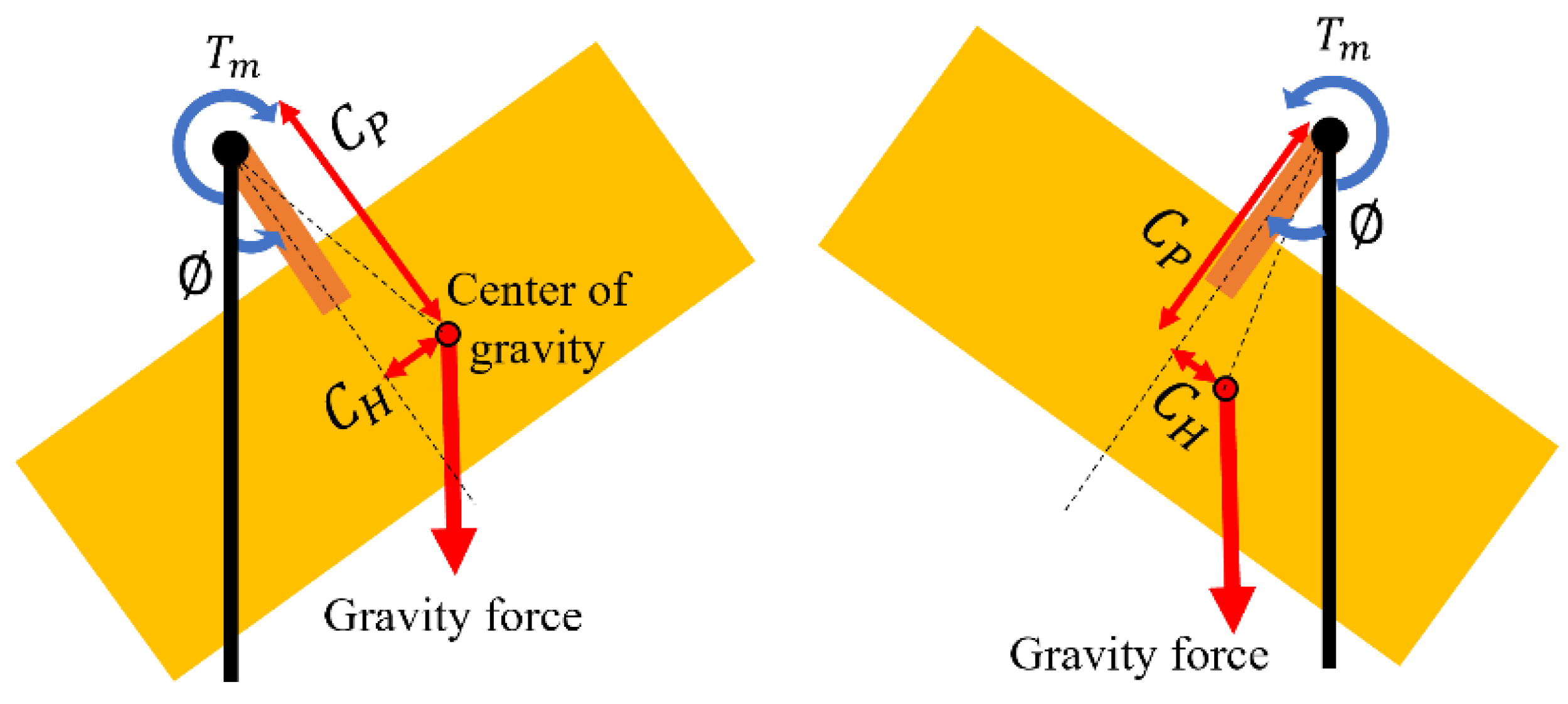
The inner frame of the 2-axes gimbal structure has much smaller properties like mass and moment of inertia than the outer frame. Also, the tilt of the loading box is mainly caused by the stair climbing of the delivery robot, and the tilt of the inner frame is insignificant. The 2-axes gimbal structure loading device is interpreted as two independent pendulum systems. This simplification is the main assumption of this paper. Each pendulum system maintains the balance by a motor located at the center of its rotation axis. The center of gravity of the loading device can change with loaded luggage. Figure 2 is the free body diagram, and Equation (1) is the dynamic equation of a pendulum structure loading device.

$$J\ddot{\varnothing }=-Mg\sqrt{C_P{}^2+C_H{}^2}\sin \left(\varnothing +{\tan }^{-1}\left(\frac{C_H}{C_P}\right)\right)+D_m\dot{\alpha }+T_m$$

(1)

• $\varnothing$: the tilt of the loading device $\left(\mathrm{degree}\right)$
• $J$: the moment of inertia of the loading device (${\mathrm{kg}\mathrm{m}}^2$)
• $M$: the mass of the loading device $\left(\mathrm{kg}\right)$
• $C_P$: the vertical position of the center of gravity from the rotate axis $\left(\mathrm{m}\right)$
• $C_H$: the horizontal position of the center of gravity from the rotate axis $\left(\mathrm{m}\right)$
• $g$: gravitational acceleration $\left(\mathrm{m}/{\mathrm{s}}^2\right)$
• $\dot{\alpha }$: angular velocity of motor shaft $\left(\mathrm{m}/s\right)$
• $D_m$: damping coefficient of the motor $\left(\mathrm{N}\mathrm{s}/\mathrm{m}\right)$
• $T_m$: $\mathrm{motor}\mathrm{torque}\left(\mathrm{N}\mathrm{m}\right)$

In Equation (1), the $\varnothing ,\dot{\alpha },$ and $T_m$ are known values that can be measured by an IMU sensor and an encoder of the motor, and the $D_m$ is determined as a fixed value by experimental data for simplifying. The $J,M,C_P$, and $C_H$ are unknown values that change depending on the loaded luggage. For system identification by a parameter estimator, the dynamic equation is expressed by dividing it into the known parameters and unknown parameters in Equations (2)–(4).

$$\ddot{\varnothing }=-\frac{Mg\sqrt{C_P{}^2+C_H{}^2}}{J}\left\{\frac{C_P\sin (\varnothing )}{\sqrt{C_P{}^2+C_H{}^2}}+\frac{C_H\cos (\varnothing )}{\sqrt{C_P{}^2+C_H{}^2}}\right\}+\frac{1}{J}\left\{D_m\dot{\alpha }+T_m\right\}$$

(2)

$$\ddot{\varnothing }=-\frac{Mg{C}_P}{J}\sin (\varnothing )-\frac{Mg{C}_H}{J}\cos (\varnothing )+\frac{1}{J}\left\{D_m\dot{\alpha }+T_m\right\}$$

(3)

$$\ddot{\varnothing }=\left[\begin{array}{ccc}\sin (\varnothing )& \cos (\varnothing )& D_m \dot{\alpha }+T_m\end{array}\right]\left[\begin{array}{c}-\frac{Mg{C}_P}{J}\\ -\frac{Mg{C}_H}{J}\\ \frac{1}{J}\end{array}\right]=N^T X=N^T \left(X_{\mathrm{empty}}+\Delta X\right)=N^T\left[\begin{array}{c}{X}_1\\ X_2\\ X_3\end{array}\right]$$

(4)

In Equation (4), the $N$ vector is the known parameters vector with measurable values, and the $X$ is the unknown parameters vector. The $X$ cannot be determined because the loaded luggage is unspecific, and it makes it difficult to design an appropriate controller. The $X$ is divided into the $X_{\mathrm{empty}}$ of the empty loading device and the $\Delta X$ which represents the difference between the empty loading device by luggage. The system identification process aims to estimate the $\Delta X$ to calculate the $X$ in real-time.

2.2. Least-Squares Method-Based System Identification Technique

The proposed system identification technique is based on the least-squares method. The parameter estimator estimates the $\Delta X$ that minimizes the error function between the ${\ddot{\varnothing }}_{\mathrm{real}}$ of the real loading device and the mathematically modeled ${\ddot{\varnothing }}_{\mathrm{model}}$ in Equation (4). The error function between the ${\ddot{\varnothing }}_{\mathrm{real}}$ and the ${\ddot{\varnothing }}_{\mathrm{model}}$ is Equation (5).

$$rr={\displaystyle \sum }_{i=1}^k{\left\{{\ddot{\varnothing }}_{\mathrm{real}}\left(i\right)-{\ddot{\varnothing }}_{\mathrm{estimated}}\left(i\right)\right\}}^2={\displaystyle \sum }_{i=1}^k\left\{{\ddot{\varnothing }}_{\mathrm{real}}\left(i\right)-N{\left(i\right)}^T\left(X_{\mathrm{empty}}+\Delta X\left(i\right)\right)\right\}{}^2$$

(5)

To minimize the $Err$, Equation (6) which is the derivative of the $Err$ should be 0. The processes of calculating the $\Delta X\left(k\right)$ when the $Err$ is 0 are Equations (7) and (8). The system identification technique estimates the $X$ in real-time by adding the $X_{\mathrm{empty}}$ and the $\Delta X\left(k\right)$ in Equation (8).

$$\frac{\partial E}{\partial \Delta X\left(k\right)}={\displaystyle \sum }_{i=1}^k\{-2N\left(i\right){\ddot{\varnothing }}_{\mathrm{real}}\left(i\right)+2N\left(i\right)N{\left(i\right)}^T{X}_{\mathrm{empty}}+2N\left(i\right)N{\left(i\right)}^T\Delta X\left(i\right)\}=0$$

(6)

$$N\left(i\right)N{\left(i\right)}^T\Delta X\left(k\right)+{\displaystyle \sum }_{i=1}^k\left\{-N\left(i\right){\ddot{\varnothing }}_{\mathrm{real}}\left(i\right)+N\left(i\right)N{\left(i\right)}^T{X}_{\mathrm{empty}}\right\}+{\displaystyle \sum }_{i=1}^{k-1}\left\{N\left(i\right)N{\left(i\right)}^T\Delta X\left(i\right)\right\}=0$$

(7)

$$\Delta X\left(k\right)={\left[N\left(k\right)N{\left(k\right)}^T\right]}^{+}[{\displaystyle \sum }_{i=1}^k\{N\left(i\right){\ddot{\varnothing }}_{\mathrm{real}}\left(i\right)-N\left(i\right)N{\left(i\right)}^T{X}_{\mathrm{empty}}\}-{\displaystyle \sum }_{i=1}^{k-1}\left\{N\left(i\right)N{\left(i\right)}^T\Delta X\left(i\right)\right\}]$$

(8)

The identification technique can estimate the dynamic equation that moves in equal motion with the real system of the loading device. The system identification technique does not need experimental results and only needs an IMU sensor and encoder of the motor. However, since there are countless solutions in calculating $\Delta X\left(k\right)$, the accuracy of the parameter estimator is sometimes poor. Although the dynamic equation that produces the equal motion with the real loading device is estimated, the large error of the parameter may cause an inappropriate controller. This is because the gain scheduler uses the unknown parameters as the inputs. As shown in ${\left[N\left(k\right)N{\left(k\right)}^T\right]}^{+}$ of Equation (8), the system identification technique is dependent on the terms of the known parameter vector $N$. Therefore, the estimation degree of each term of the $X$ varies depending on the relative size of each multiplied term of the $N$. This paper proposes an improvement in the accuracy of the parameter estimation by using a null-space solution.

2.3. System Identification Improvement Using Null-Space Solution

In the least-squares method-based system identification technique, the estimation of terms of the $X$ depends on the relative size of each term of the multiplied $N$. To adjust each term of the $N$, weights are added to the dynamic equation of the loading device. Equations (9) and (10) are the dynamic equation added by the weights.

$$\ddot{\varnothing }=X_1\{w_1+\sin (\varnothing )\}+X_2\left\{w_2+\cos (\varnothing )\right\}+X_3\left\{w_3+D_m\left(\dot{\theta }-\dot{\varnothing }\right)+{\mathrm{T}}_m\right\}-X_1{w}_1-X_2{w}_2-X_3{w}_3$$

(9)

$$\ddot{\varnothing }=\left[\begin{array}{ccc}{w}_1+\sin (\varnothing )& w_2+\cos (\varnothing )& \begin{array}{ccc}{w}_3+D_m\left(\dot{\theta }-\dot{\varnothing }\right)+{\mathrm{T}}_m& -w_1& \begin{array}{cc}-w_2& -w_3\end{array}\end{array}\end{array}\right]\left[\begin{array}{c}{X}_1\\ X_2\\ \begin{array}{c}{X}_3\\ X_1\\ \begin{array}{c}{X}_2\\ X_3\end{array}\end{array}\end{array}\right]=N^{*}{}^T X^{*}$$

(10)

The $w_1, w_2$ and $w_3$ are the weights, the $N^{*}$ is the known parameter vector, and the $X^{*}$ is the unknown parameter vector. Equation (11) is the desired solution of the $\Delta X^{*}\left(k\right)$ by adding a null-space solution to Equation (8). Equation (8) is the final equation of estimated $X$ in system identification process and it is used to optimize the controller in gain scheduling. Equations (12) and (13) is derived from Equation (8).

$$\Delta X^{*}\left(k\right)=F^{+}Z+\left(\mathrm{I}-F^{+}F\right)V=Q+R\times \mathrm{V}$$

(11)

$$F=\left[N^{*}\left(k\right)N^{*}{\left(k\right)}^T\right]$$

(12)

$$Z=[{\displaystyle \sum }_{i=1}^k\{N^{*}\left(i\right){\ddot{\varnothing }}_{\mathrm{real}}\left(i\right)-N^{*}\left(i\right)N^{*}{\left(i\right)}^T{X}_{\mathrm{empty}}^{*}\}-{\displaystyle \sum }_{i=1}^{k-1}\{N^{*}\left(i\right)N^{*}{\left(i\right)}^T\Delta X^{*}\left(i\right)\}]$$

(13)

$\left(\mathrm{I}-F^{+}F\right)V$ in Equation (11) is a null-space solution. Since the weights of Equation (10) should not affect the system of the loading device, they should be offset. The offsetting of the weights is set as a constraint to specify the null-space solution. The constraint is Equation (14). The $V$ of Equation (11) is derived as Equation (15) using this constraint. Then, the null-space solution is calculated by multiplying Equation (15) and the three rows of the $R$ in Equation (11).

$$X^{*}\left(1\right)=X^{*}\left(4\right),X^{*}\left(2\right)=X^{*}\left(5\right),X^{*}\left(3\right)=Y^{*}\left(6\right)$$

(14)

$$\begin{array}{c}\left[p\right]=Q_p,R\left[p,q\right]=R_{pq}\left(p,q=1~6\right)\\ V={\left[\begin{array}{ccc}\begin{array}{c}{R}_{11}-R_{41}\\ R_{21}-R_{51}\\ R_{31}-R_{61}\end{array}& \begin{array}{c}{R}_{12}-R_{42}\\ R_{22}-R_{52}\\ R_{32}-R_{62}\end{array}& \begin{array}{c}{R}_{13}-R_{43}\\ R_{23}-R_{53}\\ R_{33}-R_{63}\end{array}\end{array}\right]}^{+}\left[\begin{array}{c}{Q}_4-Q_1\\ Q_5-Q_2\\ Q_6-Q_3\end{array}\right]\end{array}$$

(15)

The system identification technique using a null-space solution can control the $X^{*}$ by adjusting the relative size of each term of the $N$ with the $w_1, w_2$, and $w_3$. And the accuracy of the $X_{\mathrm{estimated}}$ can be improved.

2.4. Simulation of the System Identification Techniques

The proposed system identification techniques are verified by simulation using MATLAB and Simulink (MathWorks, Natick, MA, USA). To verify the system identification, a dynamic equation assumed as a real loading device is defined in advance. The $X$ of the predefined dynamic equation is expressed as $X_{\mathrm{loaded}}$. The $X$ estimated by the least-squares method-based system identification is expressed as $X_{\mathrm{estimated}}$. $X_{\mathrm{estimated}\mathrm{NSS}}$ is the estimated $X$ by the improved system identification using a null-space solution.

Figure 3 and

Table 1. Parameters of the least-squares method-based system identification and the improved system identification with null-space solution (NSS): (a) the physical values to calculate $X_{\mathrm{empty}}$ and $X_{\mathrm{loaded}}$; (b) each term of $X_{\mathrm{empty}}$, $X_{\mathrm{loaded}}$ and $X_{\mathrm{estimated}\left(\mathrm{final}\right)}$.

		${\mathit{X}}_{\mathrm{empty}}$	${\mathit{X}}_{\mathrm{loaded}}$	${\mathit{X}}_{\mathrm{estimated} \left(\mathrm{final}\right)}$	${\mathit{X}}_{\mathrm{estimated} \mathrm{NSS}\left(\mathrm{final}\right)}$
(a)	$M$ $\left(\mathrm{kg}\right)$	0.718	5.718	-	-
	$C_P$ $\left(\mathrm{m}\right)$	0.0642	0.0683	-	-
	$C_H$ $\left(\mathrm{m}\right)$	0	0.007	-	-
	$J$ $({\mathrm{kg}\mathrm{m}}^2$)	0.0102	0.0588	-	-
(b)	$X_1\left(1/{\mathrm{s}}^2\right)$	−44.333	−65.156	−44.333	−64.552
	$X_2\left(1/{\mathrm{s}}^2\right)$	0	−6.678	−33.351	−6.740
	$X_3\left(\frac{1}{{\mathrm{kg}\mathrm{m}}^2}\right)$	98.039	17.007	84.945	17.164

show the simulation results. Figure 3a shows that the pendulum motions of the dynamic equation of the $X_{\mathrm{loaded}}$, $X_{\mathrm{estimated}}$, and $X_{\mathrm{estimated}\mathrm{NSS}}$ are equal. In Figure 3c, the $X_{\mathrm{estimated}}$ and the $X_{\mathrm{estimated}\mathrm{NSS}}$ are checked how close they are to the $X_{\mathrm{loaded}}$. Figure 3b is the torque of the motor that is related to the relative size of the terms of the $N$. Table 1 is a table that summarizes $X_{\mathrm{empty}}$, $X_{\mathrm{loaded}}$, $X_{\mathrm{estimated}\left(\mathrm{final}\right)}$, and $X_{\mathrm{estimated}\mathrm{NSS}\left(\mathrm{final}\right)}$. The $X_{\mathrm{estimated}\left(\mathrm{final}\right)}$ and $X_{\mathrm{estimated}\mathrm{NSS}\left(\mathrm{final}\right)}$ are the converged $X_{\mathrm{estimated}}$ and $X_{\mathrm{estimated}\mathrm{NSS}}$ at the stop time of the simulation. Table 1 also shows the values used in the calculation of $X_{\mathrm{empty}}$ and $X_{\mathrm{loaded}}$.

In the simulation, the movement of the stair-climbing delivery robot is a step function of 15 degrees to simulate the tilting of the frame of the roll axis which is the inner frame of the gimbal structure. A controller of the loading device is a fixed PID controller. The fixed values are as follows:

• $D_m=0.02 \mathrm{N}\mathrm{s}/\mathrm{m}$
• $g=9.81 \mathrm{m}/{\mathrm{s}}^2$
• Gains of the PID controller: $P_{\mathrm{gain}}=1.2$, $I_{\mathrm{gain}}=0.2$, $D_{\mathrm{gain}}=0.5$
• The weights: $w_1=-1.5$, $w_2=-0.5$, $w_3=-6$

In Figure 3a, the root-mean-square errors of the estimated system and the estimated (NSS) system are $4.378\times {10}^{-13}$ and $8.438\times {10}^{-13}$. It shows that the proposed system identification techniques estimate the dynamic equation that moves in equal motion with the real system.

In Figure 3c and Table 1, the $X_1$ of the $X_{\mathrm{estimated}}$ stays at the $X_{\mathrm{empty}}$. The cause is that $\sin (\varnothing )$, the first term of the known parameter vector $N$, that is multiplied by $X_1$, is almost 0 because the $\varnothing$ converges to 0. In the calculation of the $X$ by minimizing the error function of the $\ddot{\varnothing }$, the adjustment of the $X_1$ has a negligible effect, and it causes that the $\Delta X_1$ is almost 0. This problem is also shown for the $X_2$ and the $X_3$ depending on the relative size between $\cos (\varnothing )=1$, which is the second term of $N$ and motor torque in Figure 3b affecting the third term of $N$. In Table 1, the error rates of each term of the $X_{\mathrm{estimated}}$ are 31.960%, 399.427%, and 399.479%. On the other hand, the improved system identification technique using a null-space solution can adjust the $X$. The error rates of each term of the $X_{\mathrm{estimated}\mathrm{NSS}}$ are 0.928%, 0.925%, and 0.925%. The accuracy of the parameter estimation can be improved by using a null-space solution.

3. Structure of the Adaptive Controller

3.1. PID Gain Scheduler

The loading device aims to load luggage up to 5 kg and uses PID controllers for each axis to maintain the balance of the loading box. The PID controller is designed in real-time by assigning the estimated $X$ to the gain scheduler. The gain scheduler is composed of the gain scheduling function sets that use the $X_2$ and the $X_3$ as the variables. The reason why the $X_1$ is excluded is that the $X_1$ is relatively unreliable because it is multiplied by the first term of the $N$ that converged to 0. The gain-scheduling functions are defined in advance using the optimized gain sets of the PID controller. In addition, the optimized gain set is gathered while varying the $X$ to consider the changeable system of the loading device by the luggage.

The systems of each gimbal axis, that is the frame of the pitch axis and the frame of the roll axis, have different properties in terms of the empty loading box, the tilting degree of the delivery robot, demanded torque of the motor, etc. Therefore, the frames of each axis have an independent controller including not only the system identification but also the gain scheduler.

3.1.1. Gain Scheduler for the Frame of the Pitch Axis

As shown in Figure 1, the tilting degree around the pitch axis of the loading device is mainly caused by climbing the stairs of the delivery robot and it is bigger than the tilt of the roll axis. Also, the frame of the pitch axis is designed as the outer frame of the 2-axes gimbal structure loading device. As the loading device aims to handle luggage up to 5 kg, the $X$ set is composed of 6 cases of $X_3$ that have risen from the empty loading device by 1 kg each. The $X_3$ is related to the moment of inertia. Each $X_3$ is determined by the expected properties of the loading device designed by SolidWorks. Each case of the $X_3$ has 41 cases of the $X_2$, which is the divided controllable range of the motor. The $X_2$ is related to the horizontal position of the center of gravity. The optimized gains for each $X$ set are obtained by the simulation results using ‘fmincon()’ function of MATLAB that finds optimized value by minimizing the sum of errors. The $X$ set to gather the optimized gain of the frame of the pitch axis is Equation (16).

$$\begin{array}{c}0 \mathrm{kg}: X_3=10.32,\hspace{1em}{X}_2=\left[-9.5:\frac{9.5}{20}:9.5\right]\\ 1 \mathrm{kg}: X_3=9.699,\hspace{1em}{X}_2=\left[-9:\frac{9}{20}:9\right]\\ 2 \mathrm{kg}: X_3=9.017,\hspace{1em}{X}_2=\left[-8.2:\frac{8.2}{20}:8.2\right]\\ 3 \mathrm{kg}: X_3=8.190,\hspace{1em}{X}_2=\left[-7.2:\frac{7.2}{20}:7.2\right]\\ 4\mathrm{kg}: X_3=7.236,\hspace{1em}{X}_2=\left[-6.5:\frac{6.5}{20}:6.5\right]\\ 5\mathrm{kg}: X_3=6.215,\hspace{1em}{X}_2=\left[-5.5:\frac{5.5}{20}:5.5\right]\end{array}$$

(16)

Since the optimized gains show tendencies, the gain scheduler is constructed by simply interpolating the gathered gains into three-dimensional functions using the ‘fit()’ function of MATLAB. Figure 4 and Equations (18)–(20) are the gain-scheduling function for the frame of the pitch axis. The blue circles in Figure 4 are the optimized gains used to interpolate the gain-scheduling function. In interpolating the gains, the normalization function is included to consider cases of the $X_2$ close to zero, and it is shown in Equation (17).

$$x=\frac{X_2}{4.61}, y=\frac{X_3-8.446}{1.412}$$

(17)

$$\begin{array}{c}{P}_{\mathrm{gain}}=2.376-0.0426 x-0.257 y+2.315 x^2+0.02246 x y+0.05377 x^3-0.6863 x^2 y-0.6768 x^4\\ +0.01042 x^3 y-0.01188 x^5+0.3795 x^4 y\end{array}$$

(18)

$$\begin{array}{c}{I}_{\mathrm{gain}}=0.06586-0.001902 x-0.01197 y+0.03357 x^2+0.0006987 x y+0.0003353 x^3-0.01913 x^2 y\\ -0.01175 x^4-0.0006846 x^3 y+0.0002325 x^5+0.007949 x^4 y\end{array}$$

(19)

$$\begin{array}{c}{D}_{\mathrm{gain}}=0.8144-0.008396 x-0.1647 y-0.002875 x^2+0.002468 x y+0.007287 x^3-0.003321 x^2 y\\ +0.02428 x^4-0.001404 x^3 y-0.0006309 x^5-0.003238 x^4 y\end{array}$$

(20)

3.1.2. Gain Scheduler for the Frame of the Roll Axis

The tilting degree around the roll axis of the loading device is mainly caused by the slope of one jaw of the stair, and it is smaller than the tilt of the pitch axis. The frame of the roll axis is the inner frame of the gimbal structure. The $X$ set to gather the optimized gain of the frame of the roll axis is Equation (21).

$$\begin{array}{c}0 \mathrm{kg}: X_3=98.039,\hspace{1em}{X}_2=\left[-29.5:\frac{29.5}{20}:29.5\right]\\ 1 \mathrm{kg}: X_3=66.445,\hspace{1em}{X}_2=\left[-29.5: \frac{29.5}{20}:29.5\right]\\ 2 \mathrm{kg}: X_3=50.251,\hspace{1em}{X}_2=\left[-22:\frac{22}{20}:22\right]\\ 3 \mathrm{kg}: X_3=33.784,\hspace{1em}{X}_2=\left[-15:\frac{15}{20}:15\right]\\ 4\mathrm{kg}: X_3=25.445,\hspace{1em}{X}_2=\left[-11:\frac{11}{20}:11\right]\\ 5\mathrm{kg}: X_3=20.367,\hspace{1em}{X}_2=\left[-9:\frac{9}{20}:9\right]\end{array}$$

(21)

In the results of the simulation to obtain the optimized gain set, the $P_{\mathrm{gain}}$ converges in the initial setting value in several simulations. In the case of the frame of the roll axis, the adjustment of $P_{\mathrm{gain}}$ is an insignificant effect because the allowed error is limited by the outer frame of the gimbal being small. The gain scheduler of the frame of the roll axis adapts the I and D gain by the gain-scheduling functions and uses a fixed $P_{\mathrm{gain}}$. Figure 5 and Equations (23) and (24) are the PID gain-scheduling function for the frame of the roll axis. The normalization of interpolating the gains is shown in Equation (22).

$$x=\frac{X_2}{12.46}, y=\frac{X_3-49.06}{26.88}$$

(22)

$$\begin{array}{cc}\hfill I_{\mathrm{gain}}=0.02152& -0.0001089 x-0.01084 y+0.003878 x^2+0.0001591 x y+0.004848 y^2-0.000337 x^2 y\hfill \\ & -0.001033 y^3-0.0005136 x^4-0.0002505 x^3 y-0.001298 x^2 y^2+0.0001455 x y^3\hfill \\ & +0.002524 y^4+0.000275 x^4 y+0.0001112 x^3 y^2+0.0003705 x^2 y^3-0.0001177 x y^4\hfill \\ & -0.001327 y^5\hfill \end{array}$$

(23)

$$\begin{array}{cc}\hfill D_{\mathrm{gain}}=0.1975& +0.0001443 x-0.09851 y+-0.002835 x^2-0.002265 x y+0.07358 y^2+0.0004731 x^3\hfill \\ & +0.01318 x^2 y-0.002979 x y^2-0.02471 y^3-0.0005513 x^4-0.0001227 x^3 y\hfill \\ & -0.005469 x^2 y^2+0.002157 x y^3\hfill \end{array}$$

(24)

3.2. Structure of the Adaptive Controller

According to Section 2.3, the improved system identification technique using a null-space solution should adjust the weights $w_1, w_2$ and $w_3$. The $w_1$ and $w_3$ are determined by each function that uses the motor torque as the variable. On the contrary, $w_2$ is almost fixed as $\varnothing$ is almost 0, so the relative sizes of each term of the $N$ can be adjusted. Therefore, the $X_{\mathrm{estimated}}$ can be derived to produce an appropriate controller for each demanded motor torque. Equations (25) and (26) are functions of each weight of the pitch axis and the roll axis.

$$\mathrm{pitch}\mathrm{axis}:w_1=-\frac{1.2 T_m}{0.9},\hspace{1em}{w}_2=-\frac{\cos (\varnothing )}{2},\hspace{1em}{w}_3=-\frac{0.3 T_m}{0.9}$$

(25)

$$\mathrm{oll}\mathrm{axiz}:w_1=-\frac{1.2 T_m}{0.4},\hspace{1em}{w}_2=-\frac{cos(\varnothing )}{2},\hspace{1em}{w}_3=-\frac{5.3 T_m}{0.4}$$

(26)

The controller also includes a smoothing filter and anti-wind-up technique. The smoothing filter is intended to prevent instability due to overly sensitive parameter estimations of system identification. The anti-wind-up technique is intended to remove the accumulated error due to external force or other reasons. Figure 6 is the block diagram of the proposed adaptive control strategy.

In summary of the proposed adaptive control strategy, the parameter estimator for system identification estimates the unknown parameter of the dynamic equation with only an IMU and an encoder of the motor. Then, the gain scheduler determines the gains of the controller using the estimated unknown parameter filtered stably by the smoothing filter. After the PID gains are determined, and the motor can control the balance of the loading device with the appropriate controller. Additionally, the anti-wind-up technique helps to remove unexpected and accumulated errors.

4. Experiments

4.1. Experimental Apparatus

Figure 7 is the designed loading device. The designed loading device is divided into a balancing module and a positioning module. The balancing module has a 2-axes gimbal structure with flat motors. The positioning module moves the position of the loading box by a ball screw set for the more stable operation of the delivery robot. An IMU sensor is included to measure the tilt of the loading box.

4.2. Experimental Progress

A motion platform is used in the experiments instead of a delivery robot. This paper shows the results of three experiments. The motions of the motion platform of each experiment are equal, titling and returning 20 degrees around the pitch axis and 15 degrees around the roll axis at the same time. Each experiment handles luggage with different mass and loaded positions. One experiment is with the empty loading device, one is with 3 kg luggage in an offset position, and the other is with 5 kg luggage. Figure 8 is the picture of the experiments.

4.3. Results of Experiments

Figure 9 and Figure 10 show the experimental results. Figure 9 is for the frame of the pitch axis and Figure 10 is for the frame of the roll axis. Figure 9a and Figure 10a show the tilt of the loading box and the motion platform in one graph. Figure 9b and Figure 10b show the ${\ddot{\varnothing }}_{\mathrm{real}}$ of the real loading device and the ${\ddot{\varnothing }}_{\mathrm{estimated}}$ of the system identification.

Figure 9a.1,b.1 and Figure 10a.1,b.1 are the results of the experiment with the empty loading device. Figure 9a.2,b.2 and Figure 10a.2,b.2 are the graphs of experiment with 3 kg luggage in an offset position, the back of the loading box. Figure 9a.3,b.3 and Figure 10a.3,b.3 are from the experiment with 5 kg luggage. Figure 9c and Figure 10c compare the scheduled PID gains of each experiment in one graph. Figure 9c.1 shows P gains, Figure 9c.2 shows I gains, and Figure 9c.3 shows D gains. Figure 10c.1 shows I gains and Figure 10c.2 shows D gains. The P gain of the frame of the roll axis is fixed at 1.2 derived as the optimized gain by the experimental results in advance.

All of the root-mean-square errors of the angular acceleration of the real loading device and estimated dynamic equation in Figure 9b and Figure 10b are 0. The parameter estimator by the least-squares method-based system identification technique works properly and estimates the dynamic equation of equal motion with the real loading device.

In Figure 9c and Figure 10c, the gains of the experiments are scheduled by the estimated $X_2$ and $X_3$, and adapt to the system of the loading device in real-time. The luggage of each experiment has fixed properties like mass, moment of inertia, and position of center of gravity during the experiments. In Figure 9c and Figure 10c, all PID gains change during each experiment. It means the estimated parameter in system identification changes although the system has fixed properties. As end of Section 2.2 explained, the reason is that the estimating parameter of Equation (11) in system identification has countless solution. The main goal of the proposed control strategy is not to estimate the system correctly, but to optimize the controller for balancing loading device. Therefore, in the system identification process, the weights for a null-space solution are determined by the motor torque to derive appropriate PID gains for the required torque. As shown in Figure 9a,c and Figure 10a,c, the change in the gains occurs when the motion platform changes the tilt. In Figure 11 which shows the motor torque of each experiment, the tilt motion of the motion platform causes additional torque to maintain the balance of the loading box. Therefore, to optimize the controller in real-time in response to sudden movement or other disturbance, the PID gains also change during each experiment using luggage of fixed properties.

As shown in Figure 9c, the PID gains for the experiment with the 3 kg luggage is larger than the experiment with the 5 kg luggage. The reason can be explained in Figure 11a, which shows the motor torque of each experiment for the frame of the pitch axis. As shown in Figure 11a, the absolute value of the motor torque of the experiment with 3 kg is larger than the 5 kg experiment. This is because the 3 kg luggage is positioned in the offset location, and it causes the additional torque to maintain the balance of the loading box. Therefore, the PID gains for 3 kg luggage positioned at the back of the loading box should be larger. Likewise, gains of the experiment with the empty loading device are the lowest. It is because the demanded torque of the empty loading box is much lower than the cases of loading the 3 kg and 5 kg luggage. In conclusion, the proposed adaptive control strategy can adapt the controller to the system of the loading device.

Table 2. Largest overshoot and longest settling time of each experiment.

		The Empty Loading Device	Load 3 kg in Offset Position	Load 5 kg
Pitch	$\mathrm{Overshoot}\left(\mathrm{degree}\right)$	1.7	1.21	1.77
	$\mathrm{Settling}\mathrm{time}\left(\mathrm{s}\right)$	0.64	2.11	2.19
Roll	$\mathrm{Overshoot}\left(\mathrm{degree}\right)$	1.18	1.45	2
	$\mathrm{Settling}\mathrm{time}\left(\mathrm{s}\right)$	1.67	2.45	2.1

shows the largest overshoot and the longest settling time of each experiment in Figure 9a and Figure 10a. The error rate of settling time is 5%. The starting point of the measurement of settling time is from when the motion platform starts the tilting. In Figure 9 and Figure 10, and Table 2, the frame of the roll axis seems to be worse controlled than the frame of the pitch axis with vibration and longer convergence times to 0. The cause is considered that the gimbal structure is interpreted as two independent pendulum systems in the system identification process. Also, the frame of the roll axis is the inner frame of the gimbal structure, and it is relatively more affected by the motion of the outer frame. It may cause more instability. However, considering that there are two rapid angular acceleration changes in one tilting motion of the motion platform, the balance maintenance control of the frame of the roll axis works well by the adaptive control strategy.

5. Conclusions

This paper proposes an adaptive control strategy including system identification and gain scheduling. The system identification is conducted by parameter estimation based on least-squares method, and it estimates the unknown parameters of the dynamic equation of the loading device. In the simulation, the root-mean-square error between the motions of a predefined system and the estimated system is almost 0. This means that the least-squares method-based system identification technique estimates the dynamic equation that moves in equal motion with the real loading device. The accuracy of the parameter estimation of the system identification technique is improved using a null-space solution. Compared to the parameter estimation of the normal system identification technique showing error rates of 31.960%, 399.427%, 399.479%, the improved system identification technique shows error rates of 0.928%, 0.925%, 0.925%. In the proposed adaptive control strategy, the weights for the null-space solution are determined by the motor torque. Therefore, the parameter estimator can respond appropriately to the demanded torque in the gain scheduling process.

The PID gain scheduling for the frames of the pitch axis and the roll axis uses independent gain schedulers for each axis. Each gain scheduler consists of surface functions using the estimated unknown parameters in the system identification process as the variables. The surface functions are constructed in advance by interpolating the optimized gains. The gain scheduler can adapt the controller by assigning the unknown parameters to the scheduling surface functions in real-time. In the case of the structure of the controller, it includes not only a system identification and a gain scheduler but also a smoothing filter and anti-wind-up technique.

The experiments using a motion platform are conducted. In the results of the experiments, the root-mean-square error between the angular accelerations of the real loading device and the estimated system is 0. The gain scheduler properly adapts the controller depending on the motor torque in real-time. In the case of the balancing control of the loading box, every overshoot and settling time of 5% error rate of all experiments are 2 degrees and 2.45 s or less. The 2-axes gimbal loading device is well balanced by the proposed adaptive control strategy despite the tilting of the motion platform and system change caused by the luggage.

The next step of this study is to apply the loading device to a stair-climbing delivery robot. The loading device should be lighter, and carefully adjust the position of the center of gravity for the stable operation of the delivery robot.

References

1. Gautam, P. System identification of nonlinear Inverted Pendulum using artificial neural network. In Proceedings of the 2016 International Conference on Recent Advances and Innovations in Engineering (ICRAIE), Jaipur, India, 23–25 December 2016; pp. 1–5. [Google Scholar] [CrossRef]
2. Arévalo-Castiblanco, M.F.; Rodríguez-Garavito, C.H.; Patiño-Forero, A.A. Identification of a non-linear model type inverted rotary pendulum. In Proceedings of the 2017 IEEE 3rd Colombian Conference on Automatic Control (CCAC), Cartagena, Colombia, 18–20 October 2017; pp. 1–6. [Google Scholar] [CrossRef]
3. Qi, Q.; Huang, W.; Zhao, Y.; He, Q.; Huang, Q.; Lin, X. System identification of the double inverted pendulum based on genetic algorithm. In Proceedings of the 2008 2nd International Symposium on Systems and Control in Aerospace and Astronautics, Shenzhen, China, 10–12 December 2008; pp. 1–5. [Google Scholar] [CrossRef]
4. Harati, M.; Ghavifekr, A.A.; Ghiasi, A.R. Model Identification of Single Rotary Inverted Pendulum Using Modified Practical Swarm Optimization Algorithm. In Proceedings of the 2020 28th Iranian Conference on Electrical Engineering (ICEE), Tabriz, Iran, 4–6 August 2020; pp. 1–5. [Google Scholar] [CrossRef]
5. Hu, C.; Wan, F. Parameter identification of a model with Coulomb friction for a real Inverted Pendulum System. In Proceedings of the 2009 Chinese Control and Decision Conference, Guilin, China, 17–19 June 2009; pp. 2869–2874. [Google Scholar] [CrossRef]
6. Barket, A.; Hamayun, M.T.; Ijaz, S.; Akhtar, S.; Ansari, E.A.; Ghous, I. Model identification and real-time implementation of a linear parameter-varying control scheme on lab-based inverted pendulum system. J. Syst. Control Eng. 2021, 235, 33–38. [Google Scholar] [CrossRef]
7. Sim, Y.; Jin, S. Least squares method-based system identification for a 2-axes gimbal structure loading device. J. Korea Robot. Soc. 2022, 17, 288–295. [Google Scholar] [CrossRef]
8. Flacco, F.; De Luca, A.; Khatib, O. Motion control of redundant robots under joint constraints: Saturation in the Null Space. In Proceedings of the 2012 IEEE International Conference on Robotics and Automation, Saint Paul, MN, USA, 14–18 May 2012; pp. 285–292. [Google Scholar] [CrossRef]
9. Sadeghian, H.; Villani, L.; Keshmiri, M.; Siciliano, B. Task-Space Control of Robot Manipulators With Null-Space Compliance. IEEE Trans. Robot. 2021, 30, 493–506. [Google Scholar] [CrossRef]
10. Platt, R.; Fagg, A.H.; Grupen, R.A. Null-Space Grasp Control: Theory and Experiments. IEEE Int. Trans. Robot. 2010, 26, 282–295. [Google Scholar] [CrossRef]
11. Antonelli, G.; Arrichiello, F.; Chiaverini, S. The null-space-based behavioral control for autonomous robotic systems. Intell. Serv. Robot. 2008, 1, 27–39. [Google Scholar] [CrossRef]
12. Fauzi, B.A.; Khisbullah, H.; Hishamuddin, J. Gain scheduling PID control with pitch moment rejection for reducing vehicle dive and squat. Int. J. Veh. Saf. 2009, 4, 45–83. [Google Scholar] [CrossRef]
13. Poksawat, P.; Wang, L.; Mohamed, A. Gain Scheduled Attitude Control of Fixed-Wing UAV With Automatic Controller Tuning. IEEE Trans. Control Syst. Technol. 2018, 26, 1192–1203. [Google Scholar] [CrossRef]
14. Luna, A.L.; Vega, I.C.; Carranza, J.M. Gain-Scheduling and PID Control for an Autonomous Aerial Vehicle with a Robotic Arm. In Proceedings of the 2018 IEEE 2nd Colombian Conference on Robotics and Automation (CCRA), Barranquilla, Colombia, 1–3 November 2018; pp. 1–6. [Google Scholar] [CrossRef]
15. Melo, A.G.; Andrade, F.A.A.; Guedes, I.P.; Carvalho, G.F.; Zachi, A.R.L.; Pinto, M.F. Fuzzy Gain-Scheduling PID for UAV Position and Altitude Controllers. Sensors 2022, 22, 2173. [Google Scholar] [CrossRef] [PubMed]
16. Ghafari, A.S.; Alasty, A. Design and real-time experimental implementation of gain scheduling PID fuzzy controller for hybrid stepper motor in micro-step operation. In Proceedings of the IEEE International Conference on Mechatronics, Istanbul, Turkey, 5 June 2004; pp. 421–426. [Google Scholar] [CrossRef]
17. Kumar, A.; Kumar, A.; Chanana, S. Genetic fuzzy PID controller based on adaptive gain scheduling for load frequency control. In Proceedings of the 2010 Joint International Conference on Power Electronics, Drives and Energy Systems & 2010 Power India, New Delhi, India, 20–23 December 2010; pp. 1–8. [Google Scholar] [CrossRef]
18. Zhang, J. A nonlinear gain scheduling control strategy based on Neuro-Fuzzy networks. Ind. Eng. Chem. Res. 2001, 40, 3164–3170. [Google Scholar] [CrossRef]
19. Bouguerra, A.; Saigaa, D.; Kara, K.; Zeghlache, S. Fault-tolerant Lyapunov-gain-scheduled PID control of a quadrotor UAV. Int. J. Intell. Eng. Syst. 2015, 8, 1–6. [Google Scholar] [CrossRef]
20. Anh, H.P.H. Online tuning gain scheduling MIMO neural PID control of the 2-axes pneumatic artificial muscle (PAM) robot arm. Expert Syst. Appl. 2010, 37, 6547–6560. [Google Scholar] [CrossRef]
Figure 1. Concept figure of a delivery robot and a 2-axes gimbal structure loading device.
Applsci 12 09214 g001
Figure 2. Free body diagram of a pendulum structure loading device.
Applsci 12 09214 g002
Figure 3. Simulation results of the least-squares method-based system identification and the improved system identification with null-space solution (NSS): (a) the tilt of the loading device and the delivery robot; (b) the motor torque for balancing control of the loading device; (c) the X estimated   NSS , X estimated and the X loaded : (c.1) the X 1 , the first term of X ; (c.2) the X 2 , the second term of X ; (c.3) the X 3 , the third term of X .
Applsci 12 09214 g003
Figure 4. Gain-scheduling three-dimensional functions for the frame of the pitch axis of the loading device: (a) P gain scheduler; (b) I gain scheduler; (c) D gain scheduler.
Applsci 12 09214 g004
Figure 5. Gain-scheduling three-dimensional functions for the frame of the roll axis of the loading device: (a) I gain scheduler; (b) D gain scheduler.
Applsci 12 09214 g005
Figure 6. Block diagram of the adaptive control strategy.
Applsci 12 09214 g006
Figure 7. Design of the loading device for stair-climbing delivery robot.
Applsci 12 09214 g007
Figure 8. Experiment of the loading device: (a) the experiment with the empty loading device; (b) the experiment with luggage (5 kg).
Applsci 12 09214 g008
Figure 9. Experimental result for the frame of the pitch axis: (a) the tilt of the loading device and the motion platform: (a.1) the empty loading device experiment; (a.2) load 3 kg luggage in the offset position; (a.3) load 5 kg luggage; (b) the angular accelerations of the real loading device and the estimated system by the system identification: (b.1) the empty loading device experiment; (b.2) load 3 kg luggage in the offset position; (b.3) load 5 kg luggage; (c) the scheduled gains of controller of each experiment: (c.1) P gain; (c.2) I gain; (c.3) D gain.
Applsci 12 09214 g009
Figure 10. Experimental result for the frame of the roll axis: (a) the tilt of the loading device and the motion platform; (a.1) the empty loading device experiment; (a.2) load 3 kg luggage in the offset position; (a.3) load 5 kg luggage; (b) the angular accelerations of the real loading device and the estimated system by the system identification: (b.1) the empty loading device experiment; (b.2) load 3 kg luggage in the offset position; (b.3) load 5 kg luggage; (c) the scheduled gains of controller of each experiment: (c.1) I gain; (c.2) D gain.
Applsci 12 09214 g010
Figure 11. Motor torque of the frames of each axis; (a) the pitch axis; (b) the roll axis.
Applsci 12 09214 g011