Abstract
Forecasting the aggregate charging load of a fleet of electric vehicles (EVs) plays an important role in the energy management of the future power system. Therefore, accurate charging load forecasting is necessary for reliable and efficient power system operation. A hybrid method that is a combination of the similar day (SD) selection, complete ensemble empirical mode decomposition with adaptive noise (CEEMDAN), and deep neural networks is proposed and explored in this paper. For the SD selection, an extreme gradient boosting (XGB)-based weighted k-means method is chosen and applied to evaluate the similarity between the prediction and historical days. The CEEMDAN algorithm, which is an advanced method of empirical mode decomposition (EMD), is used to decompose original data, to acquire intrinsic mode functions (IMFs) and residuals, and to improve the noise reduction effect. Three popular deep neural networks that have been utilized for load predictions are gated recurrent units (GRUs), long short-term memory (LSTM), and bidirectional long short-term memory (BiLSTM). The developed models were assessed on a real-life charging load dataset that was collected from 1000 EVs in nine provinces in Canada from 2017 to 2019. The obtained numerical results of six predictive combination models show that the proposed hybrid SD-CEEMDAN-BiLSTM model outperformed the single and other hybrid models with the smallest forecasting mean absolute percentage error (MAPE) of 2.63% Canada-wide.
Keywords:
EV; charging load; SD selection; CEEMDAN; GRU; LSTM; BiLSTM; short-range EV; mid-range EV; long-range EV 1. Introduction
1.1. Problem Statement
The global EV market is growing exponentially. The World Economic Forum says worldwide sales of EVs reached 6.6 million in 2021, almost doubling from the previous year [1]. The International Energy Agency estimated that the global EV fleet could reach 250 million by 2030 [2]. With the significant growth of the EV industry, it is bound to bring new challenges to the power systems due to the large battery capacity and uncertain charging behaviors of EV users [3]. This would result in significant peak–valley differences in load in featured time slots, particularly in a super-short-term time scale. Therefore, utilities and other power producers need to be prepared to meet the increased loads as transportation electrification grows, and to be able to forecast required electricity with a minimum error, to maintain stable and effective power system operation.
1.2. Proposed Solutions
Over the past few decades, scientists have proposed various solutions to improve the accuracy of short-term load forecasting (STLF) methods including traditional methods, the SD selection, the EMD methods, artificial intelligence (AI), and hybrid forecasting models [4,5,6,7,8,9,10,11,12,13]. With energy grid diversification, an increasing number of factors impact the load demand such as weather, holidays, and electricity prices [3]. Traditional load forecasting methods are unable to provide prediction models with sufficient accuracy [14]. These models are based on mathematical methods that often perform poorly when predicting non-linear problems [15].
The SD selection is based on historical days that have comparable features to capture the features of load. To predict short-term load, a weekday index and weather events similar to the forecasted day were used [16]. The SD selection was applied to assess the attribute weights using the XGB algorithm and to compute the distance between the chosen day and the day that depends on different measurement attributes in different weights [12]. The authors also used the k-means algorithm to merge SDs into one cluster and applied it as input data for the succeeding load prediction based on the XGB distance. However, scientists found that the SD method cannot sufficiently capture the complex electric load features alone and it should be combined with other methods [12,16,17,18].
AI and machine learning (ML) modeling techniques are broadly used by many electric utility companies to handle accurate load forecasting problems [19]. Although comprehensive research has been accomplished, accurate STLF remains a challenge due to its non-stationary electric load data and long-term dependencies estimating horizon [12]. The LSTM model, which is a special type of recurrent neural network (RNN), was used to predict the aggregated demand-side electric load over the short- and medium-term horizons [20]. The BiLSTM has been applied in several areas of study to provide accurate aggregated electric load prediction results [21,22,23]. The GRU model was used to forecast the short-term load of EV charging stations and the state of charge of batteries [3,24]. A comparative study of ML approaches using LSTM, BiLSTM, and GRU was evaluated for day-ahead charging of the EV fleet in Canada [25]. The results showed that the BiLSTM algorithm has the lowest error among the used models and was best suited for load prediction of the EV fleet. However, in view of the complexity and non-stationarity of the aggregate load of the EV fleet, it is difficult to obtain accurate results using neural networks.
The EMD method has been used by many scholars in a wide range of applications including electric load, wind speed, solar radiation, and crude oil price to improve prediction accuracy [5,6,7,12,26,27]. The EMD method can sufficiently extract the features of the original data from non-stationary and unstable time series into a series of frequency components [28]. There are many types of EMD methods that can be applied to the time series including ensemble EMD (EEMD), complete EEMD (CEEMD), and CEEMD with adaptive noise (CEEMDAN). Compared with EMD and EEMD, the CEEMDAN method can perform a better spectral separation of the IMFs at a lower computational cost [29]. More recently, CEEMDAN was used to reconstruct the original input/output variables for electricity demand forecasting [30]. They found that the accuracy of the load model with the CEEMDAN method is greater than that without it.
Based on the above-mentioned solutions, a hybrid approach consisting of the SD selection, the CEEMDAN, and deep neural networks is proposed to forecast the aggregated load of an EV fleet. The SD method is used to capture the features of load using the XGB algorithm and cluster them using the k-means method. The CEEMDAN technique is introduced to decompose historical data into a set of IMFs and a residue. Three ML methods comprising LSTM, BiLSTM, and GRU were applied to compare and select the best-suited method for predicting the charging load of the EV fleet.
The contribution of the presented paper is the application of the CEEMDAN, the SD methods, and deep neural networks applied to the problem of STLF in EV fleet research with:
- a unique heterogeneous fleet of 1000 EVs, grouped into long-range, mid-range, and short-range EVs, in terms of their battery capacity;
- the three-day-ahead predictions with high accuracy achieved on real data provided by FleetCarma Inc. (Waterloo, ON, Canada);
- an evaluation with various methods comprising the SD selection, the CEEMDAN method, and different RNN architectures.
2. Materials and Methods
This section describes the SD approach, the signal-processing algorithm called CEEMDAN, and the three structures of RNN comprising LSTM, BiLSTM, and GRU investigated in this study.
2.1. SD Approach Using XGB and k-Means
This section estimates the weights of the features, i.e., vehicle groups, charging levels, charging locations, temperature, electricity rates, seasonal category, weather events, day type, etc. [25], using the XGB algorithm. Then, the weighted features are integrated using the k-means clustering.
XGB is a decision tree-based ensemble ML algorithm that applies a gradient boosting framework. XGB is a supervised algorithm that assembles all base learners into strong learners. The prediction result by XGB is equal to the total of all base learners.
The XGB process is as follows:
where represents the nth decision tree, N is the number of decision trees, F is the space that covers a set of decision trees. The objective function of XGB includes the loss function and the regularization term, which are defined as:
where denotes the loss function, are the prediction and the target values, states the regularization term, n is the number of targets , specifies the leaf node number in a decision tree, is the score of leaf nodes, γ and β act as the penalty factors. Then, k-means clustering, which is an unsupervised learning algorithm, is used to partition n observations into different clusters, so that similar data points are grouped together and underlying patterns can be discovered.
2.2. Complete Ensemble Empirical Mode Decomposition with Adaptive Noise (CEEMDAN)
CEEMDAN is an algorithm based on EMD [31], that can effectively solve the EMD mode mixing and the EEMD residual noise problems. The decomposition process is as follows:
- i.
- Add white noise with a normal distribution to the original signal The signal for the ith decomposition, where i denotes the number of decompositions, is represented as
- ii.
- The EMD decomposes the trial signal Si(t) to obtain correspondingly, so
- iii.
- Add white noise to the residual , execute the trial i times (i = 1, 2, ⋯, I), and each trial adopts EMD to decomposeto find its first-order component .Residual
- iv.
- Then, the signal is further decomposed by EMD to calculate the second IMF mode and the relating residue by repeating the above decomposition process. When the residual cannot be decomposed by EMD, the program ends. The original signal can be represented as:
2.3. Long Short-Term Memory (LSTM) and Bidirectional LSTMs
LSTM is a specific RNN architecture used to prevent gradient vanishing and exploding problems. LSTMs can acquire long-term dependencies by a gate mechanism that can control the flow of information. These gates can realize which data in the sequence are important to preserve or forget. There are three different gates in the LSTM cell; input, forget, and output (Figure 1).
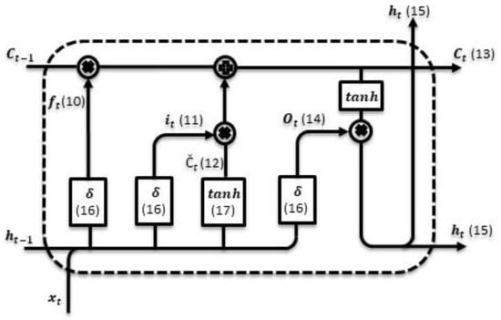
Figure 1.
The architecture of LSTM cell. Numbered values correspond to the equation numbers below.
The following equations are the LSTM cell states and parameters’ updating scheme [12,20,32]:
where and represent the activation of input, forget, and output gate at time step t, respectively, is the output at time step , is the input at the present moment, and is the memory cell from the previous state. The forget gate () can input the information in and , and outputs a vector, with values ranging from 0 to 1 for the cell state , 1 means completely reserved and 0 means completely discarded. The input gate decides what new information is going to be stored in the cell state, and the first part is the sigmoid layer called the “input gate layer” that decides which values will be updated. The second part is that the layer creates a vector of a new candidate value, which is added to the state. The current block memory is created by the accumulation of the items from the previous block and input gate. Finally, the output gate () determines the cell state value, where W and b are weight and bias. The following equations are sigmoid and hyperbolic tangent functions
The idea of BiLSTM is to combine input information in the past and future time step in LSTM models. In BiLSTM, information can be preserved from both the past and future at any point in time [33].
2.4. Gated Recurrent Unit (GRU)
GRU is a newer generation of RNN architecture and is similar to LSTM. GRU does not have the cell state, instead it uses a hidden state to transfer information. Therefore, GRU has only two gates: reset and update gate (Figure 2).
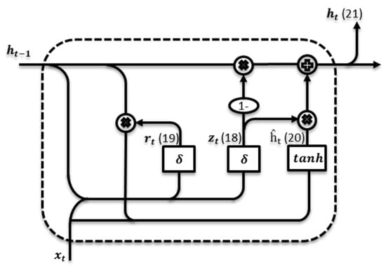
Figure 2.
The architecture of the GRU cell. Numbered values correspond to the equation numbers below.
The key equations for GRU are shown below [24]:
where and are input, output, activation function, update gate, and reset gate. W, U, and b are parameter matrices and vectors.
and are sigmoid and hyperbolic tangent functions. GRUs have fewer parameters and thus may train faster than LSTM.
2.5. The Proposed SD-CEEMDAN-BiLSTM Prediction Model
In the BiLSTM model, the rectified linear unit (ReLU) function is used as an activation function of the stack of a fully connected layer and the mean square error (MSE) is used as a loss function.
where is the sum of estimated number of days, is the estimated value, and is the actual value.
The proposed model generally comprises the following steps, which are shown in Figure 3.
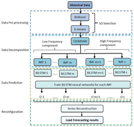
Figure 3.
Hybrid forecast model based on SD-CEEMDAN-BiLSTM.
- I.
- The feature weight is calculated by the XGB method and is merged with the k-means algorithm to establish the SD cluster.
- II.
- The CEEMDAN method is utilized to decompose the charging load into several IMF sequences (i = 1, 2, ⋯, M) and one residue .
- III.
- Each IMF and the residue item are normalized and used as the input to the BiLSTM model for training and obtaining the predicted values, respectively. The results of the test set predictions are (i = 1, 2, ⋯, M) and
- IV.
- Then, the final forecast results are adjusted using the below formula.where L is the test series length, and is the final predictive series of the test set.
The architecture of the BiLSTM was derived by testing different configurations of units in each layer and calculating the MAPE on training and testing datasets. Table 1 shows the MAPE for a different number of layers and units for data with one-day-ahead prediction. Increasing the capacity of the neural network can be seen by increasing the number of layers and units, which improves error on the training and testing dataset. However, the proposed model executes well on the training data by a 2-layer network with 100 units in layer 2 and 30 units in layer 1.

Table 1.
MAPE (%) of the proposed model architecture.
3. Data Pre-Processing and Feature Analysis
3.1. Data Description and Input Variable
A large dataset with over 727,000 charging load events was collected in nine provinces in Canada (Figure 4) by FleetCarma Inc., in partnership with 10 electric utility companies and the University of Waterloo, over a three-year period using FleetCarma data loggers via the OBD II port of 1000 EVs. The collected data include charging loads of thirty-five vehicle models for three charging locations and three charging levels. The data include charging load start and end times, energy consumption, energy loss, and the state of charge of the battery at start time and end time.
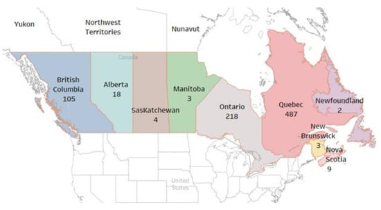
Figure 4.
Number and distribution of EVs used in this project.
For the charging load prediction, two individual models were developed to process battery size and weather events into feature input parameters, and the full results have been published recently [25].
3.2. XGB Feature Importance
Several features described in Section 2.1 are used as inputs for the XGB algorithm to compute the feature importance with a charging load for a fleet of EVs (Figure 5). The increase in the feature importance of the individual predictors in the tree is then visualized. A higher value of the metric “Feature gain score”, compared to another feature, implies it is more important for generating a prediction. It can be seen from Figure 5 that the charge load is sensitive to temperature variables. In addition, the SD charging load, which has the highest feature gain score, is an important feature for load prediction. This assumption is consistent with the data analysis results.
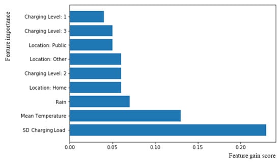
Figure 5.
XGB feature importance.
3.3. Data Decomposition
The CEEMDAN method is utilized to decompose the aggregated charging load at low- and high-frequency waves, which correspond to daily and seasonal, respectively. All graphs in Figure 6 are on the same scale, thus enabling the evaluation of the contribution of each extracted IMF on the daily, weekly, monthly, and seasonal scales (Figure 6b–e). It can be seen that increasing the range of data for decomposition from daily to seasonally would decrease the amplitude of the fluctuation. Therefore, it presents improvements in the extracted IMFs and provides a valuable abstract for data visualization. For load forecasting, the generated IMFs were divided into training and testing sets, with the ratio selected as 76/24 (16 months of training data, and 5 months of testing data).
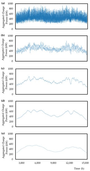
Figure 6.
The original data sequence of the aggregated daily charging load (a) and the result of CEEMDAN; daily (b) weekly (c), monthly (d), seasonally (e).
For time interval processing, Anaconda, which is a distribution of the Python programming language, was used to integrate all the charging load event data based on the time stamps and split them into 24 h time stamps every single day.
3.4. Evaluation Indicators
To evaluate the performance of the models and the prediction errors, three commonly used metrics, including root mean squared error (RMSE), mean absolute error (MAE), and mean absolute percent error (MAPE), were employed. The error indicators are defined as below:
where is the actual value, is the prediction value, and N is the total amount of data.
4. Results
Six predictive combination models including the SD selection, the CEEMDAN method, and three different RNN architectures (GRU, LSTM, BiLSTM) were selected for comparative analysis and for verifying the predictive performance of the proposed model. The six predictive combination models in this research are implemented using Python Anaconda.
Figure 7 and Figure 8 illustrate the results of the aggregated charge power, in kilowatts (kW), during the three-day-ahead prediction period for all single and hybrid prediction models in spring and winter, respectively. The training period is from 20 August 2017 to 31 December 2018 and the three-day-ahead prediction period is from 30 April 2019 to 3 May 2019 and from 26 January 2019 to 29 January 2019 for spring and winter, respectively. It can be seen that the peak charging load during the three-day-ahead period occurred around 7 p.m., and the real error, which is the difference between actual and predicted load, is the largest at that point (Figure 7 and Figure 8). However, the proposed hybrid model that includes the SD selection and decomposition method outperformed the single (Figure 7b and Figure 8b) and other hybrid models (Figure 7c and Figure 8c) at the peak points. Although all six models show good predictive results on the three-day-ahead period, the SD-CEEMDAN-BiLSTM model achieves a comparatively better performance with the smallest forecasting MAPE of 2.63% Canada-wide. Such trends in terms of improvements of the models using hybrid methods for electricity load, wind speed, solar radiation, and crude oil price prediction performance have also been observed in reported experimental studies [5,6,7,12].
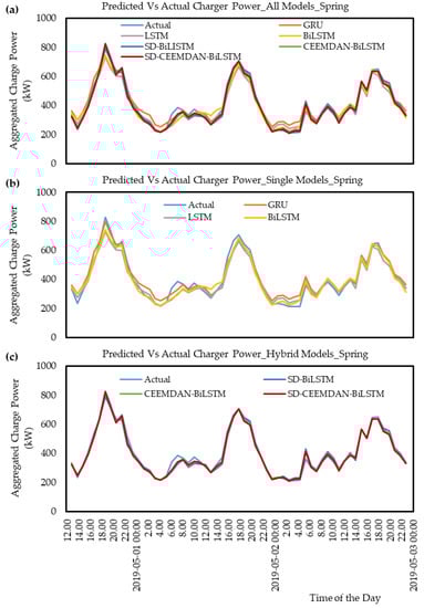
Figure 7.
Predictions and actual aggregated charge power during the three-day-ahead prediction period in spring for (a) all prediction models, (b) single prediction model, (c) hybrid prediction model.
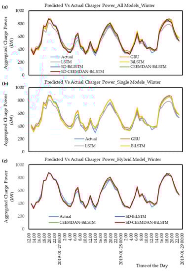
Figure 8.
Predictions and actual aggregated charge power during the three-day-ahead prediction period in winter for (a) all prediction models, (b) single prediction model, (c) hybrid prediction model.
The aggregated charge power (kW) in spring and winter are compared and the results show that the peak periods in spring are shorter than in winter, resulting in higher overall charge power in winter (Figure 7 and Figure 8). This might be due to decreased battery efficiency, a higher charging load for cabin heating, and more charging load per season in cold winter weather. Comparisons between the forecasting curve of the single models in spring and winter (Figure 7b and Figure 8b) show that the BiLSTM curves follow the actual data better than other models. Comparisons between the prediction curves of the hybrid models in spring and winter (Figure 7c and Figure 8c) show that the predicting curve of the proposed SD-CEEMDAN-BiLSTM model is closer to the original charge power curve than the other models.
Table 2 shows the error values of the six prediction models. The training period is from 20 August 2017 to 31 December 2018, and the prediction period is from 1 January 2019 to 30 May 2019. Among the six prediction models, the results obtained by using SD-CEEMDAN-BiLSTM are more fitted to the original data. The RMSE, MAPE, and MAE values are 14.5, 2.6, and 13.1, respectively, which are much smaller than other prediction models. These data indicate that the SD-CEEMDAN-BiLSTM model has better stability and accuracy and can be well applied to EV load prediction. LSTM has the maximum MAPE value. Although all three single models and other hybrid models followed the general trend of the raw data, their forecasting errors were high.
Table 2.
Prediction evaluation indicators for six models. MAE: Mean Absolute Error, MAPE: Mean Absolute Percent Error, RMSE: Root Mean Squared Error, GRU, LSTM, Bi-LSTM, SD-Bi-LSTM, CEEMDAN-Bi-LSTM, SD-CEEMDAN-Bi-LSTM.
Table 3 and Table 4 compare the MAPE values for all the models by month for the one-day-ahead and the three-day ahead prediction. The training period is from 20 August 2017 to 31 December 2018, and the prediction period is from 1 January 2019 to 30 May 2019. The results indicate that the proposed model is significantly superior to the single models and other hybrid models. MAPE of the SD-CEEMDAN-BiLSTM model is the lowest among all the models. The average forecasting accuracy of the proposed model reaches 97.93% and 97.29% in the one-day-ahead and the three-day-ahead prediction, respectively.
Table 3.
MAPE (%) of all the models per month for the one-day-ahead prediction.
Table 4.
MAPE (%) of all the models per month for the three-day-ahead prediction.
5. FutureWork
Issues that could be addressed in future work:
- Examine reinforcement learning approaches for dealing with real large datasets composed of time series.To learn the individual EV user energy consumption in order to reduce peak power on an aggregate level.To investigate the individual and cumulative impact of battery capacity and time of use rate on the charging behavior of EV users.
- Apply smart charging strategy to minimize overall vehicle energy use costs.
- Develop a methodology that facilitates the decision making in real-time, using models that can be applied to a wide range of vehicle models and/or groups.
6. Conclusions
This study proposes a hybrid model based on the SD selection, CEEMDAN signal processing technique, and the BiLSTM network. The proposed approach was compared with LSTM, GRU, SD-BiLSTM, and CEEMDAN-BiLSTM models to assess the effectiveness of the proposed model on hourly EV charging load forecasting. To achieve the best performance, fine-tuning and proper hyper-parameters were investigated. The performance of these prediction models was evaluated in terms of MAE, RMSE, and MAPE. The main conclusions of this study can be summarized as follows:
- 1.
- The hybrid approach is feasible and reasonable for the three-day-ahead load forecasting of a real-life dataset that was collected from 1000 EVs in nine provinces in Canada from 2017 to 2019.
- 2.
- The SD algorithm applied for optimizing the single models and the CEEMDAN technique applied in extracting the various components could both improve the prediction performance of the single models.
- 3.
- Overall, the proposed SD-CEEMDAN-BiLSTM model shows a competitive technique for enhancing the charging load prediction accuracy of the EV fleet.
Author Contributions
Conceptualization, A.M.; methodology, A.M.; software, A.M. and F.B.; formal analysis, A.M., E.E., and F.B.; investigation, A.M. and E.E.; writing—original draft preparation, A.M., E.E., and F.B.; writing—review and editing, A.M., E.E., and F.B. All authors have read and agreed to the published version of the manuscript.
Funding
This research is financially supported by Natural Resources Canada, the Program of Energy Research and Development under grant CEO-19-112.
Institutional Review Board Statement
Not applicable.
Informed Consent Statement
Not applicable.
Data Availability Statement
Data are contained within this review article.
Acknowledgments
The authors would like to thank the Office of Energy Research and Development (OERD) of Natural Resources Canada for their valuable financial support.
Conflicts of Interest
The authors declare no conflict of interest.
Nomenclature
| EV | Electric Vehicle |
| STLF | Short-Term Load Forecasting |
| SD | Similar Day |
| AI | Artificial Intelligence |
| ML | Machine Learning |
| RNN | Recurrent Neural Network |
| LSTM | Long Short-Term Memory |
| BiLSTM | Bidirectional LSTM |
| GRU | Gated Recurrent Unit |
| XGB | Extreme Gradient Boosting |
| EMD | Empirical Mode Decomposition |
| IMFs | Intrinsic Mode Functions |
| EEMD | Ensemble EMD |
| CEEMDAN | CEEMD with Adaptive Noise |
| MR | Mid-Range |
| SR | Short-Range |
| the nth decision tree | |
| F | space |
| loss function | |
| prediction and target values | |
| regularization term | |
| n | the number of targets |
| number of leaf nodes | |
| the score of leaf nodes | |
| γ and β | penalty factors |
| white noise | |
| original signal | |
| Si(t) | experimental signal |
| residual | |
| input gate | |
| forget gate | |
| output gate | |
| activation functions | |
| zt | update gate vector |
| Ht−1 | output at t−1 time slot |
| rt | reset gate vector |
| xt | input gate at the current moment |
| Ϭg, ϕh | sigmoid and hyperbolic function |
| Čt | the current state of the cell |
| cell state | |
| input, output, and update gates | |
| activation function and reset gate | |
| W, U, b | parameter matrices and vector |
| sigmoid and hyperbolic function | |
| total predicted number of days | |
| predictive value | |
| actual value | |
| test set | |
| final predicted result | |
| RMSE | root mean squared error |
| MAE | mean absolute error |
| MAPE | mean absolute percent error |
| MSE | mean squared error |
References
- World Economic Forum. Worldwide Sales of EVs. Available online: https://www.weforum.org/agenda/2022/02/electric-cars-sales-evs/ (accessed on 24 February 2022).
- PV magazine International. Global Electric Car Fleet by 2030. Available online: https://www.pv-magazine.com/2019/05/28/global-electric-car-fleet-may-reach-250-million-by-2030/ (accessed on 24 February 2022).
- Zhu, J.; Yang, Z.; Guo, Y.; Zhang, J.; Yang, H. Short-Term Load Forecasting for Electric Vehicle Charging Stations Based on Deep Learning Approaches. Appl. Sci. 2019, 9, 1723. [Google Scholar] [CrossRef]
- Xiao, L.; Shao, W.; Wang, C.; Zhang, K.; Lu, H. Research and Application of a Hybrid Model Based on Multi-Objective Optimization for Electrical Load Forecasting. Appl. Energy 2016, 180, 213–233. [Google Scholar] [CrossRef]
- Peng, T.; Zhang, C.; Zhou, J.; Nazir, M.S. An Integrated Framework of Bi-Directional Long-Short Term Memory (BiLSTM) Based on Sine Cosine Algorithm for Hourly Solar Radiation Forecasting. Energy 2021, 221, 119887. [Google Scholar] [CrossRef]
- Ma, Z.; Chen, H.; Wang, J.; Yang, X.; Yan, R.; Jia, J.; Xu, W. Application of Hybrid Model Based on Double Decomposition, Error Correction and Deep Learning in Short-Term Wind Speed Prediction. Energy Convers. Manag. 2020, 205, 112345. [Google Scholar] [CrossRef]
- Lin, H.; Sun, Q. Crude Oil Prices Forecasting: An Approach of Using CEEMDAN-Based Multi-Layer Gated Recurrent Unit Networks. Energies 2020, 13, 1543. [Google Scholar] [CrossRef]
- Lin, Y.; Yan, Y.; Xu, J.; Liao, Y.; Ma, F. Forecasting Stock Index Price Using the CEEMDAN-LSTM Model. N. Am. J. Econ. Financ. 2021, 57, 101421. [Google Scholar] [CrossRef]
- Zhou, J.; Chen, D. Carbon Price Forecasting Based on Improved CEEMDAN and Extreme Learning Machine Optimized by Sparrow Search Algorithm. Sustainability 2021, 13, 4896. [Google Scholar] [CrossRef]
- Massaoudi, M.; Refaat, S.S.; Chihi, I.; Trabelsi, M.; Oueslati, F.S.; Abu-Rub, H. A Novel Stacked Generalization Ensemble-Based Hybrid LGBM-XGB-MLP Model for Short-Term Load Forecasting. Energy 2021, 214, 118874. [Google Scholar] [CrossRef]
- Wu, J.; Zhou, T.; Li, T. Detecting Epileptic Seizures in EEG Signals with Complementary Ensemble Empirical Mode Decomposition and Extreme Gradient Boosting. Entropy 2020, 22, 140. [Google Scholar] [CrossRef]
- Zheng, H.; Yuan, J.; Chen, L. Short-Term Load Forecasting Using EMD-LSTM Neural Networks with a Xgboost Algorithm for Feature Importance Evaluation. Energies 2017, 10, 1168. [Google Scholar] [CrossRef]
- Zhu, K.; Geng, J.; Wang, K. A Hybrid Prediction Model Based on Pattern Sequence-Based Matching Method and Extreme Gradient Boosting for Holiday Load Forecasting. Electr. Power Syst. Res. 2021, 190, 106841. [Google Scholar] [CrossRef]
- Haq, R. Machine Learning for Load Profile Data Analytics and Short-Term Load Forecasting. Master’s Thesis, Electrical South Dakota State University, Brookings, SD, USA, 2019. [Google Scholar]
- Nie, H.; Liu, G.; Liu, X.; Wang, Y. Hybrid of ARIMA and SVMs for Short-Term Load Forecasting. Energy Procedia 2012, 16, 1455–1460. [Google Scholar] [CrossRef]
- Chen, Y.; Luh, P.B.; Guan, G.; Zhao, Y.; Michel, L.D.; Coolbeth, M.A.; Friedland, P.B.; Rourke, S.J. Short-Term Load Forecasting: Similar Day-Based Wavelet Neural Networks. IEEE Trans. Power Syst. 2010, 25, 322–330. [Google Scholar] [CrossRef]
- Henselmeyer, S.; Grzegorzek, M. Short-Term Load Forecasting Using an Attended Sequential Encoder-Stacked Decoder Model with Online Training. Appl. Sci. 2021, 11, 4927. [Google Scholar] [CrossRef]
- Sun, X.; Luh, P.B.; Cheung, K.W.; Guan, W.; Michel, L.D.; Venkata, S.S.; Miller, M.T. An Efficient Approach to Short-Term Load Forecasting at the Distribution Level. IEEE Trans. Power Syst. 2016, 31, 2526–2537. [Google Scholar] [CrossRef]
- Mamun, A.A.; Sohel, M.; Mohammad, N.; Haque Sunny, M.S.; Dipta, D.R.; Hossain, E. A Comprehensive Review of the Load Forecasting Techniques Using Single and Hybrid Predictive Models. IEEE Access 2020, 8, 134911–134939. [Google Scholar] [CrossRef]
- Bouktif, S.; Fiaz, A.; Ouni, A.; Serhani, M. Optimal Deep Learning LSTM Model for Electric Load Forecasting Using Feature Selection and Genetic Algorithm: Comparison with Machine Learning Approaches. Energies 2018, 11, 1636. [Google Scholar] [CrossRef]
- Kong, W.; Dong, Z.Y.; Jia, Y.; Hill, D.J.; Xu, Y.; Zhang, Y. Short-Term Residential Load Forecasting Based on LSTM Recurrent Neural Network. IEEE Trans. Smart Grid 2019, 10, 841–851. [Google Scholar] [CrossRef]
- Wu, L.; Kong, C.; Hao, X.; Chen, W. A Short-Term Load Forecasting Method Based on GRU-CNN Hybrid Neural Network Model. Math. Probl. Eng. 2020, 2020, 1428104. [Google Scholar] [CrossRef]
- Du, J.; Cheng, Y.; Zhou, Q.; Zhang, J.; Zhang, X.; Li, G. Power Load Forecasting Using BiLSTM-Attention. IOP Conf. Ser. Earth Environ. Sci. 2020, 440, 032115. [Google Scholar] [CrossRef]
- Huang, Z.; Yang, F.; Xu, F.; Song, X.; Tsui, K.-L. Convolutional Gated Recurrent Unit–Recurrent Neural Network for State-of-Charge Estimation of Lithium-Ion Batteries. IEEE Access 2019, 7, 93139–93149. [Google Scholar] [CrossRef]
- Mohsenimanesh, A.; Entchev, E.; Lapouchnian, A.; Ribberink, H. A Comparative Study of Deep Learning Approaches for Day-Ahead Load Forecasting of an Electric Car Fleet. In Database and Expert Systems Applications—DEXA 2021 Workshops; Kotsis, G., Tjoa, A.M., Khalil, I., Moser, B., Mashkoor, A., Sametinger, J., Fensel, A., Martinez-Gil, J., Fischer, L., Czech, G., et al., Eds.; Communications in Computer and Information Science; Springer International Publishing: Cham, Switzerland, 2021; Volume 1479, pp. 239–249. [Google Scholar] [CrossRef]
- AL-Musaylh, M.S.; Deo, R.C.; Li, Y.; Adamowski, J.F. Two-Phase Particle Swarm Optimized-Support Vector Regression Hybrid Model Integrated with Improved Empirical Mode Decomposition with Adaptive Noise for Multiple-Horizon Electricity Demand Forecasting. Appl. Energy 2018, 217, 422–439. [Google Scholar] [CrossRef]
- Hong, W.-C.; Fan, G.-F. Hybrid Empirical Mode Decomposition with Support Vector Regression Model for Short Term Load Forecasting. Energies 2019, 12, 1093. [Google Scholar] [CrossRef]
- Colominas, M.A.; Schlotthauer, G.; Torres, M.E. Improved Complete Ensemble EMD: A Suitable Tool for Biomedical Signal Processing. Biomed. Signal Process. Control 2014, 14, 19–29. [Google Scholar] [CrossRef]
- Rezaie-Balf, M.; Maleki, N.; Kim, S.; Ashrafian, A.; Babaie-Miri, F.; Kim, N.W.; Chung, I.-M.; Alaghmand, S. Forecasting Daily Solar Radiation Using CEEMDAN Decomposition-Based MARS Model Trained by Crow Search Algorithm. Energies 2019, 12, 1416. [Google Scholar] [CrossRef]
- Jiang, F.; Zhang, Y. Electric Load Forecasting Based on CEEMDAN and LSSVM Optimized by Cuckoo Search Algorithm. In Proceedings of the 2019 IEEE 3rd Conference on Energy Internet and Energy System Integration (EI2), Changsha, China, 8–10 November 2019; pp. 1536–1541. [Google Scholar] [CrossRef]
- Torres, M.E.; Colominas, M.A.; Schlotthauer, G.; Flandrin, P. A Complete Ensemble Empirical Mode Decomposition with Adaptive Noise. In Proceedings of the 2011 IEEE International Conference on Acoustics, Speech and Signal Processing (ICASSP), Prague, Czech Republic, 22–27 May 2011; pp. 4144–4147. [Google Scholar] [CrossRef]
- Zhu, J.; Yang, Z.; Mourshed, M.; Guo, Y.; Zhou, Y.; Chang, Y.; Wei, Y.; Feng, S. Electric Vehicle Charging Load Forecasting: A Comparative Study of Deep Learning Approaches. Energies 2019, 12, 2692. [Google Scholar] [CrossRef]
- Bidirectional Recurrent Neural Networks—Wikipedia. Available online: https://en.wikipedia.org/wiki/Bidirectional_recurrent_neural_networks (accessed on 23 June 2022).


Publisher’s Note: MDPI stays neutral with regard to jurisdictional claims in published maps and institutional affiliations. |
© 2022 by the authors. Licensee MDPI, Basel, Switzerland. This article is an open access article distributed under the terms and conditions of the Creative Commons Attribution (CC BY) license (https://creativecommons.org/licenses/by/4.0/).