Space Node Topology Optimization Design Considering Anisotropy of Additive Manufacturing

Featured Application

In this paper, the anisotropy of the mechanical properties of additively manufactured products was investigated. When carrying out a lightweight design, considering the anisotropy during manufacturing, it can provide accurate performance estimates for subsequent manufacturing. The research object of this paper was the space node, which is very suitable for lightweight design because of its complex force. However, this method can also be used for those products that need to consider the performance after manufacture, especially in mass production, whereby the most suitable molding direction can be found using this method.

Abstract

At present, a large number of scholars have conducted related research on topology optimization for additive manufacturing (AM). However, there are few relevant research reports on the impact of different directions of additive manufacturing on the optimal design and manufacturing results. In this paper, using the bidirectional evolutionary optimization (BESO) method, anisotropic optimization analysis was carried out on space nodes that are currently popular in the field of additive manufacturing and topology optimization. The elastic constants in different directions were used as anisotropic material properties for optimization research in this paper through tensile testing, which was carried out on 316L stainless-steel specimens fabricated using Selective Laser Melting (SLM) technology. In addition, SEM analyses were performed to explore the microscopic appearance of the material. The study found that additive manufacturing is affected by the printing direction in terms of both macroscopic mechanical properties and microscopic material structure; the deformation obtained by anisotropic optimization was about 1.1–2.3% smaller than that obtained by isotropic optimization.

1. Introduction

Topology optimization is the most advanced type of optimization, which can redistribute the material of the structure and distribute the material in the most reasonable position. This idea originated from the parameter optimization of Michell [1] trusses in 1904. Later, Bendsøe and Kikuchi [2] introduced topology optimization to the optimal design of continuum structures. Over the past few decades, with the continuous in-depth research on the optimization method of continuum structure, many topology optimization methods such as the solid isotropic material with penalization (SIMP) method [3], the BESO method [4], the independent continuous mapping (ICM) method [5], the moving morphable component (MMC) method [6], and the level set method (LSM) [7] have been created on this basis. It is favored by engineers in topology optimization for carrying out lightweight design and ensuring structural strength without relying on human design experience. The development of some methods such as evolutionary topology optimization (ETO) [8], floating projection topology optimization (FPTO) [9], and smooth-edged material distribution for optimizing topology (SEMDOT) [10] can generate a clear and smooth boundary representation. These methods break the limitation of the finite element mesh to enable researchers to get a relatively accurate model boundary. This can be considered a significant key for promoting topology optimization in engineering.

Additive manufacturing technology is well known in the form of 3D printing, which enables the direct fabrication of topologically optimized structures. Brackett et al. [11] pointed out that the biggest bottleneck of the application of typical topology optimization methods to additive manufacturing is that the additive manufacturing constraints are not considered. However, with the development of technologies, some researchers have found some methods to solve the problems where the overhanging part of the structure may collapse during manufacture, and topology results are not smooth. For example, Langelaar [12] developed an AM filter to overcome the overhanging angle problem by combining a layer-wise nonlinear spatial filtering scheme using the SIMP method. Gaynor and Johnson et al. [13] developed a sub-support method for cone density filtering based on the SIMP method. Both methods have been used in commercial software. In recent years, YunFei Fu et al. developed a new SIMP-based method by integrating Langelaar’s AM filter, which is capable of generating smooth boundaries [14]. In addition, YunFei Fu et al. thoroughly investigated the influences of parameters including the filter radius, mesh size, and target volume fraction on the performance and manufacturability of smooth self-supporting topologies [15]. Importantly, these methods have been validated in practical manufacturing, and the manufacturing of topology optimization results is no longer affected by the shape of complex structures. These advanced studies have brought AM and topology optimization closer together. Although topology optimization and additive manufacturing have only been used in fields with high-precision requirements such as high-end equipment and aerospace for a long time [16], with the advancement of additive manufacturing technology and the in-depth study of topology optimization design, many researchers have turned their attention to other industrial designs that can combine topology optimization and additive manufacturing.

As a prefabricated building, space structure is one of the application directions of additive manufacturing and topology optimization. It is important for the nodes to be stronger than the rods in the space structure; otherwise, the damage to nodes will cause extensive collapse as they are connected with many rods. In addition to being lightweight, topology-optimized space nodes will have greater stiffness, meeting this requirement. Zhao et al. [17,18] carried out topology optimization of maximum stiffness and minimum mass for cable-rod nodes in space structures. Wang [19] studied the optimization and additive manufacturing of bifurcated cast steel joints. Liu [20] took the spherical node as the research object and compared the mechanical properties of multi-objective optimization and single-objective optimization. Seifi [21] used the over-section method and the BESO method to study the topology optimization design of a six-bar box node in Sunshine Valley. These studies have greatly broadened the application scope of additive manufacturing and topology optimization, as well as accelerated the continuous innovation of manufacturing technology and industrial applications.

It should be noted that it is also necessary to consider the anisotropy problem caused by additive manufacturing in the application research of topology optimization for additive manufacturing, concerning components that require stiffness, especially space nodes with complex forces. The general topology optimization only considers isotropic materials, which ignores the anisotropy caused by the manufacturing process. Numerous articles have pointed out that anisotropy is common when most materials are used in additive manufacturing, where the mechanical properties of the manufactured components are almost different in all directions. Song [22] conducted tensile and compression tests in different directions on specimens made of PLA, which showed strong anisotropy in the test. In addition to PLA materials, AM specimens of other polymer materials, such as ABS [23], polypropylene [24], and polycarbonate [25], also showed anisotropy in the experiments. With regard to the anisotropy of metal materials, researchers have mainly studied 316L stainless steel. Alsalla [26], Zhou [27], and Dong [28] studied 316L stainless-steel specimens prepared by selective laser melting. Studies found that the metal specimens also had anisotropy, with the mechanical properties in the manufacturing direction being the weakest. The microstructure of the samples also showed grains with directional characteristics. Furthermore, the same was true in terms of microstructure. Ntintakis’s [29] studies on topologically optimized microstructures showed that the additive manufacturing of microstructures also has anisotropic behavior. Rastegarzadeh [30] proposed a gradient-based algorithm to simultaneously optimize the microscale structures and macroscale material properties, and the high computational efficiency and superior structural mechanical properties of the orthotropic porous material were experimentally demonstrated. Therefore, it is necessary to consider the anisotropy caused by the manufacturing process in the optimization and manufacturing process.

Using the Abaqus solver and Matlab programming, this paper integrated an optimization platform for topology optimization and conducted an additive manufacturing mechanical test with 316L stainless steel as the research object to study the mechanical properties of the material in different directions. The elastic constants in different directions obtained from the experiment were used as anisotropic material properties for optimization research. In the optimization analysis, the anisotropic parameters are respectively substituted into the model optimized by the isotropic parameters for calculation, to analyze the mechanical properties of the isotropically optimized nodes in different directions during manufacture. In addition, unlike the general isotropic study, this paper also input the anisotropic parameters before topology optimization. This generated the best results for different manufacturing directions, enabling a comparison with isotropic optimization results and an exploration of how adding anisotropic parameters affects topology optimization. The conclusions obtained in this paper can provide a reference for the practical application of additive manufacturing and increase the applicability of topology optimization design.

2. Materials and Methods

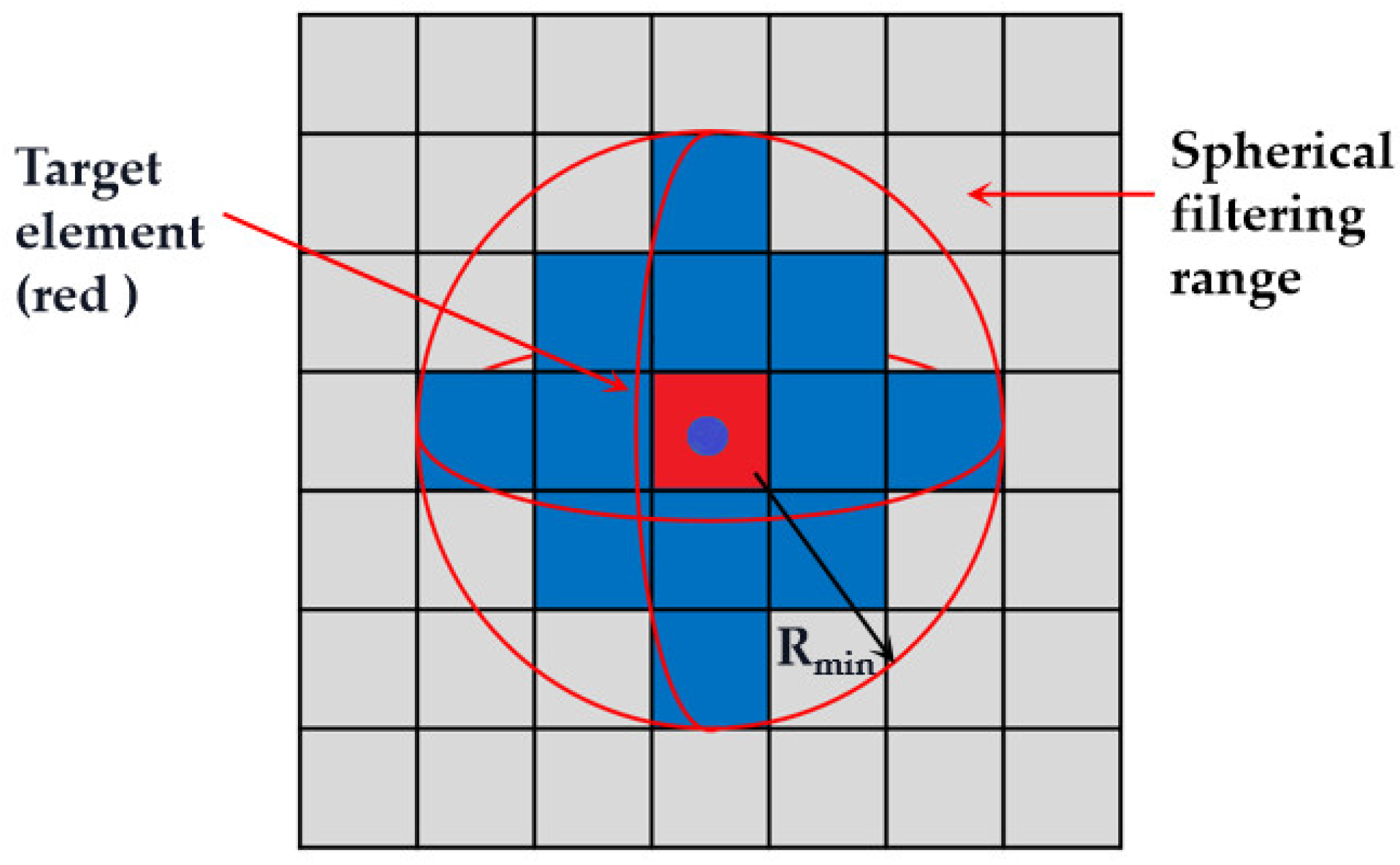
2.1. Secondary Development of the BESO Method

The BESO method is one of the most popular topology optimization methods of continuum structures. BESO is optimized by continuously reducing the volume, which can avoid falling into the local optimal solution, with broad prospects for secondary development.

Compliance is usually taken as the objective function when optimizing the space nodes that require stronger stiffness, and optimizing the structural shape with the smallest deformation while taking into account the lightweight design. This paper uses the BESO method based on the finite element method, which can ensure the efficiency and effect of the optimization, using the equal-volume regular hexahedron square as the variable element to get the energy density of the element as the design variable.

Its mathematical description is as follows:

$$\{\begin{array}{ll}Minimize:& \mathrm{C}\left(X_i\right)=F^{\mathrm{T}}U\\ \mathrm{s}.\mathrm{t}.:& V^{*}-{\displaystyle \sum _i^n}{V}_i=0\\ & X_i=1 wheni\in {\mathsf{\Omega }}_1\\ & X_i=x_{min}wheni\in {\mathsf{\Omega }}_0\end{array},$$

(1)

where C is the compliance, F is the force matrix, U is the displacement (deformation) matrix, V* is the target volume fraction, V_i is the volume of the i-th element, X_i is the design variable of the i-th element, n is the total number of solid elements, x_min is a nonzero minimum value, Ω₁ is the solid region, and Ω₀ is the hole region.

The formula takes compliance C as the objective function and strives to minimize the compliance, which means that the deformation U is the smallest when the load F is unchanged, and the structural configuration at V* volume is obtained, so as to achieve lightweight and maximize stiffness. When i belongs to the solid area, the design variable X_i is itself; when i belongs to the hole area, it is necessary to carry out the X_i penalty. This is to make it approximate to air, but not exactly equal to 0, to avoid matrix singularity [31].

To make the results continuous in the finite element calculation, the most commonly used BESO method introduces the material interpolation formula of the SIMP method. The material interpolation method can make the hole area unit get the sensitivity penalty in the iterative calculation, and then effectively distinguish the solid unit and the hole area unit.

$$\mathrm{E}(x_i)=x_i^p{\mathrm{E}}_1,$$

(2)

where E₁ denotes the Young’s modulus of the solid material, x_i is the design variable of the i-th element, and p is the penalty exponent.

After the model is calculated by finite element software, the energy density of each element is obtained. Generally, the large value is not corrected, but the material method is used to penalize the value of the element in the hole area to reduce the weight of sensitivity filtering.

This paper adopts a solid-void design; hence, according to the relevant literature, it can be expressed by the following formula [32]:

$$\frac{\partial C}{\partial x_i}=-\frac{p{x}_i^{p-1}}{2}{U}_i^T{K}_i{U}_i,$$

(3)

where K_i is the elemental stiffness matrix.

The design variable is discrete because materials in solid and void are different, and every design variable of the individual element is represented by a sensitivity, thereby the formula can be defined by:

$${\alpha }_i=-\frac{1}{p}\frac{\partial C}{\partial x_i}=\{\begin{array}{ll}\frac{1}{2}{U}_i^{\mathrm{T}}{K}_i{U}_i& when{x}_i=1\\ \frac{x_{min}^{p-1}}{2}{U}_i^{\mathrm{T}}{K}_i{U}_i& when{x}_i=x_{\min }\end{array}$$

(4)

Then the sensitivity number will decline to nearly 0 with the penalty exponent increasing to infinity.

In general, when using an optimization program based on finite element software, it cannot be calculated to define a void region material as zero; therefore, the void material is defined as a material with lower performance. In this way, two materials need to be defined in the optimization, and the formula is defined as

$${\alpha }_i=\{\begin{array}{ll}\frac{1}{2}[1-\frac{{\mathrm{E}}_2}{{\mathrm{E}}_1}]U_i^{\mathrm{T}}{K}_i^1{U}_i& \mathrm{for}\mathrm{solid}\mathrm{area}\\ \frac{1}{2}[\frac{x_{min}^{p-1}({\mathrm{E}}_1-{\mathrm{E}}_2)}{x_{min}^p{\mathrm{E}}_1+(1-x_{min}^p){\mathrm{E}}_2}]U_i^{\mathrm{T}}{K}_i^2{U}_i& \mathrm{for}\mathrm{hole}\mathrm{area}\end{array},$$

(5)

which can be simplified as

$${\alpha }_i=\{\begin{array}{ll}\frac{1}{2}[1-\frac{{\mathrm{E}}_2}{{\mathrm{E}}_1}]U_i^{\mathrm{T}}{K}_i^1{U}_i& \mathrm{for}\mathrm{solid}\mathrm{area}\\ 0& \mathrm{for}\mathrm{hole}\mathrm{area}\end{array},$$

(6)

where α is the element sensitivity, E₁ and E₂ are the element elastic moduli of the solid area and the hole area, respectively, K is the stiffness matrix calculated from the elastic moduli E₁ and E₂, and P is the penalty index, whose increase will decrease the sensitivity α, thus achieving the effect of increasing the penalty.

According to the material interpolation method described above, the elements in the hole area are assigned a sensitivity value that is approximate and not equal to 0, while the element’s sensitivity in the solid area receives the appropriate adjustments.

A sensitivity filter needs to be added because the structure cannot be kept smooth. Although the use of the material interpolation method enables the elements to better participate in the iterative calculation, island elements are prone to appear adjacent to the solid element and the hole area element.

Figure 1 is a schematic diagram of the sensitivity filter. The sensitivity filtering method is introduced to solve the checkerboard effect caused by the discontinuity of the grid sensitivity of the elements. A spherical filter is usually used in the three-dimensional optimization algorithm, which can ensure the smoothness of the structure after filtering. In the figure, the blue elements are the elements involved in filtering, and these elements are all within the scope of the sphere. By processing the elements within a certain radius Rmin near the target element according to the distance weighted average, the grid becomes stable and continuous. In this way, even element values with large differences can be made continuous.

The weights are calculated as follows [33]:

$$\begin{array}{c}\omega (r_j)=r_{min}-r_j\\ j=1,2\dots m\end{array}$$

(7)

where r_min is the filtering range, r_j is the distance between unit j and the target unit, and m is the number of units within the range of r_min.

The unit sensitivity is calculated according to the following formula [33]:

$$\begin{array}{l}{a}_i=\frac{{\displaystyle \sum _{j=1}^n{a}_j^n\omega (r_j)}}{{\displaystyle \sum _{j=1}^n\omega (r_j)}}\\ i=1,2,\dots n;j=1,2,\dots m\end{array}$$

(8)

where i represents the serial number of the target unit, and j represents the serial number of the unit participating in the filtering within the filtering range. As the iterative process progresses, the boundaries of soft and solid elements become smooth. The sensitivity filtering method not only solves the checkerboard problem but also effectively reduces the dependence on the grid, which is one of the cores of the topology optimization method.

Lastly, the solid elements and the pore elements are divided according to the volume fraction using the bisection method. This step requires finding a critical value that distinguishes solid elements from hole area elements. The maximum and minimum sensitivities of all units are summed before taking the average. When using this average as the critical value, if the number of solid elements is greater than the volume constraint, the average is again averaged with the maximum value. Otherwise, the average is summed with the minimum value. In the recycling process, the most accurate critical value is obtained by continuous approximation through the bisection method, to carry out the unit division.

The formula is as follows [34]:

$$\{\begin{array}{l}{a}_{th}=\frac{a_{min}+a_{max}}{2}\\ a_{th}=\frac{a_{th}+a_{max}}{2}\mathrm{if}V>V_{goal}\\ a_{th}=\frac{a_{th}+a_{min}}{2}\mathrm{if}V<V_{goal}\end{array},$$

(9)

where a_th is the critical value of the division unit, a_min is the minimum sensitivity, a_max is the maximum sensitivity, V is the current volume value, and V_goal is the target volume under the control of the current evolution rate.

With a certain number of optimization iterations, the convergence of the algorithm iteration is judged according to the historical change of sensitivity.

The formula is as follows [31,32,33]:

$$\frac{\left|{\displaystyle \sum _{i=1}^N{C}_{K-i+1}-{\displaystyle \sum _{i=1}^N{C}_{K-i-N+1}}}\right|}{{\displaystyle \sum _{i=1}^N{C}_{K-i+1}}}\le e,$$

(10)

where C is the compliance of each iteration, K is the iteration order, and N is a positive integer. When it is smaller than the relative error e, it is judged to be converged.

On the basis of the above optimization theory, the algorithm flow of secondary development is shown in Figure 2:

When using this method, the finite element analysis model is first established and meshed in Abaqus. Then, the .inp format of the Abaqus calculation file is exported.

Then, the DOS command ‘dos(strcat(‘abaqus job=‘,Name,’ double interactive cpus=2’))’ based on Matlab programming is called, the finite element .inp file is calculated in the background, and the .ODB result file is obtained.

The resulting data from the .ODB file are then extracted by calling a Python program, which contains the stress and energy of the element. The extraction method is to open the .ODB file through the openOdb() command in python, and to accurately extract the target SET’s data with the help of the command ‘odb.steps[].frames[].fieldOutputs[].getSubset(region=odb.rootAssembly.instances.elementSets)’, because python tools have a rich database to call.

When analyzing, the material properties, penalty index, evolution rate, unit range, and filter radius are firstly set. In Matlab, according to the arrangement of elements of the finite element model, the element values obtained from .odb are correspondingly arranged into a three-dimensional matrix. Sensitivity analysis and filtering are then performed. Lastly, on the basis of the filtered design variables, the unit is divided using the bisection method, and a new .inp file is written in Matlab through the ‘fopen’ and ‘fprintf’ commands. On the basis of the set evolution rate, the volume is continuously reduced until the target volume fraction is reached. This can be achieved with the help of 3D modeling software and a 3D printer.

This completes the optimization, followed by actinic processing and additive manufacturing.

Relying on mature commercial finite element solvers, this method has good reliability and can be easily invoked when solving optimization problems.

2.2. 316L Stainless-Steel Anisotropy and Microscopic Research

To obtain the anisotropic mechanical properties of 316L stainless-steel components manufactured using SLM technology, this paper printed small-sized samples based on the ASTM-E8 specification, conducted tensile tests, and studied the mechanical properties in each molding direction. The morphological changes of the samples before and after stretching were analyzed by SEM, and the failure mechanism was explored.

The tensile properties of the specimen were determined according to the ASTM-E8 metal tensile test specification, which is a dumbbell-shaped specimen, as shown in Figure 3, and the specific dimensions are shown in

Table 1. Parameters of 316L stainless-steel sample.

Name	Length (mm)
Gauge length G	25
Clamping section width C	10
Clamping part length B	30
Total length L	100
Width W	6
Thickness T	6
Radius R	6

.

In order to compare the influence of the mechanical properties of the 316L stainless-steel printed parts in all directions, the test pieces in this paper were printed in three orientations: vertical, side, and flat. The scanning path direction and printing direction of the samples manufactured in this paper are shown in Figure 4.

The coding of the sample in Figure 4 indicates the plane on which the largest surface of the sample is located. For example, the largest surface of the vertically printed sample is in the ZX plane in Figure 4; hence, ZX is used to represent vertical printing.

There was a difference between vertical and flat printing. When the vertically printed sample was stressed, the bonding of each layer of the printed surface was relatively weak, which affected the tensile properties. For the flat-printed style, the performance in this direction was best since the direction of the tensile test was the direction of the scanning path and stretched along the grain. Side-printed samples also performed better in tensile tests than those printed vertically. However, the side-printed samples did not stretch according to the scanning path during the tensile test; hence, the mechanical properties were weak. In general, the mechanical properties of the flat-printed samples should be the strongest, and the vertical-printed samples should be the weakest.

The parameters of 316L stainless-steel material are shown in

Table 2. The stainless-steel metal powder parameters.

Physical properties	Particle size (μm)	Shape	Hall flowmeter (s)	Loose packing density (cm3)
	15–53	Ball type	40	3.9
Elemental composition	Fe	S	Cr	P
	margin	≤0.03%	16–18%	≤0.0045%
	Ni	Mo	Mn	C
	10–14%	2–3%	≤2%	0.03%

, and the sample printing process parameters are shown in

Table 3. The 316L stainless-steel sample printing process information.

Print Direction	Powder Thickness (mm)	Scan Speed (mm/s)	Laser Power (W)
Side	0.035	1800	286
Flat	0.035	1800	286
Vertical	0.035	1800	286

.

In order to ensure that the performance comparison of the specimens was valid, all printed specimens were manufactured and printed under the same process parameters.

In this paper, the failure of the sample before and after the tensile test was observed, and the difference in the internal structure of the sample was observed through SEM analysis. The results are compared in Section 3.3.

2.3. Effects of Anisotropy on Node Optimization

Additive manufacturing is based on its stacked manufacturing method; thus, it can be regarded as a composite sheet, and the material elastic constant obtained from the tensile test is added as a material property. The tensile test results of different manufacturing directions can be approximately regarded as the properties of the direction. By changing the elastic constant, the printing direction of the model is defined in the algorithm. As shown in Figure 5, there will be different mechanical properties in different three directions in any layer which taken out from the printed part (small cube). It can be represented by the mechanical properties of flat, vertical, and side printed samples.

Shear modulus is expressed as follows according to [35]:

$$\mathrm{G}=\frac{\mathrm{E}}{2(1+\mathsf{\nu })},\mathrm{E}>0,\mathrm{G}>0,$$

(11)

where E is the elastic modulus, ν is the Poisson’s ratio, and G is the shear modulus.

3. Results

3.1. Optimization of Space Nodes

To highlight the stress complexity of the optimized nodes and to show the robustness of the secondary development algorithm, this paper chose to use ideal cube nodes [17,18,31] under combined tension and shear load as a calculation example. The size of the cube design domain was 80 mm × 80 mm × 80 mm. As shown in Figure 6, one end of the node was fixed, and the other three ends were subjected to axial tension and vertical shear. The shear force was 10,000 N, and the axial force was applied using a pressure of 500 Pa.

The sample was defined as an isotropic material with an elastic modulus of 2.06 × 105 MPa and a density of 7.85 g/cm³. The calculation results are shown in Figure 7. With further iterations, the target volume was reached at the 12th step, and the stress after the final convergence is shown below, highlighting its overall uniform distribution. As a result, there were fewer low-stress areas, with an overall state of high stress.

Therefore, the BESO secondary development procedure was reasonably reliable.

3.2. The 316L Stainless-Steel Tensile Test Results

As shown in Figure 8, the instrument used for the tensile test was the German Zwick electronic universal testing machine. Tensile tests were performed on nine samples in turn. The speed used in this test was 2 mm/min.

The measured stress–strain curve is shown in Figure 9:

It can be seen from Figure 9a–c that the tensile properties of the samples were similar in the same printing direction. This shows that the additive manufacturing technology had good stability, in addition to providing stable support for the research of anisotropic topology optimization based on its process.

The obtained data in each direction are shown in Figure 10.

According to Figure 10, the yield strength, elastic modulus, tensile strength, and elongation of flat printing were stronger compared to other layouts, while the results of vertical printing were the lowest. This result is consistent with the previous conclusions of other researchers [26,27], suggesting that the experimental data are reasonable.

3.3. SEM Microscopic Analysis

Figure 11 shows the observation pictures at 200× and 1000× magnification. The flat-printed samples performed well, showing uniform melting and fewer surface defects. The vertically printed samples had many pores, with mixed powders, poor quality, and unmelted metal powder. Such defects are often the main cause of stress concentration and will cause catastrophic damage. This situation may be due to two reasons: shrinkage defects caused by too fast cooling during manufacture or incomplete melting caused by fast scanning speed.

Figure 12 is a surface photograph of stretching results in different manufacturing directions. As shown in the figure, both samples had a well-shaped fracture path when fractured. In addition, at 200× magnification, it can be seen that both had unmelted metal powder but the melting quality of the flat-printed sample was significantly better. At the same time, it can be seen that the cracks of the flat-printed sample were small at 1000× magnification, while the vertical printing led to greatly expanded cracks on the surface of the sample, with a loose sliding phenomenon.

In Figure 13, it can be seen that the powder particles with a large number of second-phase particles at the fracture were not melted and showed a lot of dimples at 2000× magnification. The dimples were significantly denser and smaller under vertical printing. In terms of materials [36], the appearance of dimples was caused by the plastic deformation of the structure, with larger dimples indicating better ductility. The elongation of the vertically printed samples was lower than that of the flat-printed samples with larger dimples. At the same time, the large pores could also cause stress concentration, resulting in the vertically printed samples being more easily damaged during the test.

3.4. Anisotropic Optimization Analysis of Space Nodes

According to the above test data, the six elastic constant setting parameters shown in

Table 4. Elastic constant.

Printing Direction	Scan Direction	E1 (MPa)	E2 (MPa)	E3 (MPa)	G12 (MPa)	G13 (MPa)	G23 (MPa)
X	Y	1.26 × 105	1.66 × 105	1.58 × 105	60,769	63,846	48,462
X	Z	1.26 × 105	1.58 × 105	1.66 × 105	63,846	60,769	48,462
Y	X	1.66 × 105	1.26 × 105	1.58 × 105	60,769	48,462	63,846
Y	Z	1.58 × 105	1.26 × 105	1.66 × 105	63,846	48,462	60,769
Z	X	1.66 × 105	1.58 × 105	1.26 × 105	48,462	60,769	63,846
Z	Y	1.58 × 105	1.66 × 105	1.26 × 105	48,462	63,846	60,769

could be obtained [35].

The nodal conditions were kept consistent, and the material properties of the engineering elastic constants were set in the finite element calculation software to define the application direction of the parameters. The calculation file of the model was called in Matlab for analysis.

3.4.1. Anisotropic Analysis of Optimization Results for Isotropic Materials

In this Section, the optimization results of the isotropic materials in Section 3.1 are re-analyzed, the six parameters in Table 4 are substituted as engineering elastic constants, and the deformation analysis is carried out in Abaqus.

The analysis results in all directions are shown in Figure 14.

Figure 14 shows the effect of anisotropy during actual manufacturing, which was relatively large. It can be seen in the displacement cloud map that the node deformation of the Y-direction print with Z-scan was the smallest. In addition, the deformation of the node printed in the Z direction of this node was significantly larger than that of the other two directions. The difference between the maximum deformation and the minimum deformation was about 21.4%; hence, the anisotropy problem of additive manufacturing could not be ignored.

3.4.2. Anisotropic Optimization of Space Nodes

In addition to optimization with isotropic materials, this section performed topology optimization on nodes that incorporated anisotropic materials. Before optimization, the anisotropy parameters were taken as material properties and substituted into the space node model in Section 3.1 for optimization to compare the similarities and differences in optimization with and without taking into account anisotropy.

The results are shown in Figure 15.

As shown in Figure 15, the topology optimization of anisotropic materials resulted in quite differently shaped nodes compared to the results of isotropic optimization. In the X printing direction, since the force in the X direction was the largest but the material was the weakest when scanning in the Z direction, the shear modulus became weaker, and the shear force was affected, generating more hole areas. Compared with the results when scanning in the Y direction, larger holes also appeared in the center of the node. When printing in the Y direction and the Z direction, the difference between different scanning directions was small, but it can be seen that the shape was different. During Y-direction printing, due to the weak material properties in the Y-direction, more material accumulated on the boundary of the fixed end to provide more structural stiffness. When printing in the Z direction, the difference in the scanning direction resulted in the two sides being significantly affected by the shear force, while X-direction scanning weakened the shear stiffness on both sides of the node. Therefore, there was a little more material buildup at the boundary relative to the Y direction.

As shown in Figure 16, in the cases of isotropic optimization and anisotropic optimization, there was an optimal manufacturing solution for this node, i.e., printing in the Y direction and scanning in the Z direction. In this paper, the optimal manufacturing direction was shown at the blue flower, where the maximum deformation after optimization of the two was closest. However, in other directions, the optimization results considering the anisotropic parameters performed better than the isotropic optimization. In summary, it is necessary to take the manufacturing direction into account when optimizing space nodes that require greater stiffness.

4. Conclusions

This study was based on numerous previous studies by other researchers, and it integrated an optimization platform for topology optimization considering the anisotropy of AM. The anisotropy test and SEM analysis were carried out on the additive manufacturing samples in different printing directions, and the obtained anisotropy parameters were substituted into the optimization analysis. The following conclusions could be drawn:

(1)

By testing 316L stainless-steel products of SLM manufacturing technology, it was found that the mechanical properties of the printing direction were the weakest.

(2)

Under electron microscopy observation, there were more dimples and second-phase particles at the fracture of the sample stretched along the printing direction, which may have been due to incomplete powder melting caused by the interval of scanning speed between layers.

(3)

The attribute parameters of the forming direction had a significant influence on the optimized stiffness and optimized shape of the structure. In the case of the node in this paper, when adding parameters in various directions for analysis, both had the same direction most beneficial to actual manufacturing.

(4)

The deformation obtained by anisotropic optimization was about 1.09–2.19% smaller than that obtained by isotropic optimization. Therefore, when topology optimization is combined with additive manufacturing, it is necessary to consider the performance difference caused by the printing orientation.

References

1. Michell, A. The limits of economy of materials in frame structures. Philos. Mag. 1904, 8, 589–597. [Google Scholar] [CrossRef]
2. Bendsøe, M.P.; Kikuchi, N. Generating optimal topologies in structural design using a homogenization method. Comput. Methods Appl. Mech. Eng. 1988, 71, 197–224. [Google Scholar] [CrossRef]
3. Bendsøe, M.P.; Sigmund, O. Material interpolation schemes in topology optimization. Arch. Appl. Mech. 1999, 69, 635–654. [Google Scholar] [CrossRef]
4. Querin, O.M.; Steven, G.P.; Xie, Y.M. Evolutionary structural optimization (ESO) using a bidirectional algorithm. Eng. Comput. 1998, 15, 1031–1048. [Google Scholar] [CrossRef]
5. Sui, Y. A new method for structural topological optimization based on the concept of independent continuous variables and smooth model. Acta Mech. Sin. 1998, 14, 179–185. [Google Scholar] [CrossRef]
6. Guo, X.; Zhang, W.; Zhong, W. Doing Topology Optimization Explicitly and Geometrically—A New Moving Morphable Components Based Framework. J. Appl. Mech. 2014, 81, 081009. [Google Scholar] [CrossRef]
7. Rong, J. An Improved Level Set Method for Structural Topology Optimization. Acta Mech. Sin. 2007, 39, 8. [Google Scholar] [CrossRef]
8. Da, D.; Xia, L.; Li, G.; Huang, X. Evolutionary topology optimization of continuum structures with smooth boundary representation. Struct. Multidisc. Optim. 2018, 57, 2143–2159. [Google Scholar] [CrossRef]
9. Huang, X. On smooth or 0/1 designs of the fixed-mesh element-based topology optimization. Adv. Eng. Softw. 2021, 151, 102942. [Google Scholar] [CrossRef]
10. Fu, Y.F.; Rolfe, B.; Chiu, L.N.S.; Wang, Y.; Huang, X.; Ghabraie, K. SEMDOT: Smooth-edged material distribution for optimizing topology algorithm. Adv. Eng. Softw. 2020, 150, 102921. [Google Scholar] [CrossRef]
11. Brackett, D.; Ashcroft, I.; Hague, R. Topology optimization for additive manufacturing. In Proceedings of the 22nd Solid Freeform Fabrication Symposium, Austin, TX, USA, 8–10 August 2011; pp. 348–362. [Google Scholar]
12. Langelaar, M. Topology optimization of 3D self-supporting structures for additive manufacturing. Addit. Manuf. 2016, 12, 60–70. [Google Scholar] [CrossRef]
13. Gaynor, A.T.; Meisel, N.A.; Williams, C.B.; Guest, J.K. Topology optimization for additive manufacturing: Considering maximum overhang constraint. In Proceedings of the 15th AIAA/ISSMO Multidisciplinary Analysis & Optimization Conference, Atlanta, GA, USA, 16–20 June 2014. [Google Scholar]
14. Fu, Y.F.; Bernard, R.; Louis, N.S.C.; Wang, Y.; Huang, X.; Kazem, G. Design and experimental validation of self-supporting topologies for additive manufacturing. Virtual Phys. Prototyp. 2019, 14, 382–394. [Google Scholar] [CrossRef]
15. Fu, Y.F.; Bernard, R.; Louis, N.S.C.; Wang, Y.; Huang, X.; Kazem, G. Parametric studies and manufacturability experiments on smooth self-supporting topologies. Virtual Phys. Prototyp. 2020, 15, 22–34. [Google Scholar] [CrossRef]
16. Zhu, J.; Zhou, H.; Wang, C.; Zhou, L.; Yuan, S.Q.; Zhang, W.H. Development status and future of topology optimization technology for additive manufacturing. Aeronaut. Manuf. Technol. 2020, 63, 24–38. [Google Scholar]
17. Zhao, Y.; Chen, M.C.; Wang, Z. Topological optimization design of cable-rod structure nodes for additive manufacturing. J. Build. Struct. 2019, 40, 58–68. [Google Scholar]
18. Chen, M.C.; Zhao, Y.; Xie, Y.M. Topology optimization and additive manufacturing of spatial structure nodes. Chin. J. Civ. Eng. 2019, 52, 1–10. [Google Scholar]
19. Wang, L.X.; Du, W.F.; Zhang, F.; Zhang, H.; Gao, B.Q.; Dong, S.L. Topology optimization and 3D printing manufacturing of four-forked cast steel nodes. J. Build. Struct. 2021, 42, 37–49. [Google Scholar]
20. Liu, J.; Zhu, N.; Chen, L.; Liu, X. Structural Multi-objective Topology Optimization in the Design and Additive Manufacturing of Spatial Structure Joints. Int. J. Steel Struct. 2022, 22, 649–668. [Google Scholar] [CrossRef]
21. Hamed, S.; Anooshe, R.J.; Xu, S.Q.; Zhao, Y.; Xie, Y.M. Design optimization and additive manufacturing of nodes in gridshell structures. Eng. Struct. 2018, 160, 161–170. [Google Scholar] [CrossRef]
22. Song, Y.; Li, Y.; Song, W.; Yee, K.; Lee, K.-Y.; Tagarielli, V.L. Measurements of the mechanical response of unidirectional 3D-printed PLA. Mater. Des. 2017, 123, 154–164. [Google Scholar] [CrossRef]
23. Zhou, W.; Rezayat, H.; Siriruk, A.; Penumadu, D.; Babu, S.S. Structure-mechanical property relationship in fused deposition modelling. Mater. Sci. Technol. 2015, 31, 895–903. [Google Scholar]
24. Carneiro, O.S.; Silva, A.F.; Gomes, R. Fused deposition modeling with polypropylene. Mater. Des. 2015, 83, 768–776. [Google Scholar] [CrossRef]
25. Hill, N.; Haghi, M. Deposition direction-dependent failure criteria for fused deposition modeling polycarbonate. Rapid Prototyp. J. 2014, 20, 221–227. [Google Scholar] [CrossRef]
26. Alsalla, H.H.; Smith, C.; Liang, H. Effect of build orientation on the surface quality, microstructure and mechanical properties of selective laser melting 316L stainless steel. Rapid Prototyp. J. 2018, 24, 9–17. [Google Scholar] [CrossRef]
27. Zhou, Y.C.; Zhao, Y. Tensile properties of 316L stainless steel prepared by additive manufacturing technology. J. Civ. Eng. 2020, 53, 26–35. [Google Scholar]
28. Dong, Z.H.; Zheng, Z.J.; Peng, L. Effect of heat treatment on microstructure anisotropy of additively manufactured 316L stainless steel. Met. Heat Treat. 2021, 46, 45–52. [Google Scholar]
29. Ntintakis, I.; Stavroulakis, G.E. Infill Microstructures for Additive Manufacturing. Appl. Sci. 2022, 12, 7386. [Google Scholar] [CrossRef]
30. Rastegarzadeh, S.; Wang, J.; Huang, J. Two-Scale Topology Optimization with Isotropic and Orthotropic Microstructures. Designs 2022, 6, 73. [Google Scholar] [CrossRef]
31. Wang, X.J.; Zhang, X.A. Multiphase material layout and material/structure integration design. Acta Solid Mech. 2014, 35, 341–346. [Google Scholar]
32. Huang, X.; Xie, Y.M. Bi-directional evolutionary topology optimization of continuum structures with one or multiple materials. Comput. Mech. 2009, 43, 393. [Google Scholar] [CrossRef]
33. Yan, X.L.; Chen, J.W.; Hua, H.Y.; Zhang, Y.; Huang, X.D. Smooth topological design of structures with minimum length scale and chamfer/round controls. Comput. Methods Appl. Mech. Eng. 2021, 383, 113939. [Google Scholar] [CrossRef]
34. Wang, X.J.; Zhang, F.; Zhao, Y.; Wang, Z.Y.; Zhou, G.G. Research on 3D-Print Design Method of Spatial Node Topology Optimization Based on Improved Material Interpolation. Materials 2022, 15, 3874. [Google Scholar] [CrossRef] [PubMed]
35. Shen, G.L.; Hu, G.K.; Liu, B. Mechanics of Composite Materials, 2nd ed.; Tsinghua University Press: Beijing, China, 2013; pp. 46–52. [Google Scholar]
36. Chen, J.P.; Hu, X.W.; Qian, J.Q. Study on high temperature thermoplasticity of high corrosion-resistant weathering steel S450EW. Chin. J. Plast. Eng. 2021, 28, 166–172. [Google Scholar]
Figure 1. Schematic diagram of sensitivity filtering.
Applsci 12 09396 g001
Figure 2. Flowchart of topology optimization.
Applsci 12 09396 g002
Figure 3. Schematic diagram of SLM 316L stainless-steel metal specimen.
Applsci 12 09396 g003
Figure 4. Schematic diagram of sample printing: (a) printing direction; (b) finished product.
Applsci 12 09396 g004
Figure 5. Schematic diagram for adding properties of anisotropic materials.
Applsci 12 09396 g005
Figure 6. Initial shape and load layout of nodes (the green part is the design domain, the gray part is the ear plate area, the yellow arrow is the combined load of axial force and pressure, and the blue area is the binding boundary).
Applsci 12 09396 g006
Figure 7. Isotropic topology optimization results: (a) stress contour; (b) iterative curve.
Applsci 12 09396 g007
Figure 8. Schematic diagram of tensile test: (a) Zwick electronic universal testing machine; (b) sample clamping state.
Applsci 12 09396 g008
Figure 9. Stress–strain curve: (a) flat; (b) side; (c) vertical; (d) three directions.
Applsci 12 09396 g009
Figure 10. Anisotropy of additively manufactured sample (including yield strength, elastic modulus, tensile strength, and elongation).
Applsci 12 09396 g010
Figure 11. Surface topography before stretching: (a) flat-printed sample 200×; (b) vertical-printed sample 200×; (c) flat-printed sample 1000×; (d) vertical-printed sample 1000×.
Applsci 12 09396 g011
Figure 12. Surface photo of the sample after tensile test: (a) overall appearance of the flat-printed sample after stretching; (b) overall appearance of the vertically printed sample after stretching; (c) particles in the crack of the flat-printed sample; (d) particles in the cracks of the vertically printed sample; (e) crack morphology of the flat-printed sample; (f) crack morphology of the vertical-printed sample.
Applsci 12 09396 g012
Figure 13. Photo of the microscopic topography at the fracture: (a) flat-printed sample 200×; (b) vertical-printed sample 200×; (c) flat-printed sample 200×; (d) vertical-printed sample 200×.
Applsci 12 09396 g013
Figure 14. Displacement nephogram under isotropic optimization: (a) X-direction print, Y-direction scan; (b) X-direction print, Z-direction scan; (c) Y-direction print, X-direction scan; (d) Y-direction print, Z-direction scan; (e) Z-direction print, X-direction scan; (f) Z-direction print, Y-direction scan.
Applsci 12 09396 g014
Figure 15. Shape and displacement nephogram under anisotropic optimization: (a) X-direction print, Y-direction scan; (b) X-direction print, Z-direction scan; (c) Y-direction print, X-direction scan; (d) Y-direction print, Z-direction scan; (e) Z-direction print, X-direction scan; (f) Z-direction print, Y-direction scan.
Applsci 12 09396 g015aApplsci 12 09396 g015b
Figure 16. Deformation comparison between anisotropy and isotropy (yellow line is the deformation in six directions after isotropic optimization; red line is the deformation in six directions after anisotropic optimization).
Applsci 12 09396 g016