Featured Application
This method can used for the detection of coastal Sargassum to help corresponding authority for environmental monitoring.
Abstract
Since 2011, significant and atypical arrival of two species of surface dwelling algae, Sargassum natans and Sargassum Fluitans, have been detected in the Mexican Caribbean. This massive accumulation of algae has had a great environmental and economic impact. Most works addressing this topic use high-resolution satellite imagery which is expensive or may be time delayed. We propose to estimate the amount of Sargassum based on ground-level smartphone photographs that, unlike previous approaches, is much less expensive and can be implemented to make predictions almost in real time. Another contribution of this work is the creation of a Sargassum images dataset with more than one thousand examples collected from public forums such as Facebook or Instagram, labeled into 5 categories of Sargassum level (none, low, mild, plenty, and excessive), a relevant difference with respect to previous works, which only detect the presence or not of Sargassum in a image. Several state-of-the-art convolutional networks: AlexNet, GoogleNet, VGG, and ResNet, were tested using this dataset. The VGG network trained under fine-tuning showed the best performance. The results of the carried out experiments show that convolutional neuronal networks are adequate for providing an estimate of the Sargassum level only from smartphone cameras images.
1. Introduction
Since 2011, significant and atypical arrival of two species of surface dwelling algae, Sargassum natans and Sargassum Fluitans, have been detected in the Mexican Caribbean Sea [1]. According to [2], the most affected area in Mexico is the coastline between Tulum and Playa del Carmen, including the east coast of Cozumel Island. This massive accumulation of algae has had a great environmental and economic impact, especially for the tourism sector, which is of great importance for the inhabitants of the Mexican Caribbean. In addition to the economic impact on tourism, it can also have a strong impact on the ecosystem: beach erosion due to removal efforts; temperatures that can be lethal for turtle embryos; nearshore fauna, such as coral colonies and seagrasses, can be affected by the change in light condition, oxygen level, and temperature [2,3,4].
Most of the works related to algae detection in the ocean have been carried out using remote sensing. Several research efforts relate to monitoring and detecting Sargassum have been developed in recent years using data from satellites, such as GOCI-II, Landsat-8, or Sentinel-2 [5,6,7,8,9,10,11,12]. Although remote sensing is a powerful tool, it still has some disadvantages for certain problems, being the main disadvantages the spatial and temporal resolution. For instance, Sentinel-2 has a spatial resolution of 10, 20, and 60 m. [13]. This resolution allows to cover extensive areas in one image, but for problems like Sargassum detection in coastal areas a higher resolution, despite covering smaller areas, could be more appropriate. Temporal resolution is an even more serious problem, as an example, Sentinel-2 has temporal resolutions of 10 and 5 days, which means that it will take 10 or 5 days before the satellite revisit a particular point on the Earth’s surface. Sargassum observation in beach areas requires a more frequent observation of the phenomenon. Another important factor is the meteorological condition in the area of interest, under cloudy conditions during the raining/hurricane season, the information provided by the satellite images would be limited. Another highly relevant factor is the cost of these satellite image databases.
Given the previously mentioned disadvantages of satellite images, ground-based camera systems can be more adequate to address the problem of Sargassum detection. This approach has been little explored [14,15], but the few studies carried out have shown promising results. Another aspect that can be exploited is the rapid development of mobile technologies, which has led to the high availability of high-resolution images taken from cell phones [16].
In this work, we propose an approach for Sargassum amount estimation. We model the problem as a classification task where a set of five labels define the amount of Sargassum in each image. The classification is solved with a supervised learning approach where a convolutional neural network model is trained with several already labeled examples to predict the class on unseen examples. For this purpose, we have built a dataset with more than 1000 images collected from public social network forums such as Facebook and Instagram, labeled into one of 5 categories of Sargassum level (none, low, mild, plenty, and excessive). Additionally, in our experiments, we have compared the performance of four state-of-the-art convolutional neural networks. As a result, our system can provide accurate predictions that can help with the Sargassum monitoring.
The rest of the paper is organized as follows. Section 2 provides a review of methods that have been proposed to deal with the monitoring of Sargassum. Section 3 describes the neural networks and the dataset used in this study. In Section 4, we detail the proposed method and the experiments that were carry out for validating our proposal. Finally, in Section 5, we provide the conclusions of our study.
2. Related Work
Giving the importance of monitoring and assess the impact of Sargassum in coastal ecosystems, automated detection of Sargassum is a research topic that has been investigated for several years.
The success of the application of pattern classifiers often depends on the amount of data with which it has been trained and validated. In [17], the process followed for the creation of a geospatial dataset using MODIS (Moderate-Resolution Imaging Spectroradiometer) sensor data are described. The created dataset contains information of the coastline of the state of Quintana Roo from 2014 to 2018, and according to the authors is suitable for the analysis of physical and biological variables in the Caribbean Sea, highlighting its application in the monitoring of Sargassum.
Remote sensing has been an important tool for this task. Authors have proposed methods for the automatic detection based on satellite images. In [18], the authors proposed a detection method based on spectral and texture features. In that work, four GLCM (Gray Level Co-occurrence Matrix) measurements and sampling spectrum from typical pixels of high-resolution satellite images were calculated. The 10-dimensional patterns were created from the information of the GLCM, the sampling spectrums, and first principal component. These patterns were used to train an Support Vector Machine (SVM) with a Radial Basis Function (RBF) kernel. Jisun et al. use the images from the Geostationary KOMPSAT 2B (GK2B) GOCI-II satellite to train and test 3 classification algorithms: decision tree, SVM, and a Gentle adaptive boosting; the models were trained with the GOCI-II Rayleigh-corrected reflectance images.
Some authors have proposed the use of indexes that can be directly calculated from spectral images. In the work by [19], images obtained with MSI/Sentinel-2, OLCI/ Sentinel-3 and MODIS/Aqua sensors are used to calculate a new index called NFAI (Normalized Floating Algae Index) which works at the highest pixel resolution namely 250 m for MODIS, 300 m for OLCI, and 20 m for MSI. An updated version of this method was proposed by [20], using FAI (Floating Algae Index) images obtained from the Multispectral Instruments (MSI) of the Sentinel-2, a series of filters were applied to denoise the images and eliminate possible occlusions due to the presence of clouds. The authors report that their method has a high performance (F-score of 86%) when filtering the images. It should be noted that because multispectral images offer a large number of features, it is possible to propose several indices for locating Sargassum in images. In [21], the authors proposed the Floating Vegetation Index (FVI) which is based on values between the 1.0 m and 1.24 m bands. Test data were collected by NASA JPL AVIRIS instruments in the Gulf of Mexico area and in the south of the City of San Francisco. This index can only be calculated with recent generation sensors and has not yet been tested with a large amount of data. Four vegetation indexes and one floating algae index were proposed in [7]. The indexes were applied to Landsat 8 imagery, and then a Random Forest algorithm was used for classification.
More recently, the use of deep neural networks has proved to be an efficient tool to address different problems [22]. Ecological problems have also been addressed using these models [23], such as identify species, classify animal behaviors, and estimating biodiversity. Application of deep learning to tourist photo can be a useful tool, as present in [16], where a dataset of images collected from TripAdvisor was used to test a method of automatically classifying tourist photos by tourist attractions. In [5], a model called ERISNet, which used convolutional and recurrent neural networks architectures, is proposed to detect this macroalgae using Aqua-MODIS imagery from the coastal zone of Quintana Roo. In [14], a different approach was tested, using images from smartphones and highlighting the contribution of crowdsourcing. In this work, a pre-trained AlexNet neural network (for the ImageNet dataset) was used to classify images of several regions in the state of Quintana Roo. A semantic segmentation of macroalgae is proposed in [6], three convolutional neural networks (MobileNetV2, ResNet18, Xception) were compared, being ResNet18 the one with best results. In [15], another approach using images from smartphones is proposed. The semantic segmentation of morphological/natural regions from coastal images is performed with a combination of a convolutional neural network and sticky-edge adhesive superpixels algorithm.
3. Materials and Methods
3.1. Deep Convolutional Neural Networks
Convolutional neural networks (CNN) are a special group of neural networks which use convolution filters for learning and extracting features from the network inputs [24]. Once trained, each filter identifies a particular feature from the input. The filters are reused across the image, reducing the number of parameters (weights) of the network. Concatenating filter layers create the capacity of detecting non-linear features, in consequence, deep CNN can find and classify complex concepts. Next, we will review some of the state-of-the-art CNNs that will be used for experimentation.
3.1.1. AlexNet
The Alexnet model, proposed by Alex Krizhevsky in collaboration with Ilya Sutskever and Geoffrey Hinton [25] consists of five convolutional layers and three fully-connected layers; among the innovations introduced in this model are: the use of the ReLU function instead of the tanh function; the facility to run the training using multiple GPUs, which reduces the training time; pooling overlapping is possible. Since AlexNet handles up to 60 million parameters, it can be prone to overfitting, so data augmentation and dropout strategies were introduced. In 2012, AlexNet obtained a top-1 error of 0.375 and a top-5 error of 0.17, this model is able to recognize objects that are not centered and even this model won the ImageNet competition with a top-5 error of 0.153.
3.1.2. Google Net
This name is given to an architecture that is a variant of the Inception Network, which was presented at the ILSVRC14 (ImageNet Large-Scale Visual Recognition Challenge 2014). Among the tasks that can be developed with this model are image classification, object detection, object recognition, object classification, facial recognition, among others, such as adversarial training or model compression.
This model is composed of 27 layers: 22 convolutional layers and 5 pooling layers; these are grouped in 9 inception modules. The inception modules consider or contemplate 1 × 1, 3 × 3, 5 × 5, and Max Pooling convolution operations, which are concatenated and form an output. The essential idea of this architecture is to provide an efficient computation in comparison with similar or previous networks, for this the input image is sized at 224 × 224, which implies a size reduction, but preserving the important spatial information. In this model, a dropout layer is used before the fully connected layer, this in order to prevent network overfitting, finally the fully connected layer is formed by 1000 neurons that correspond to the 1000 ImageNet classes and the final activation function is the softmax [26].
3.1.3. VGG
The VGG architecture was introduced by [27] which has been very successful when applied on ImageNet dataset [28] composed by 1000 classes and more than one million of examples. Their main contribution consists of increasing the Convolutional Neural Network architecture depth using (3 × 3) convolution filters. Significant improvement on the prior-art architecture has been achieved by increasing the depth to 16 or 19 weight layers. Typically, this architecture is divided into five blocks of convolutions alternated by “max pooling” layers and ends with a classification block made up of densely connected layers. Several VGG models have been emerged, varying in their number of convolution layers. For example, the VGG16 contains the following convolution blocks: 2 × conv3-64, 2 × conv3-128, 3 × conv3-256, 3 × conv3-512, and 3 × conv3-512. In VGG19, the third, forth, and fifth block are increased by a convolution layer which comprises 2 × conv3-64, 2 × conv3-128, 4 × conv3-256, 4 × conv3-512, and 4 × conv3-512. Both are ended by 3 densely connected layers.
3.1.4. ResNet
ResNet [29] is a well-established architecture in the deep learning community, known for winning the ImageNet competition (ILSVRC, 2015) for classification tasks. This model solved the problem of vanishing gradients for learning models with many layers of convolutional network. One of the observations that was made with AlexNet networks was that the deeper the network, the better the performance. However, it was found that beyond a certain depth, performance deteriorates. The error gradient through the back propagation tends to cancel it out. To ensure that the information is not lost during the backpropagation, the authors invented a particular architecture that implement residual connections. The structure of the net is organized into several blocks, each one composed of two or three layers of convolutions, associated with a batch normalization layer and a ReLU activation. Thus, the stacking of these blocks allows the construction of deeper convolutional learning models by reducing the effect of the vanishing gradient. Several ResNet architectures have been proposed where each block uses two convolutions for shallower models, such as ResNet18 or ResNet34, or three convolutions for a deeper one, such as ResNet50, ResNet101, and ResNet152.
3.2. Sargassum Dataset
Our dataset was built by gathering images from public publications in Facebook and Instagram social networks. The dataset was first stored locally and manually labeled. If the reader is interested in replicating our results, we provide a public version of the dataset at [30], however, we only include the features that were extracted by the neural networks and we do not provide the pictures in order to keep people privacy (even though that those pictures are publicly available). Figure 1 shows some picture examples from the dataset. The images were stored using the properties from their original posts, namely, resolution and size varies between images. So far, 1011 images have been gathered. Four labels have been attached to each image: place, date, level, and scene. ’Level’ provides a manually assigned level indicating the amount of sargazo found in that image. The levels were stored using Spanish words and following an incremental order: nada (nothing), bajo (low), moderado (mild), abundante (plenty), and excesivo (excessive)}. We used Spanish words to facilitate the work of the human labelers. With respect to level labels, the dataset is imbalanced given that more examples from `nothing’ and `low’ levels were gathered. Please see Figure 2, where the distribution of labels is displayed. Scene label provides information about from where the image was taken; the labels are: playa (beach), mar (sea), tierra (land), aérea (aerial). Place and date labels indicate where and when the images were taken.
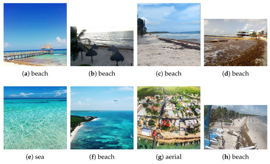
Figure 1.
Image examples from the constructed dataset.
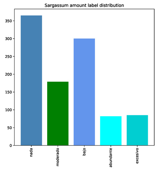
Figure 2.
Distribution of labels for characterizing the amount of Sargassum in images. The labels were defined using Spanish words. They are nada (nothing), bajo (low), moderado (mild), abundante (plenty), and excesivo (excessive).
4. Experiments and Discussion
Our target is to provide an estimation of the Sargassum amount that is present in a landscape photography of the beach. Given that the photos are taken from monocular cameras with different specifications, it is not possible to directly estimate volumes from those un-calibrated images. Therefore, we propose to use a supervised learning approach, where several known examples are given to a model and that model is trained to make predictions on unknown examples. In particular, we have modeled the problem as a classification problem, where given an image I; a model assigns it a label l from a set of predefined labels, namely:
where w and h define image’s width and height, respectively, and n is the quantization of the Sargassum level. Below, we describe the dataset that we have built, the proposed Sargassum quantization and the implementation of the model by deep convolutional neural networks.
4.1. Classification with Deep Convolutional Neural Networks
Recently, deep neural networks have proven to effectively solve several complex computer vision tasks. One advantage of such discoveries is the fact that the knowledge acquired in some context can be moved to a similar domain by using transfer learning. Transfer learning reuse the learned network weights for initializing a custom network that is intended to solve the target task. In this work, the target task is the classification of Sargassum level while the source task is the Imagenet classification [28].
There are at least two ways for using transfer learning: feature extraction and fine tuning. Feature extraction keeps the feature extraction capabilities of an already trained network by freezing the convolutional layer weights while a new classifier is attached to the feature extraction; then the new classifier is trained according to the target task. On the other hand, fine tuning replaces the classifier according to the target task and then the full network is fitted to the target task. Our hypothesis is that transfer learning can provide a good approximation of the Sargassum classification. In the next section, we present several experiments in order to validate our proposal.
4.2. Exploratory Experiments
In this experiment, we test several state-of-the art networks for the classification task using all the levels in the dataset. The tested networks are: Alexnet [25], GoogleNet [26], VGG16 [27] and RestNet18 [29]. The objective of this experiment is to characterize the effectiveness of the network architectures by validating them under three training paradigms: feature extraction (F.E.), fine tuning (F.T.), and training from ‘scratch’ (T.S.).
The parameters used are the following: epochs = 500, learning rate = 0.001 and batch size = 100. The batch size was selected as the largest amount of images that can be loaded into memory during training. The training was carried out online on a Kaggle’s virtual machine with GPU and 15 GB of memory RAM. The models were implemented in Python using the Pytorch library. Training time was 2 h on average. Overall, 80% of the dataset was used for training, while 20% was selected for validation. The best CNN weights corresponds to the epoch were the best validation accuracy was reached.
We can observe, from the results summarized in Table 1, three facts. First, the problem addressed in this work is quite different from the typical image classification problems, this is observed in the low validation accuracy (below 60%); our hypothesis is that learned features from Imagenet are not enough for this problem and that the current amount of examples is small for extracting such features. Two, fine tuning has shown the best performance during validation; this phenomenon supports our hypothesis that the features from Imagenet does not define the Sargassum because the net is learning to extract new features. Third, VGG16 has shown the best performance; we think that given the amount of available examples, the depth of VGG16 is adequate for learning features and for beating the other networks, while at the same time, it is also shallow for avoiding overfit which can be occurring with ResNet18.

Table 1.
Validation accuracy reached by each network for different training methods. Feature extraction freezes the weights in the convolutional layers. The best result for each network is remarked.
4.3. Exploitation Experiments
From the results obtained in the previous section, an exploitation grid search was performed with the architecture that presented best results, VGG16. Table 2 shows the combination of hyperparameters tested in this set of experiments. The batch size of 100 and the number of epochs of 500 were kept as orthogonal factors. The hyperparameters that were varied throughout this grid search are: learning rate and the optimizer.
Table 2.
Exploitation grid search.
The results obtained during these experiments are presented in Table 3. The adjustment in the parameters of the model showed an improvement in the classification with the combination of the optimizer Adam and the learning rate , but as can be observed, it also increases the training time of the model. It also seems that the learning rate of , regardless of the optimizer used, causes an increase in training time. Training time in all experiments ranged from approximately 2 h to 2:30 h. When the learning rate of was used in combination with the Adam optimizer, the classification accuracy drop to 36% and for 4 of the 5 classes, it was not possible to classify any image correctly, so the rest of the metrics could not be calculated.
Table 3.
Table of results obtained by the exploitation grid search. Time is displayed in minutes (min) plus seconds (s).
Figure 3 shows the confusion matrix obtained by the model using a learning rate of and Adam optimizer. the results can be better interpreted by looking at the normalized confusion matrix. It can be observed that the best performance of the model was for the excessive class, where 82 % of the images where correctly classified. This result was not expected since the number of images in this class is low in the dataset, but it is a good indicator that the model correctly identifies the characteristics in this type of images which is relevant for the detection of Sargassum when it is really abundant. The worst behavior of the model is for the class moderate for which less than half of the images were correctly classified, this is affecting the overall performance of the model since the metrics reported is the average performance over all classes.
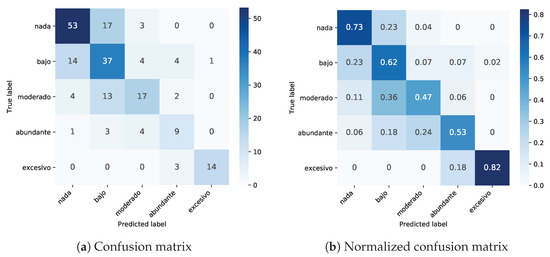
Figure 3.
Single and normalized confusion matrices for the classification of Sargassum. Translated labels are: nada (nothing), bajo (low), moderado (fair), abundante (plenty), and excesivo (excessive).
4.4. Predictions Analysis
In this section, we make a deeper analysis on the predictions provided by the model with the highest validation accuracy observed (VGG16 trained with fine tuning). From Figure 3, we can observe that predictions are near to the true label. This phenomenon is better observed in the normalized matrix (Figure 3b), where the majority of predictions are in the diagonal (true positives) and the remaining ones are distributed among the contiguous classes. This reflects the fact that there is no a hard rule for this classification, but it is based on manual labeling which is prone to the point of view of the human labeler. See Figure 4 for prediction examples. In conclusion, the predictions provided by tested models can be useful as a good approximation of the Sargassum amount.
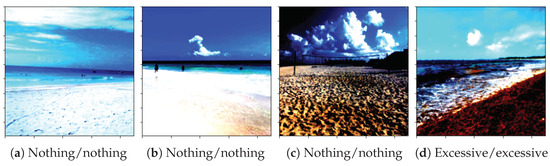
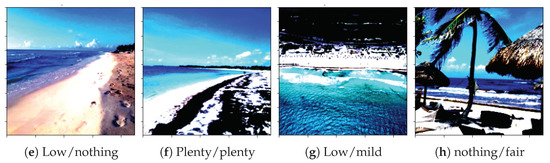
Figure 4.
Examples of Sargassum level classification using the selected convolutional neural network. Displayed images are already pre-processed: normalization and resize. The label for each example indicates: ‘predicted label/true label’.
5. Conclusions
A study for Sargassum level classification in public photographs has been presented. Several networks have been tested using different training strategies. The best results were obtained by the VGG16 model trained under fine-tuning. The best results show an accuracy of 64%. When analyzing the performance of the model with respect to each class, it was unexpected that the best behavior occurred in the excessive class, since it is one of the minority classes in the dataset, with 82% correctly classified images. This may be an indication that the model correctly extracts the features in this particular type of images. Class imbalance is another factor that may be affecting the performance of all models, so it is necessary to obtain more images of minority classes or apply class balancing methods to verify this assumption. We also hypothesize that the limited accuracy achieved by the models is bias because the levels of Sargassum in each image were assigned using human criteria. In consequence, a discrepancy between labels can be found. A stricter way for label assignment could increase the performance of the models. We hope that our system can offer a tool for Sargassum monitoring. So that, scientists, ecologists, and authorities can have a better understanding of the phenomenon. As a result, cleaning efforts and studies can be directed to critical areas. Our next research direction is to segment the Sargassum from the images and to include image geo-localization.
Author Contributions
Conceptualization and Investigation, J.I.V.; Investigation, J.I.V. and A.G.-F.; Data Curation and Software, E.V.-M.; Writing—original draft, A.V.U.-A. and H.T. All authors have read and agreed to the published version of the manuscript.
Funding
CONACYT Cátedras Project: 1507.
Institutional Review Board Statement
Not applicable.
Informed Consent Statement
Not applicable.
Data Availability Statement
All gathered data are open access and available via Kaggle: https://www.kaggle.com/datasets/irvingvasquez/publicsargazods, (accessed on 15 September 2022). The dataset will be continuously updated as new data are obtained.
Acknowledgments
The authors thank to the following people who have recollected images from public forums: Miguel Sánchez, Alberto Flores, and Cesar Pérez. The authors would like to thank the Instituto Politécnico Nacional (Secretaría Académica, Comisión de Operación y Fomento de Actividades Académicas, Secretaría de Investigación y Posgrado, Centro de Innovación y Desarrollo Tecnológico en Cómputo), Consejo Nacional de Ciencia y Tecnología, and Sistema Nacional de Investigadores for their support in developing this work.
Conflicts of Interest
The authors declare no conflict of interest.
References
- Aguirre Muñoz, A. El sargazo en el caribe mexicano: De la negación y el voluntarismo a la realidad. 2019. Available online: https://www.conacyt.gob.mx/sargazo/images/pdfs/El_Sargazo_en_el_Caribe_Mexicanopdf.pdf (accessed on 12 March 2021).
- Chávez, V.; Uribe-Martínez, A.; Cuevas, E.; Rodríguez-Martínez, R.E.; van Tussenbroek, B.I.; Francisco, V.; Estévez, M.; Celis, L.B.; Monroy-Velázquez, L.V.; Leal-Bautista, R.; et al. Massive Influx of Pelagic Sargassum spp. on the Coasts of the Mexican Caribbean 2014–2020: Challenges and Opportunities. Water 2020, 12, 2908. [Google Scholar] [CrossRef]
- Maurer, A.S.; Gross, K.; Stapleton, S.P. Beached Sargassum alters sand thermal environments: Implications for incubating sea turtle eggs. J. Exp. Mar. Biol. Ecol. 2022, 546, 151650. [Google Scholar] [CrossRef]
- Tonon, T.; Machado, C.B.; Webber, M.; Webber, D.; Smith, J.; Pilsbury, A.; Cicéron, F.; Herrera-Rodriguez, L.; Jimenez, E.M.; Suarez, J.V.; et al. Biochemical and Elemental Composition of Pelagic Sargassum Biomass Harvested across the Caribbean. Phycology 2022, 2, 204–215. [Google Scholar] [CrossRef]
- Arellano-Verdejo, J.; Lazcano-Hernandez, H.E.; Cabanillas-Terán, N. ERISNet: Deep neural network for sargassum detection along the coastline of the mexican caribbean. PeerJ 2019, 2019, e6842. [Google Scholar] [CrossRef] [PubMed]
- Balado, J.; Olabarria, C.; Martínez-Sánchez, J.; Rodríguez-Pérez, J.R.; Pedro, A. Semantic segmentation of major macroalgae in coastal environments using high-resolution ground imagery and deep learning. Int. J. Remote Sens. 2021, 42, 1785–1800. [Google Scholar] [CrossRef]
- Cuevas, E.; Uribe-Martínez, A.; de los Ángeles Liceaga-Correa, M. A satellite remote-sensing multi-index approach to discriminate pelagic Sargassum in the waters of the Yucatan Peninsula, Mexico. Int. J. Remote Sens. 2018, 39, 3608–3627. [Google Scholar] [CrossRef]
- Maréchal, J.P.; Hellio, C.; Hu, C. A simple, fast, and reliable method to predict Sargassum washing ashore in the Lesser Antilles. Remote Sens. Appl. Soc. Environ. 2017, 5, 54–63. [Google Scholar] [CrossRef]
- Sun, D.; Chen, Y.; Wang, S.; Zhang, H.; Qiu, Z.; Mao, Z.; He, Y. Using Landsat 8 OLI data to differentiate Sargassum and Ulva prolifera blooms in the South Yellow Sea. Int. J. Appl. Earth Observ. Geoinform. 2021, 98, 102302. [Google Scholar] [CrossRef]
- Wang, M.; Hu, C. Predicting Sargassum blooms in the Caribbean Sea from MODIS observations. Geophys. Res. Lett. 2017, 44, 3265–3273. [Google Scholar] [CrossRef]
- Shin, J.; Lee, J.S.; Jang, L.H.; Lim, J.; Khim, B.K.; Jo, Y.H. Sargassum Detection Using Machine Learning Models: A Case Study with the First 6 Months of GOCI-II Imagery. Remote Sens. 2021, 13, 4844. [Google Scholar] [CrossRef]
- Wang, M.; Hu, C. Satellite remote sensing of pelagic Sargassum macroalgae: The power of high resolution and deep learning. Remote Sens. Environ. 2021, 264, 112631. [Google Scholar] [CrossRef]
- Agency, T.E.S. Sentinel-2 Resolution and Swath. 2015. Available online: https://sentinels.copernicus.eu/∼/resolution-and-swath (accessed on 28 April 2021).
- Arellano-Verdejo, J.; Lazcano-Hernandez, H.E. Crowdsourcing for Sargassum Monitoring Along the Beaches in Quintana Roo. In GIS LATAM; Mata-Rivera, M.F., Zagal-Flores, R., Arellano Verdejo, J., Lazcano Hernandez, H.E., Eds.; Springer International Publishing: New York, NY, USA, 2020; pp. 49–62. [Google Scholar]
- Valentini, N.; Balouin, Y. Assessment of a Smartphone-Based Camera System for Coastal Image Segmentation and Sargassum monitoring. J. Mar. Sci. Eng. 2020, 8, 23. [Google Scholar] [CrossRef]
- Kim, J.; Kang, Y. Automatic Classification of Photos by Tourist Attractions Using Deep Learning Model and Image Feature Vector Clustering. ISPRS Int. J. Geo-Inform. 2022, 11, 245. [Google Scholar] [CrossRef]
- Alvarez-Carranza, G.; Lazcano-Hernandez, H.E. Methodology to Create Geospatial MODIS Dataset. In Communications in Computer and Information Science; Springer: Berlin, Germany, 2019; Volume 1053, pp. 25–33. [Google Scholar] [CrossRef]
- Chen, Y.; Wan, J.; Zhang, J.; Zhao, J.; Ye, F.; Wang, Z.; Liu, S. Automatic Extraction Method of Sargassum Based on Spectral-Texture Features of Remote Sensing Images. In International Geoscience and Remote Sensing Symposium (IGARSS); Institute of Electrical and Electronics Engineers: Yokohama, Japan, 2019; pp. 3705–3707. [Google Scholar]
- Sutton, M.; Stum, J.; Hajduch, G.; Dufau, C.; Marechal, J.P.; Lucas, M. Monitoring a new type of pollution in the Atlantic Ocean: The sargassum algae. In Proceedings of the OCEANS 2019—Marseille, Institute of Electrical and Electronics Engineers (IEEE), Marseille, France, 17–20 June 2019; pp. 1–4. [Google Scholar] [CrossRef]
- Wang, M.; Hu, C. Automatic Extraction of Sargassum Features From Sentinel-2 MSI Images. IEEE Trans. Geosci. Remote Sens. 2020, 59, 2579–2597. [Google Scholar] [CrossRef]
- Gao, B.C.; Li, R.R. FVI—A Floating Vegetation Index Formed with Three Near-IR Channels in the 1.0–1.24 μm Spectral Range for the Detection of Vegetation Floating over Water Surfaces. Remote Sens. 2018, 10, 1421. [Google Scholar] [CrossRef]
- Kumar, A.; Walia, G.S.; Sharma, K. Recent trends in multicue based visual tracking: A review. Expert Syst. Appl. 2020, 162, 113711. [Google Scholar] [CrossRef]
- Christin, S.; Hervet, E.; Lecomte, N. Applications for Deep Learning in Ecology. Methods Ecol. Evol. 2019, 10, 1632–1644. [Google Scholar] [CrossRef]
- LeCun, Y.; Bengio, Y.; Hinton, G. Deep learning. Nature 2015, 521, 436–444. [Google Scholar] [CrossRef] [PubMed]
- Krizhevsky, A.; Sutskever, I.; Hinton, G.E. ImageNet Classification with Deep Convolutional Neural Networks. In Proceedings of the 26th Annual Conference on Neural Information Processing Systems 2012, Lake Tahoe, NV, USA, 3–8 December 2012; pp. 1097–1105. [Google Scholar]
- Szegedy, C.; Liu, W.; Jia, Y.; Sermanet, P.; Reed, S.; Anguelov, D.; Erhan, D.; Vanhoucke, V.; Rabinovich, A. Going Deeper with Convolutions. In Proceedings of the IEEE Conference on Computer Vision and Pattern Recognition (CVPR 2015), Boston, MA, USA, 7–12 June 2015; pp. 1–9. [Google Scholar]
- Simonyan, K.; Zisserman, A. Very Deep Convolutional Networks for Large-Scale Image Recognition. In Proceedings of the 3rd International Conference on Learning Representations, ICLR 2015, San Diego, CA, USA, 7–9 May 2015; pp. 1–14. [Google Scholar]
- Russakovsky, O.; Deng, J.; Su, H.; Krause, J.; Satheesh, S.; Ma, S.; Huang, Z.; Karpathy, A.; Khosla, A.; Bernstein, M.; et al. ImageNet Large Scale Visual Recognition Challenge. Int. J. Comput. Vis. (IJCV) 2015, 115, 211–252. [Google Scholar] [CrossRef]
- He, K.; Zhang, X.; Ren, S.; Sun, J. Deep Residual Learning for Image Recognition. In Proceedings of the 2016 IEEE Conference on Computer Vision and Pattern Recognition (CVPR 2016), Las Vegas, NV, USA, 27–30 June 2016; pp. 770–778. [Google Scholar] [CrossRef]
- Vasquez, J.I. Sargazo Dataset. 2021. Available online: https://www.kaggle.com/datasets/irvingvasquez/publicsargazods (accessed on 15 September 2022).


Publisher’s Note: MDPI stays neutral with regard to jurisdictional claims in published maps and institutional affiliations. |
© 2022 by the authors. Licensee MDPI, Basel, Switzerland. This article is an open access article distributed under the terms and conditions of the Creative Commons Attribution (CC BY) license (https://creativecommons.org/licenses/by/4.0/).