Abstract
Four-dimensional seismic analysis is an effective reservoir surveillance tool to track the changes of fluid and pressure phases in the oil and gas reservoirs over time of the baseline and monitoring seismic acquisition. In practice, the 4D seismic signal associated with such changes may be negligible, especially in heterogeneous carbonate reservoirs. Therefore, 4D seismic analysis is a model for integrating various disciplines in the oil and gas industry, such as seismic, petrophysics, reservoir engineering, and production engineering. In this study, we started the 4D seismic workflow with a 1D well-based 4D feasibility study to detect the likelihood of 4D signals before performing 4D seismic co-processing of the baseline and monitoring surveys starting from the seismic field data of both datasets. As part of a full 4D seismic co-processing of the baseline and monitor surveys, 4D seismic metric attributes were analyzed over the survey area to measure the improvement in seismic acquisition repeatability for the scarce 1994 baseline seismic and the 2014 monitor seismic survey. For the monitor survey, a 4D time-trace shift was performed using the baseline survey as a reference to measure the time shifts between the baseline and monitor surveys at 20-year intervals. The 4DFour-dimensional dynamic trace warping was followed by a 4D seismic inversion to compare the 4D difference in the seismic inverted data with the difference in seismic amplitude. The seismic inversion helped overcome noise, multiple contaminations, and differences in dynamic amplitude range between the baseline and monitor seismic surveys. We then examined the relationship between well logs and seismic volumes by predicting a volume of log properties at the well locations of the seismic volume. In this method, we computed a possibly nonlinear operator that can predict well logs based on the properties of adjacent seismic data. We then tested a Deep Feed Forward Neural Network (DFNN) on six wells to adequately train and validate the machine learning approach using the baseline and monitoring seismic inverted data. The objective of trying such a deep machine learning approach was to predict the density and porosity of both the baseline and the monitoring seismic data to validate the accuracy of the 4D seismic inversion and evaluate the changes in reservoir properties over a time-lapse of 20 years of production from 1994 to 2014. Finally, we matched the 4D seismic signal with changes in reservoir production properties, investigating the mechanism underlying the observed 4D signal. It was found that the detectability of 4D signals is primarily related to changes in fluid saturation and pressure changes in the reservoir, which increased from 1994 to 2014. This innovative closed-loop research proved that the low repeatability of seismic acquisition can be compensated by optimal 4D seismic co-processing with a complete integration workflow to assess the reliability of the 4D seismic observed signal.
1. Introduction
Although seismic monitoring has been conducted on numerous projects, most success has been on clastic offshore reservoirs where seismic time-lapse conditions are most favorable. In the area of study, in December 2013, a 4D seismic monitor survey was conducted in the study area with an OBC 3D seismic survey over this selected field and completed in November 2014, while the baseline survey was acquired as a 3D OBC in 1994. OBC acquisition was found to have a very high level of random noise in both phases. OBC acquisition with only one sensor is very sensitive to noise (seafloor currents, Schulte waves, ship noise, etc.). We recommend OBN (Ocean Bottom Node) and "nodes on a rope", especially because of the shallow water in this offshore field in Abu Dhabi, UAE. With OBN; because the shape of such a sensor (a disc) should be less sensitive to seabed currents and industrial noise (and the Schulte wave should be the same). Also, it is very useful to record the seawater velocity profile and sea water depth during seismic acquisition to have a good possibility for anti-multiple seismic processing. For this reason, ADNOC has conducted the world’s largest continuous 3D onshore and offshore seismic surveys in Abu Dhabi with very high specifications for seismic acquisition parameters. For offshore seismic, a 3D OBN seismic acquisition type was acquired, to provide 2400 seismic coverage with 6 km inline and crossline offsets. The acquisition began in late 2018 and is expected to be completed by the end of 2022, with final images delivered two years later. This is an extremely tight schedule considering that nearly 90,000 km2 need to be covered [1].
Despite extensive acquisition efforts, time-lapse processing is an essential component to obtain highly repeatable data [2]. Although hydrocarbon production from carbonates is a significant part of the world’s energy supply, 4D seismic data have been more successful in monitoring hydrocarbon production from clastic reservoirs [3,4]. Four-dimensional seismic data are widely used in the oil and gas industry to image fluid movement and contacts, monitor flow paths and barriers, locate bypassed oil, place new wells, identify sealing faults, and map pressure compartmentalization and thermal effects [5].
An accurate description of the reservoir is useful to properly manage and optimize oil recovery. When moving from the core to seismic scale, all relevant information must be combined to reduce uncertainties, optimize final flow behavior, and determine fluid distribution in the reservoir [6]. The oil of the reservoir at the area of study has an average gravity of 37 API, while the gas gravity is 0.816. On the other hand, the GOR (gas-oil ratio) is 2300 Scf/bbl at a pressure of 4400 PSI and a temperature of 80 degrees Celsius. Initial production provided enough data on the reservoir so that reservoir behavior could be well studied and simulated. Water injection supported reservoir pressures, and injectivity tests were conducted to ensure the feasibility of injecting water into the formation [7]. Four-dimensional seismic data can provide valuable information on production scenarios related to saturations and pressure variations, therefore, 4D seismic-derived attributes (such as amplitude and impedance changes) are highly recommended to provide accurate seismic interpretation in conjunction with a 4D seismic study [8]. Moreover, combinations of pressure and fluid saturation variations dominate the seismic response and influence its direct interpretations [9].
Carbonate reservoirs are generally heterogeneous and have high rock-frame stiffness, which could complicate the use of 4D seismic data to monitor fluid changes in carbonate rocks. The main objective of this study was to evaluate the detectability of a 4D signal between two non-repeatable seismic surveys and to determine how best to process the seismic data and link it to non-seismic relevant information to measure the credibility of the 4D seismic signal [10,11]). To compensate for the poor repeatability of the acquisition geometry between the baseline and monitor surveys (different coordinates of the source and receiver, different azimuths, and the number of obstructions), 4D seismic co-processing with field tapes for both the baseline and monitor surveys was used in this study. Deliberate full seismic 4D co-processing starting from the seismic field records is more accurate and robust, and thus far more repeatable, than partial seismic 4D co-processing with Kirchhoff Pre-stack depth migration (KPSDM) or Least Square Pre-stack depth migration (LSM) [12].
Differences in the subsurface cause changes in amplitudes and velocities, resulting in the misalignment of the seismic reflectors. Measuring the misalignment and aligning these surfaces to obtain a reliable differential cube is one of the most important disciplines in 4D seismic processing [13]. One of the most important calibration steps in the time-lapse seismic workflow is the calculation of the optimal dynamic time and space shifts required to calibrate multiple monitor surveys with a baseline survey. Dynamic Time Warping is useful for lining up seismic images from different time-lapse periods, especially for determining the time-variant time shifts. The accuracy of Dynamic Time Warping (DTW) in estimating similarity is being investigated for template matching and clustering of seismic traces [14].
The conversion of seismic reflection data into physical properties of the subsurface, such as elastic parameters, is called seismic inversion [15]. These properties can be correlated with porosity, lithology, fluid saturation, and geomechanical properties [16]. Choosing the most accurate and robust analysis domain is particularly important in 4D time-lapse studies [17], so seismic inversion in 4D can be more effective than regular seismic wiggle-trace work in this regard. Time-lapse (4D) seismic inversion aims can be used to predict changes in elastic rock properties, such as acoustic impedance, from measured seismic amplitude variations due to hydrocarbon production. The goal of seismic inversion is to determine a reservoir model that minimizes the errors between predicted seismic amplitudes and observed seismic amplitudes [18].
A low-frequency anomaly is usually associated with fluid in the reservoir, while a high-frequency anomaly is associated with gas or clay content of the reservoir [19]. The main challenges in 4D seismic analysis are improved 4D vertical resolution (ideally 1–10 m), improved repeatability that enables an application to carbonate reservoirs, and innovative ways to combine 4D seismic data with other reservoir measurements and simulation methods [20]. In this study, we used a hybrid theory and data model to evaluate the results of 4D seismic inversion and predict changes in reservoir rock properties over 20 years, such as density and porosity, from baseline and monitor surveys.
We used a software package from Hampson-Russell (Emerge) that analyzes well logs and seismic data by establishing a relationship between logs and seismic data at well locations. Deep learning was tested against a single attribute list of individual features from a nonlinear regression curve method. The network is used in geophysics to quantitatively predict rock properties from seismic data [21]. In supervised learning, we gave the neural network a set of inputs and outputs for a given problem and let it determine the relationship between those inputs and outputs. The drawback of supervised learning is that enough inputs and outputs are needed to adequately train the network [22].
Matching the observed 4D signal with reservoir performance over the entire production span of the baseline survey in 1994, and the monitor seismic survey in 2014, is evidence that 4D seismic co-processing can fill up the gap left by poor repeatability of seismic acquisition. The mechanism of 4D signal generation was explained by the increase in fluid saturation for oil and water with pressure rise over the 20 years of the 4D time-lapse.
2. Materials and Methods
We began this innovative, integrative study by first conducting a 4D feasibility study to complement the core research and identify best practices for future 4D seismic work in the seismic industry. The feasibility study included petro-elastic modeling and 1D well-based time-lapse 4D modeling. The objective of conducting this part of the research was to evaluate the detection of changes in seismic response probability caused by field production at the reservoir level and ultimately to support the actual 4D interpretation of seismic results. Petro-elastic model (PEM) and 1D time-lapse modeling of the research area support the 4D signal from well production and injection data. A fluid substitution tool performed substitution of fluids from an initial reservoir state to a new state and examined the effects of this fluid substitution on the elastic properties of the reservoir [23].
1D Well-Based Time-Lapse Feasibility Study
The petro-elastic model was built (Figure 1a) with the following main steps:
- Mix mineral properties.
- Add pores using effective media theories.
- Calculate fluid properties.
- Perform fluid substitution.
Fluids are introduced into pore space using the equations of Gassmann [24], using the results of the last three steps. Gassmann’s relations are often used to predict the modulus of saturated rock from the modulus of dry rock, and vice versa. The most common in situ problem is to predict the changes that occur when one fluid is replaced by another that has both mineral and dry bulk moduli and fluid properties. Here, we used the normal Gassmann equation to introduce the effective fluid into the empty pores included in the matrix. The Gassmann substitution of fluid was used to calculate the effective saturated properties (Figure 1b).
The research activities were divided into three phases. The first phase involved a well-based (1D) time-lapse model using a production well with gassy carbonate at the crest of the structure and an injection well at the flank of the structure. The 4D modeling covered a range of possible production scenarios expected in the field, including changes in water saturation due to water injection and changes in gas saturation due to pressure changes. Feasibility of the 4D approached was investigated by running an appropriate petro-elastic model and a 1D time-lapse with production and injection data to investigate the detectability of 4D signals and determine how these could relate the modeling to actual 4D seismic.

Figure 1.
(a) Physics model for carbonate rocks after [25], and (b) fluid substitution saturated Properties after [24].
Petrophysical analysis confirmed that two minerals should be used for the reservoir to model the matrix. The elastic properties used for these minerals were standard values, but they were also derived from data analysis during petrophysical interpretation, as was their volume fraction. In the area of the reservoir under study, we determined the average porosity by experimenting with statistics from several wells within the main reservoir zone. The overall average porosity was about 15PU, with the K-frame being relatively loose because the reservoir zone is a mixture of dolomite and calcite. These elastic values are listed in Table 1. In addition, this study used the Voigt-Reuss-Hill model [26], to mix these minerals:

Table 1.
Reservoir elastic properties.
The reservoir fluids and the dry rock elastic properties, computed from the PEM, were combined in the Gassmann’s (1951), equation to calculate the saturated elastic moduli at different reservoir conditions:
- −
- In-situ (pre-production).
- −
- Water displacing gas to different saturations: 10, 50 and 85%.
- −
- CO2 displacing gas to different saturations: 10, 50 and 85%.
The expected 4D field impacts were evaluated by a well-based (1D) fluid substitution feasibility study. This 1D model tested three possible production scenarios that could be expected in the field. Changes in water saturation due to water injection and three scenarios of gas saturation in this gas-bearing reservoir due to pressure changes were modeled. The predicted 4D response was evaluated using synthetic seismic angles between zero and 45 degrees obtained from P-wave, S-wave, and density logs from a production well and an injection well. A 30 Hz Ricker wavelet was fitted to generate the synthetic gathers corresponding to the dominant frequency of the reservoir-level seismic data.
In the gas-producing well, density was reduced at 10% water flooding compared to 50% and 85% water flooding, while the change in VP/VS was very small compared to the change in density. Moreover, the synthetic gather angles were generated with different percentages of water flooding (Figure 2a), showing a 4D difference between the baseline (in-situ) and the different production scenarios that were much stronger at 50 to 85% saturation (Figure 2b). CO2 sweeping was not optimal in the gas-producing well because it is a gas-bearing reservoir. Therefore, we decided to omit this scenario.
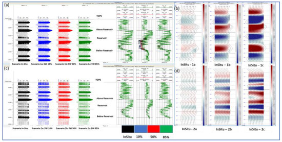
Figure 2.
(a) Gas production well with different water saturation scenarios—angle of synthetic gathers with corresponding log tracks (b) Gas production well: angle stack of differences between in-situ and different SW (c) Water injection well with different water saturation scenarios—angle of synthetic gathers with corresponding log tracks, 4D difference of three water saturation scenarios and (d) water injection well: angle stack of differences between in-situ and different SW.
However, in the water injection well, successfully modeled synthetic angular logging of water flooding was measured with the corresponding log traces (Figure 2c). The 4D effects are evident from the difference between the angle of in-situ and the different water saturation scenarios of the water injection well (Figure 2d). The 4D difference was stronger at 85% flowing water than at 50%, while there was little difference at 10%. There was a sharp increase in density and the ratio VP/VS, which reflects an increase in acoustic impedance of more than 10% at the reservoir level.
The 4D effects were visible in the differences between the in-situ angle gather and the angle gather of the different scenarios of CO2 gas displacement of the water in the injection well. The 4D difference for gas injection was generally stronger than for the water saturation scenarios. While 85% water saturation data was close to that of 50%, it was slightly stronger than 10% for CO2 gas displacement (Figure 3b).
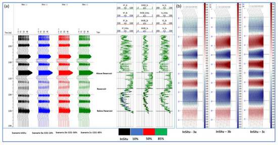
Figure 3.
(a) Water injection well with different CO2 saturation scenarios: angle synthetic gathers with corresponding log tracks (b) Water injection well: angle stack of differences between in-situ and different CO2 saturations.
Comparison of P impedance (IP) and shear impedance (IS) for different production scenarios for gas-producing wells or for wells with water injection showed that a water sweep with different scenarios for both wells can change P impedance by about 4% and shear impedance by 3%, while a CO2 sweep can change P impedance by about 8% and shear impedance by 2% (Figure 4a,b). On the other hand, in the water sweep region, the P impedance was expected to change by about 4% and the VP/VS ratio by 3%, and the CO2 sweep led to a change in the P impedance by about 8% and the VP/VS ratio by 8% (Figure 4c,d). Thus, the expected changes were greater than 4%, which is the value usually considered detectable by experience and the literature [27]. The petro-elastic model and 1D time-lapse pave the way to link the production data with the current seismic data and measure the similarity between them. The petro-elastic model and the 1D time-lapse model led to the following conclusions:
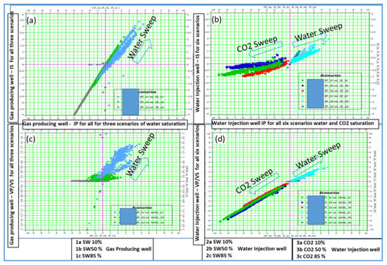
Figure 4.
(a) Cross-plot of P impedance versus IS (shear impedance) for three water saturation scenarios of the gas production well; (b) cross-plot of P impedance versus IS (shear impedance) for six water saturation scenarios of CO2 saturation of the water injection well; (c) cross-plot of P impedance versus VP/VS ratio for three water saturation scenarios of the gas production well, and (d) cross-plot of P impedance versus VP/VS for six water saturation and CO2 saturation scenarios of the water injection well.
For water injection wells:
- Matching with the in-situ situation showed the validity of the rock physics model used, i.e., the Gassmann fluid substitution performed, and the accuracy of the measured logs.
- The water-sweep scenarios showed minimal changes in the logs, indicating that water flooding in an oil reservoir is relatively difficult to quantify on a time-lapse seismic image.
- For the same oil reservoir, on the other hand, CO2 flooding showed stronger changes, especially in P-wave velocity and thus impedance, making CO2 sweep scenarios more observable on time-lapse seismic.
- It is quite clear that CO2 showed pronounced signatures in the form of acoustic impedance changes.
For the producing well:
- The matching with the in-situ situation showed some discrepancy between the measured log and the log produced by the rock physics, especially in the very porous sections of the reservoir.
- The water sweep scenarios showed some degree of change in the logs, suggesting that a water flood may be observable in the gas reservoir on a time-lapse seismic image.
3. Results & Discussion
3.1. 4D Seismic Co-Processing
For such non-repeatable 4D seismic acquisition surveys of the study area, 4D seismic co-processing was started with the field-recorded seismic data from both the baseline and monitor surveys. Pre-processing, including noise reduction, static computation, and de-multiple with predictive 3D deconvolution, allowed successful adjustment of overburden phase and amplitude, and the reservoir level remained intact. Four-dimensional binning was performed using the adjacent offset classes from the 1994 baseline survey to select retained traces with a Distance Source, Distance Receiver (DSDR) value of less than 200 m for offset classes 1 through 16, and less than 300 m for offset classes 17 through 62, followed by 5D Fourier bin regularization including noise attenuation. To close the repeatability gap, it was decided to test the pre-stack least squares depth migration algorithm (LSM) against the Kirchhoff pre-stack depth migration algorithm (KPSDM).
The pre-stack seismic depth imaging workflow began with Kirchhoff (KPSDM) for the baseline and monitor surveys. Then, the original Kirchhoff OVTs were de-migrated for depth imaging and least square migration (LSM). Kirchhoff KPSDM was applied to both baseline and monitor surveys. To this end, both datasets were recursively migrated after preprocessing and de-migrated at each iteration using Hessian filter calculations in the Curvelet domain to create a reflectivity model for each vintage. The baseline and monitor surveys were then finally de-migrated to baseline coordinates. Before the final reflectivity models were created, three iterations of migration and de-migration were performed. The seismic processing step of least-square migration used input data without 3D regularization for both the baseline and monitor surveys. Therefore, the LSM results were clean data compared to the Kirchhoff PSDM, which used inputs after 3D regularization. The LSM seismic difference had a much lower difference level compared to the Kirchhoff PSDM seismic difference, indicating that the Kirchhoff LSM pre-stack depth migration algorithm appeared to mitigate some of the non-repeatable seismic noise. The seismic difference between the baseline and the monitor was clearly visible on the crest of the structure compared to the adjacent seismic traces (Figure 5c).
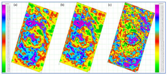
Figure 5.
Horizon slice on a window between the upper and lower parts of the reservoir of the final migrated seismic stack volume: (a) baseline seismic volume; (b) monitor seismic volume, and (c) the seismic difference between baseline and monitor surveys. Block polygon that includes the high amplitude difference at the crest of the reservoir.
Diagnostic 4D QC attributes were extracted at each stage of 4D seismic co-processing, e.g., NRMS were examined to ensure that vintages become increasingly comparable. Deterministic pre-stack corrections were strongly recommended rather than relying solely on post-stack matching. This rigorous approach ensured that 4D noise was more accurately captured and the 4D reservoir signature was preserved [28]. The 4D signal can be measured by the Normalized Root Mean Square (NRMS) attribute, which is defined as the difference between two normalized data sets RMS. NRMS is routinely used as a quality control measure for time-lapse data [29]. The sensitivity of the NRMS value to the repeatability of the recording geometry has been described in several publications [30,31].
We conclude that the final NRMS value was regularly discarded to quantify the quality of the 4D signal. Predictability was used to measure the repeatability or coherence between two data sets. Repeatability is regularly evaluated using the normalized RMS difference and predictability, which is usually the normalized cross-power or coherence of the difference between the baseline and monitor surveys. For a seismic acquisition with poor repeatability, the predictability is between 0 and 65%, while perfect predictability should be above 85%. The difference between predictability and NRMS showed that the cross-correlation methods were not very sensitive to subtle 4D effects (Rocco Detomo, 2013). We extracted the above NRMS attributes of KPSDM versus seismic LSM volumes for 4D seismic. The NRMS means of the seismic volume of KPSDM was almost 15% (Figure 6a) and the NRMS mean for the final migrated LSM stack reached less than 12% (Figure 6b). This shows that the full 4D seismic co-processing with LSM is more repeatable than KPSDM.
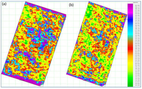
Figure 6.
Horizon slice of reservoir level: (a) NRMS of KPSDM seismic volume, and (b) NRMS of LSM seismic volume.
3.2. Seismic Inversion and Supervising Machine Learning Neural Network
After completion of 4D seismic co-processing, 4D seismic interpretation was performed to investigate the 4D time shift between the baseline and the monitor’s final migrated stack volume. The time shift is as important as the seismic 4D amplitude differences. A dynamic time shift was calculated for the final migrated seismic volume of the monitor with a time window of 1000 to 2000 ms and a threshold of ±8 ms, using the baseline survey as a reference. Due to the 4D warping time shift, the baseline and monitor seismic volumes converged in time and amplitude compared to the volume without 4D warping. We calculated the velocity variation (DV) by scripting the 4D warping time-shift volume between the baseline seismic volumes and the final migrated seismic volumes. We calculated the low-frequency model of the warped seismic monitor volume using the DV changes in the volume as input with the low-frequency P-impedance model of the baseline survey. The baseline seismic volume and the warped monitor seismic volume were combined into a super group, as was the low-frequency model of the baseline and monitor surveys. A deterministic model-based 4D seismic inversion was created using well and seismic information for both the baseline and monitor surveys. The P-impedance, which is the result of the seismic inversion, was matched with the impedance calculated from the well logs to predict the 4D differences in rock properties such as density and porosity.
We then used the Hampson-Russell (Emerge) software program, a procedure designed to merge well logs and seismic data. The general objective was to predict a property of the well log based on attributes of the seismic data. This property can be any measured log type, such as velocity or porosity, or even a derived lithologic attribute, such as shale volume. The seismic attributes can be calculated internally or provided as external attributes. The analysis was performed in several steps:
- (1)
- Examine the log and seismic data at well locations to determine which set of attributes is appropriate.
- (2)
- Derive a relationship using multi-linear regression or Neural Networks.
- (3)
- Apply the derived relationship to a 3D SEG-Y volume to create a volume of the desired log property.
We tested six wells and thirteen wells with the baseline and monitor 4D seismic inversion volumes to train the data and investigate whether we could achieve a better match between the predicted density and the original density of the well logs using two approaches. The first approach was a single attribute regression curve to calculate the correlation coefficients for all attributes and rank their values by testing the nonlinear transformation applied to the target logs of wells penetrating the reservoir. The calculated average error is the root-mean-square difference between the target log values and the predicted values calculated over the analysis window for all selected wells. Note that applying a regression curve to the 1/(inversion) produces a result that reflects the general trend of the target logs but does not adequately predict the subtle features. This is because the inversion was blocked with a relatively coarse block size. The second task was to test the deep feed forward neural network (DFNN). In this deep machine learning approach, we used three hidden layers with a total of 50 training and validation iterations using six wells. For six wells, the agreement between the predicted density and the original density was better than for the thirteen wells, and the DFNN approach had the best match between predicted density (black curve) and the original density (red curve) (Figure 7c). It was clear that machine learning approach provided the best fitting between the predicted density and the actual density compared to the single attribute regression curve method using six wells for training and validation (Figure 7f).
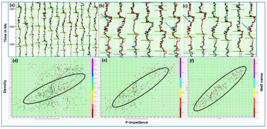
Figure 7.
Predicted density from well logs and seismic inverted volumes overlying well logs with original density. (a) 13 well log traces, (b) 6 well log traces, (c) DFNN six well log traces, (d) 13 wells, that match between predicted and actual density, (e) 6 wells that match between predicted and actual density, and (f) 6 well logs that match between predicted and actual density using machine learning with DFNN. The blue rectangle encloses the interval of reservoir logging. The target logs are colored black, while the predicted logs are red. The blue arrow indicates the similarity of the actual and predicted densities of six well logs with and without machine learning with DFNN, and the black oval highlights the fit.
We applied the DFNN operator to the seismic inversion dataset for both the baseline and monitor surveys and compared it to other paths, either 13 wells or 6 wells. DFNN provided a higher resolution result than the nonlinear transformation regression curve approach using the 6-well and 13-well tests and appeared to match the well better, especially in the reservoir interval of the target logs (Figure 8).
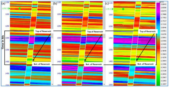
Figure 8.
A subline over the predicted seismic density volume with the actual density log of the intersected well (a) 13 wells used to train and validate the data; (b) 6 wells used to train and validate the data, and (c) 6 wells with the machine learning approach. The black rectangle encloses the reservoir interval, and the black arrow indicates the resolution differences between the different paths.
We used the six-well trained nonlinear regression approach to predict porosity using seismic volume with predicted density and compared it to DV velocity variations between baseline and monitor surveys and 4D seismic inversion of P impedance. It clearly showed that we had a negative DV with a lower P-impedance at the reservoir level, reflecting a lower density and a higher porosity of almost 14%, which is quite close to the average total porosity of 15 PU from the Petro-elastic model mentioned earlier (Figure 9). To understand the seismic response of a reservoir whose acoustic impedance (density × velocity) is lower than that of the trapped gas, it is necessary to understand that velocity and density increase as the water replaces the oil, resulting in acoustic hardening. However, in this study, it was found that gas replaces oil when velocity and density decrease. This leads to acoustic softening, which leads to an increase in seismic amplitude and a downward time shift [32].
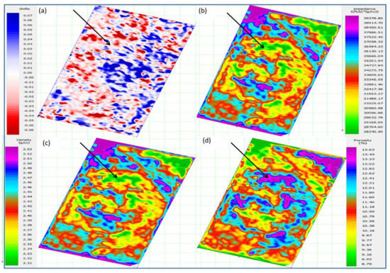
Figure 9.
Reservoir horizon slice. (a) DV velocity variation between baseline and monitor survey: (b) P impedance of seismic monitor survey: (c) monitor-predicted density, and (d) monitor-predicted porosity. The decrease in DV, impedance, and density and the increase in porosity are indicated by the black arrow.
3.3. Matching of 4D Seismic Signal with Reservoir Performance
Viewing reservoir performance in 4D time-lapse between the 1994 baseline survey and the 2014 monitor survey, we created maps of reservoir saturation properties from the dynamic reservoir simulation model to match the variation in these properties with the change in seismic response over 20 years. The simulator had embedded computational equations with several theories that could upscale the static model. It was found that water injection was about 4% in 1994 and less than 2% in 2014 (Figure 10a). Gas injection, on the other hand, was near zero Million Standard Cubic Feet (Mscf)/day in 1994, then increased to 800 K Mscf/day and decreased to 400 K Mscf/day in 2014 (Figure 10b).
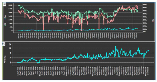
Figure 10.
Reservoir performance over time. (a) Water injection, (b) gas injection. The white arrow shows the 4D time-lapse between the base year 1994 and the monitoring year 2014, showing a decrease in water injection with a simultaneous increase in gas injection.
Oil and gas saturation increased simultaneously throughout the production period; gas saturation reached about 120,000 Mscf/day in 1994 and increased to about 450,000 Mscf/day, while oil saturation increased from about 200,000 Mscf/day in 1994 to 240,000 Mscf/day, However, in 1994, water saturation was near zero Mscf/day and then gradually increased to less than 40,000 Mscf/day (Figure 11a). In addition, the water cut was zero in 1994 and increased to 12% by 2009, then decreased to 4% by 2014 (Figure 11b).
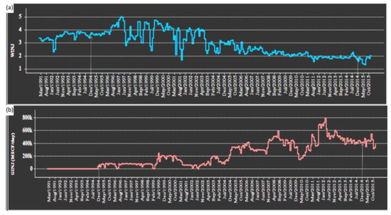
Figure 11.
Reservoir performance over time. (a) Oil, gas, and water saturation in Mscf/day and (b) water cut %.
The average map of reservoir pressure changes over time shows that the pressure was about 3600 PSI in 1994 and increased to about 3900 PSI in 2014. The average pressure difference over 20 years shows a change of less than 300 PSI to maintain reservoir pressure and production (Figure 12).
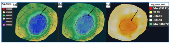
Figure 12.
Reservoir performance over time—average pressure changes. (a) 1994 baseline, (b) 2014 monitor and (c) difference of pressure between baseline and monitor. The crest of the structure is indicated by a red polygon and a black arrow indicating the maximum pressure difference.
Moreover, the maps of average oil and water saturation show that average oil saturation had almost decreased due to production, while water saturation had increased by about 30%, which can be clearly seen on the map of average difference (Figure 13c–f).
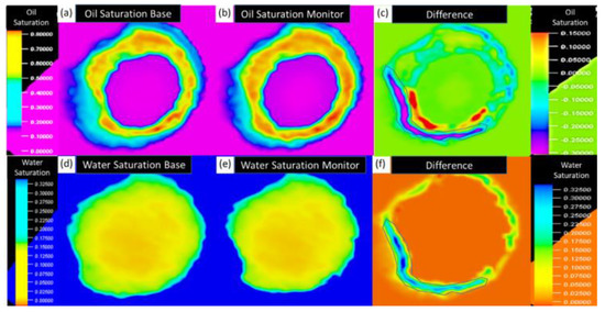
Figure 13.
Reservoir performance over time of average saturation. (a) Oil saturation baseline 1994, (b) oil saturation monitor 2014, (c) oil saturation difference, (d) water saturation baseline 1994, (e) water saturation monitor 2014, and (f) water saturation difference. The black polygon shows the significant decrease and increase in oil and water saturation, respectively.
Based on what has been shown so far in this study, we can easily relate the pressure changes to the difference in seismic amplitude of the final migrated stack of the baseline and monitor survey when trying to understand the structure of the predicted 4D signal. In the polygon of the noticeable changes, we saw in pressure saturation could be overlaid the seismic amplitude difference between the 1994 baseline and the 2020 seismic monitor survey (Figure 14). As gas takes the place of oil, velocity, and density decrease, resulting in acoustic attenuation that is reflected in an increase in seismic amplitude and a downward shift in time.
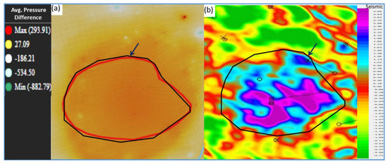
Figure 14.
(a) Changes in pressure saturation over the 20-year period, and (b) horizon slice difference between baseline and the monitor survey. The black polygon indicates the average pressure difference and the higher amplitude of the seismic difference.
4. Conclusions
This research has shown an unprecedented way to conduct a 4D analysis in a closed loop starting from a feasibility study and passing through optimum 4D seismic co-processing to 4D seismic inversion. A deep learning approach was used to show that extraction of density and porosity prediction volumes can check the success of the 4D seismic inversion outcome. Furthermore, matching the observed 4D seismic signal with e changes in fluid saturation and pressure changes of the reservoir performance checked the validity of 4D signal detectability.
The feasibility study showed that the CO2 injection scenarios allowed detection of changes in impedance and VP/VS ratio expected in 4D by more than 8%, which was demonstrable from the perspective of detectability of 4D responses. This study proved that full 4D seismic co-processing for baseline and monitor surveys from field tapes is the best approach for 4D seismic analysis. In addition, resilient pre-processing in the form of noise and multiple reductions and least square prestack depth migration is a method for mitigating the poor repeatability of seismic acquisition between baseline and monitor surveys. Given the level of detail and full integration we obtained in this seismic 4D study, we can say with confidence that repeatability of seismic acquisition will no longer be an obstacle to successful seismic 4D work in general, and in carbonate in particular.
Author Contributions
M.M. developed the workflow for re-processing and 4D analysis, Y.B. reviewed the paper and contributed to enhancement in methodology, A.A.B. reviewed and edited, and A.N. conducted formal analysis of the paper. All authors have read and agreed to the published version of the manuscript.
Funding
This research was funded by “Ministry of Higher Education Malaysia for Fundamental Research Grant Scheme with Project Code: FRGS/1/2022/STG08/USM/02/1”.
Institutional Review Board Statement
Not applicable.
Informed Consent Statement
Not applicable.
Data Availability Statement
Data sharing not applicable.
Acknowledgments
The authors would like to thank the management of ADNOC (Abu Dhabi National Oil Company) and USM (Universiti Sains Malaysia) for permission to publish this work. We would like to acknowledge “Ministry of Higher Education Malaysia for Fundamental Research Grant Scheme with Project Code: FRGS/1/2022/STG08/USM/02/1”. Finally, thanks to my colleagues Olivier Kirstetter, Ahmed Saeed Alkaabi, and Basma El Shamouty for their help and contribution, and Shraddha Chatterjee and Santan Kumar of Geosoftware Company for their help and guidance in using the Hampson Russel software.
Conflicts of Interest
The authors declare no conflict of interest.
References
- Cambois, G.; Al Mesaabi, S.; Casson, G.A.; Cowell, J.; Mahgoub, M.; Al Kobaisi, A. The World’s Largest Continuous 3D Onshore and Offshore Seismic Survey Sets Ambitious Quality and Turnaround Targets. In SEG Technical Program Expanded Abstracts; OnePetro: Richardson, TX, USA, 2019. [Google Scholar]
- Smith, R.; Hemyari, E.; Bakulin, A.; Alramadhan, A. Making seismic monitoring work in a complex desert environment—4D processing. Geophysics 2019, 38, 637–645. [Google Scholar] [CrossRef]
- Calvert, R. Insights and Methods for 4D Reservoir Monitoring and Characterization: SEG/EAGE DISC (Distinguished Instructor Lecture Course. 2005. Available online: https://library.seg.org/doi/abs/10.1190/1.9781560801696 (accessed on 23 June 2021).
- Sarkar, S.; Gouveia, W.P.; Johnston, D.H. On the inversion of time-lapse seismic data. SEG Tech. Program Expand. Abstr. 2003, 22, 1489–1492. [Google Scholar]
- Niri, M.E. 3D and 4D Seismic Data Integration in Static and Dynamic Reservoir Modeling: A Review. Pet. Sci. Technol. 2018, 8, 38–56. [Google Scholar] [CrossRef]
- Pacheco, C. Predicting Pressure and Fluid Saturation Changes Using 4D Seismic Attributes, Production Data and Simulation Model, FORCE, 30 Years of 4D Seismic on the Norwegian Continental Shelf. 2018. Available online: https://www.npd.no/globalassets/2-force/2019/bilder-og-illustrasjoner/seminars/previous-seminars/30-years-of-4d-seismic-on-the-ncs/predictingpressuresandfluidsaturations4d-2.pdf (accessed on 12 July 2021).
- Downie, W.A.; Hood, B.F. Development of the Umm Shaif Field in Abu Dhabi. In Proceedings of the Arab Petroleum Congress, Dubai, United Arab Emirates, 10–16 March 1975; Volume 130. [Google Scholar]
- Bashir, Y.; Faisal, M.A.; Biswas, A.; Babasafari, A.A.; Ali, S.H.; Imran, Q.S.; Siddiqui, N.A.; Ehsan, M. Seismic expression of Miocene carbonate platform and reservoir characterization through geophysical approach: Application in central Luconia, offshore Malaysia. J. Pet. Explor. Prod. Technol. 2021, 11, 1533–1544. [Google Scholar] [CrossRef]
- Maleki, M.; Davolio, A.; Schiozer, D.J. Qualitative time-lapse seismic interpretation of Norne Field to assess challenges of 4D seismic attributes. Geophysics 2018, 37, 754–762. [Google Scholar] [CrossRef]
- Babasafari, A.A.; Rezaei, S.; Sambo, C.; Bashir, Y.; Ghosh, D.P.; Salim, A.M.A.; Yusoff, W.I.W.; Kazemeini, S.H.; Kordi, M. Practical workflows for monitoring saturation and pressure changes from 4D seismic data: A case study of Malay Basin. J. Appl. Geophys. 2021, 195, 104472. [Google Scholar] [CrossRef]
- Babasafari, A.A.; Bashir, Y.; Ghosh, D.P.; Salim, A.M.A.; Janjuhah, H.T.; Kazemeini, S.H.; Kordi, M. A new approach to petroelastic modeling of carbonate rocks using an extended pore-space stiffness method, with application to a carbonate reservoir in Central Luconia, Sarawak, Malaysia. Geophysics 2020, 39, 592a1–592a10. [Google Scholar] [CrossRef]
- Mahgoub, M.; Bashir, Y.; Bery, A.A.; Noufal, A.W. 4D seismic co-processing pre-stack depth migration for scarce acquisition repeatability. J. Pet. Explor. Prod. Technol. 2022, 1–15. [Google Scholar] [CrossRef]
- Dramsch, J.S.; Christensen, A.N.; MacBeth, C.; Luthje, M. Deep Unsupervised 4D Seismic 3D Time-Shift Estimation with Convolutional Neural Networks. 2019. Available online: https://eartharxiv.org/repository/view/592 (accessed on 15 February 2021).
- Kumar, U.; Legendre, C.P.; Zhao, L.; Chao, B.F. Dynamic Time Warping as an Alternative to Windowed Cross Correlation in Seismological Applications. Seism. Res. Lett. 2022, 93, 1909–1921. [Google Scholar] [CrossRef]
- Tarantola, A. Inverse Problem Theory and Methods for Model Parameter Estimation; Society for Industrial and Applied Mathematics (SIAM): Philadelphia, PA, USA, 2005. [Google Scholar] [CrossRef]
- Frazer, B.; Andres Bruun, A.; Alfaro, J.K.; Roberts, R. Seismic Inversion Reading between the Lines, Oilfield Review. 2008. Available online: https://www.slb.com/-/media/files/oilfield-review/seismic-inversion (accessed on 25 December 2020).
- Souza, R.; Lumley, D.; Shragge, J. Estimation of reservoir fluid saturation from 4D seismic data: Effects of noise on seismic amplitude and impedance attributes. J. Geophys. Eng. 2017, 14, 51–68. [Google Scholar] [CrossRef][Green Version]
- Francis, A. Limitations of deterministic and advantages of stochastic seismic inversion. CSEG Recorder 2005, 30, 5–11. [Google Scholar]
- Goloshubin, G.; Silin, D. Using frequency-dependent seismic attributes in imaging of a fractured reservoir zone. In Proceedings of the 2005 SEG Annual Meeting, Houston, TX, USA, 6–11 November 2005. [Google Scholar]
- Landrø, M.; Amundsen, L. 4D Seismic—Status and Future Challenges; GEO ExPro; Energy & Geoscience Institute Salt Lake City: Salt Lake City, UT, USA, 2007. [Google Scholar]
- Downton, J. Deep Neural Networks to Predict Reservoir Properties from Seismic CGG-Geosoftware. 2018. Available online: www.cgg.com (accessed on 15 May 2022).
- Quirein, J.; Hampson, D.; Schuelke, J. Use of multi-attribute transforms to predict log properties from seismic data. In Proceedings of the EAGE Conference on Exploring the Synergies between Surface and Borehole Geoscience-Petrophysics meets Geophysics, Paris, France, 6–8 November 2000. [Google Scholar]
- Webb, B.; Rizzetto, C.; Pirera, F.; Paparozzi, E.; Milluzzo, V.; Mastellone, D.; Marchesini, M.; Colombi, N.; Buia, M.; Bertarini, M. 4D seismic opportunity: From feasibility to reservoir characterization—A case study offshore West Africa. First Break 2019, 37, 69–77. [Google Scholar] [CrossRef]
- Gassmann, F. Elastic Waves through a Packing of Spheres. Geophysics 1951, 16, 673–685. [Google Scholar] [CrossRef]
- Xu, S.; Payne, M.A. Modeling elastic properties in carbonate rocks. Lead. Edge 2009, 28, 66–74. [Google Scholar] [CrossRef]
- Kube, C.M.; Turner, J.A. Voigt, Reuss, Hill, and self-consistent techniques for modeling ultrasonic scattering. AIP Conf. Proc. 2015, 1650, 926–934. [Google Scholar] [CrossRef]
- Lumley, D.; Behrens, R.A.; Wang, Z. Assessing the technical risk of a 4-D seismic project. Geophysics 1997, 16, 1287–1292. [Google Scholar] [CrossRef]
- CGG 4D Portfolio. 2019. Available online: www.CGG.com (accessed on 20 December 2020).
- Lecerf, D.; Burren, J.; Hodges, E.; Barros, C. Repeatability Measure for Broadband 4D seismic. In SEG Technical Program Expanded Abstracts; Society of Exploration Geophysicists: Houston, TX, USA, 2015; pp. 5483–5487. [Google Scholar]
- Eiken, O.; Haugen, G.U.; Schonewille, M.; Duijndam, A. A proven method for acquiring highly repeatable towed streamer seismic data. Geophysics 2003, 68, 1303–1309. [Google Scholar] [CrossRef]
- Kragh, E.; Christie, P. Seismic repeatability, normalized rms, and predictability. Geophysics 2002, 21, 640–647. [Google Scholar] [CrossRef]
- Detomo, R. 4D Time Lapse Seismic Reservoir Monitoring of African Reservoirs. SEG Regional Honorary Lecturer. 2013. Available online: https://docplayer.net/54664158-4d-time-lapse-seismic-reservoir-monitoring-of-african-reservoirs-dr-rocco-rocky-detomo-head-shell-e-p-reservoir-monitoring-research-houston-tx.html (accessed on 19 December 2020).
Publisher’s Note: MDPI stays neutral with regard to jurisdictional claims in published maps and institutional affiliations. |
© 2022 by the authors. Licensee MDPI, Basel, Switzerland. This article is an open access article distributed under the terms and conditions of the Creative Commons Attribution (CC BY) license (https://creativecommons.org/licenses/by/4.0/).