Numerical Simulation Study of Aerodynamic Noise in High-Rise Buildings

Abstract

In order to study the aerodynamic noise on the surfaces of high-rise buildings under the action of strong winds, this paper numerically simulated the sound pressure field on the surface of a high-rise building using the large-eddy simulation method combined with the acoustic analog method of FW-H (Ffowcs Williams–Hawkings) equation and obtained the intensity radiation distribution of sound pressure on the surface of the building to further identify the area with the maximum sound pressure intensity of the noise radiation and thus achieve the purpose of locating noise source. The accuracy of the numerical simulation results for aerodynamic noise obtained in this paper was then verified by comparing with the acoustic wind tunnel experimental results. The locations of noise source obtained by numerical simulation and acoustic wind tunnel experiment were in good agreement. The sound pressure intensity pulsation time course was measured by the acoustic wind tunnel experiment, and the noise sound pressure level spectrum of each part of the building surface was obtained by fast Fourier transform (FFT). Furthermore, the spectral characteristics of the noise sound pressure level were analyzed. The results of the sound pressure level spectrum of aerodynamic noise obtained from the numerical simulation were compared with the acoustic wind tunnel experimental results, which were found to be very similar. The analysis of the sound pressure level spectrum of aerodynamic noise on the building surface reveals that the numerical simulation results in the middle- and high-frequency bands of the spectrum are in good agreement with the acoustic wind tunnel experimental results, but there is a difference between those in the low-frequency bands and the acoustic wind tunnel experimental results. The microphone array used to locate the noise source in the acoustic wind tunnel was found to suffer non-eliminable measurement errors, which might be a potential reason for a reasonably slight difference between the experimental and numerical simulation results. The background noise in the low-frequency band of the acoustic wind tunnel sound pressure level spectrum was relatively large, while there was basically no background noise in the numerical simulation. This paper shows that the numerical simulation method combined with large-eddy simulation and acoustic analogy (FW-H) can calculate the aerodynamic noise intensity at various points on the surfaces of high-rise buildings and reasonably predict the location of sound source. In addition, the numerical simulation results are similar to the acoustic wind tunnel experimental results in most frequency bands.

1. Introduction

Natural wind will be blocked, causing airflow disturbance, when flowing through a building or building groups, thus changing wind direction and speed and producing vibration. When vibration intensity and frequency reach a certain level, ambient noise will be formed, radiating from the building surface to the surrounding area and then affecting the acoustic environment around the building [1,2]. This type of aerodynamic noise will become stronger with the increase in height and wind speed. Therefore, it is necessary to study the outdoor aerodynamic noise of high-rise buildings in architectural design and then to control the sound pressure at the noise source by locating the noise radiation source, so as to finally reduce noise. Chanthanasaro, T., et al. [3] studied the noise and wake characteristics of wind flowing through a triangular cylinder and found that the noise was mainly generated by fluctuations in lift and drag caused by vortex shedding. Due to the different characteristics of pulsating lift and drag, the far-field noise changes with the increase in the incidence angle. Moin et al. [4] studied the noises generated by the trailing edge of the blunt body and the aircraft itself and focused on the two-dimensional aerodynamic wall pressure pulsation spectrum and the far-field noise spectrum. The experimental results are now often used as a basis for verifying the correctness of the numerical noise simulation results. Mo J. O. and Lee Y. H. [5] numerically simulated the aerodynamic noise generated by rotating wind turbine blades at different wind speeds by combining large-eddy simulation (LES) and FW-H. The simulation results were in good agreement with those obtained by previous researchers. Angelino, M., et al. [6] combined large-eddy simulation method and the Ffowcs Williams–Hawkins (FW-H) surface integration method to calculate the radiated far-field noise and identify the location of the source region and the dominant direction of propagation. Liu Bo et al. [7] explored the feasibility of applying CFD (computational fluid dynamics simulation technology) in the study of wind noise in the built environment by simulating and analyzing the outdoor aerodynamic noise of actual engineering building design schemes and countermeasures for the first time. The combination of large vortex model and FW-H equation was firstly used by Tong Au [8] to simulate the generation and propagation of aerodynamic noise around a high-rise building to obtain the flow field conditions and noise sources in the area of the louvered structure at the periphery of the high-rise building. Zhiwen Zhu and Yanhua Deng [9] used large-eddy simulation, combined with the FW-H (Ffowcs Williams–Hawkings) equation of acoustic analogy method, to numerically simulate the sound pressure field around high-rise buildings, aiming to reveal the generation mechanism and spatial distribution characteristics of aerodynamic noise in high-rise buildings. Aihara, Aya, et al. [10] investigated the numerical prediction of aerodynamic noise of a vertical axis wind turbine using large-eddy simulation and acoustic analogy and validated their work by comparing it with measured results. Hamiga, W. M. et al. [11] used computational fluid dynamics (CFD) methods and two turbulence models, namely k–omega shear stress transport (SST) and large-eddy simulation (LES), to determine drag coefficients and lift forces. The Ffowcs Williams–Hawkings (FW-H) analogy was then applied to determine the distribution of sound pressure levels generated by moving vehicles and vehicle columns. The developed model is also verified by comparing with the experimental results of acoustic field measurements. Karthik, K., et al. [12] used a combination of large-eddy simulation (LES) and Ffowcs Williams to numerically investigate the drag- and flow-induced sound reduction in a cylinder equipped with a manifold. Chen, NS et al. [13] used the large-eddy simulation (LES) method and the delayed separated eddy simulation (DDES) method in combination with the Ffowcs Williams and Hawkings (FW-H) analogies, respectively, to predict the self-noise of the NACA 65(12)-10 wing at low to moderate Reynolds numbers, and the LES method allows better prediction of broadband noise at different incidence conditions.

Numerical simulations can compensate for the limited scale of acoustic wind tunnel models and the difficulty in reproducing the natural air flow field in wind tunnels, thus achieving the ultimate goal of controlling noise in a real full-scale building flow field. In this paper, we will simulate the sound pressure field of aerodynamic noise on the surfaces of high-rise buildings by combining large-eddy simulation and FW-H and then verify and improve the numerical simulation method by comparing with the existing acoustic wind tunnel experimental results.

2. Sound Pressure Field Radiation Theory and Numerical Simulation Theory of Aerodynamic Noise

As mentioned earlier, aerodynamic noise is generated by unstable airflow disturbance. Therefore, unlike traditional noise, the basic principle to numerically simulate aerodynamic noise is to first decouple the fluctuation equation and flow equation for the numerical simulation of flow field and then take the solution result after convergence as the sound source to calculate the sound pressure propagation from the sound source to the receiver by solving the wave equation. This method is well suited for far-field noise where the receiver is not in the computational domain and the source can be either a wall or a moving or rotating source [9].

2.1. Numerical Simulation of Flow Field

Large-eddy simulation (LES) is an accurate solution to the kinematic model of large-scale turbulence [14], which can capture unsteady turbulence. The bypass flow of high-rise buildings within the atmospheric boundary layer can be simulated by LES.

Firstly, the wind field is calculated by using large-eddy simulation. Secondly, the sound field is calculated by using the calculated flow field as the sound source after convergence. Finally, the sound field is calculated by solving the FW-H (Ffowcs Williams–Hawkings) equation. This method is currently the most effective and universal noise simulation method. The governing equation for large-eddy simulation is expressed as:

$$\frac{\partial }{\partial t}\rho {\overline{u}}_i+\frac{\partial }{\partial x_j}\left(\rho {\overline{u}}_i{\overline{u}}_j\right)=-\frac{\partial \overline{p}}{\partial x_i}+\frac{\partial }{\partial x_j}\left(\mu \frac{\partial {\overline{u}}_i}{\partial x_j}\right)-\frac{{\tau }_{ij}}{\partial x_j}$$

(1)

$$\frac{\partial \rho {\overline{u}}_i}{\partial x_i}=0$$

(2)

where $i=1,2,\cdots ;t$ is time, $\rho$ is density, $\overline{p}$ is time-averaged pressure, $\mu$ is fluid viscosity coefficient, ${\overline{u}}_i,{\overline{u}}_j$ are time-averaged velocity in the $x_i$ and $x_j$ directions of the coordinate axes, and ${\tau }_{ij}=\rho \left(\overline{u_i{u}_j}-{\overline{u}}_i{\overline{u}}_j\right)$ is sub-grid-scale stress, whose physical significance is the transport of energy between filtered small-scale pulsations and solvable-scale turbulence and is the link facilitating energy exchange between solvable-scale motion and sub-grid-scale motion. To solve for ${\tau }_{ij}$, a sub-grid-scale model (SGS) must be established, and Smagorinsky is selected as the sub-grid-scale model in this paper.

2.2. Sound Field Radiation Theory

The theoretical study of aerodynamic acoustics can be traced back to Lighthill research on jet noise in the 1950s. The idea is to put forward the analogy of sound field calculation for the far-field noise generated by unsteady flow, which lays the foundation of acoustic theory. The proposed Lighthill equation [15] is expressed as:

$$\frac{1}{c_0^2}\frac{{\partial }^2{p}^{\prime }}{\partial t^2}-{\nabla }^{2}p=\frac{{\partial }^2}{\partial x_i\partial y_j}{T}_{ij}$$

(3)

where $p^{\prime }$ is far-field sound pressure, $p$ is sound pressure, ${\nabla }^2$ is the Hamiltonian, and $T_{ij}$ is the Lighthill stress tensor.

$$T_{ij}=\rho u_i{u}_j+\left[\left(p-p_0\right)-c_0^2\left(\rho -{\rho }_0\right)\right]{\delta }_{ij}\begin{array}{c}\\ \end{array}$$

(4)

where ${\delta }_{ij}$ is unit tensor, $u_i$, $u_j$ are the velocity components in the $x_i$ and $x_j$ directions of the coordinate axis, and $p_0$, ${\rho }_0$ are the reference values for sound pressure and density. However, it is only applicable to a number of ideal states for solution.

Ffowcs-Williams and Hawkings introduced the Heaviside function and its derivative X on the basis of Lighthill, leading to our existing FW-H equation [16]:

$$\begin{array}{l}\frac{1}{c_0^2}\frac{\partial p^{\prime }}{\partial t^2}-{\nabla }^2{p}^{\prime }=\frac{{\partial }^2}{\partial x_i\partial y_i}\left\{T_{ij}H\left(f\right)\right\}\\ -\frac{\partial }{\partial x_i}\left\{\left[p_{ij}{n}_j+\rho u_i\left(u_n-v_n\right)\right]\delta \left(f\right)\right\}\\ +\frac{\partial }{\partial t}\left\{\left[{\rho }_0{v}_n+\rho \left(u_n-v_n\right)\delta \left(f\right)\right]\right\}\end{array}$$

(5)

where $u_n$ is the velocity component perpendicular to the surface of $f=0$, and $v_n$ is the velocity component of the vertical surface. $n_j$ is the unit normal vector pointing outward.

After the calculation of the sound field, the sound pressure level (SPL) at the measurement point can be calculated by Fourier transform and the following equation:

$$P_{SPL}=20\lg \left(P_{\mathrm{e}}/P_0\right)$$

(6)

where $p_e$ is the sound pressure measurement point in Pa; reference sound pressure $p_0=2\times {10}^{-5}$ Pa.

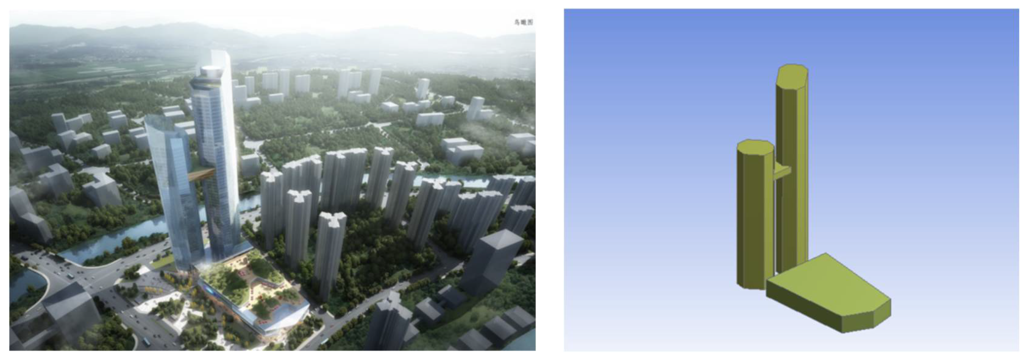
3. Model of the Study

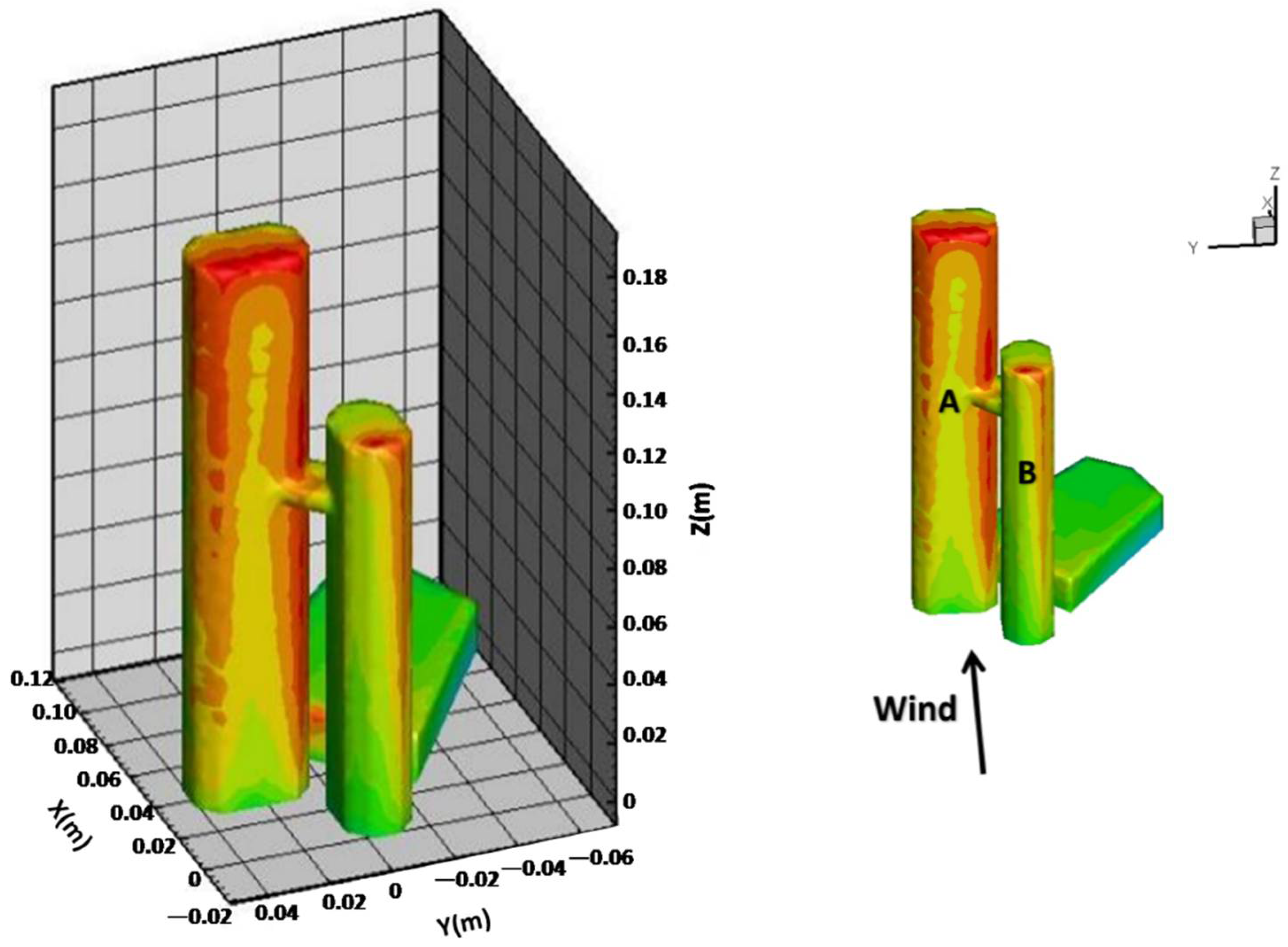
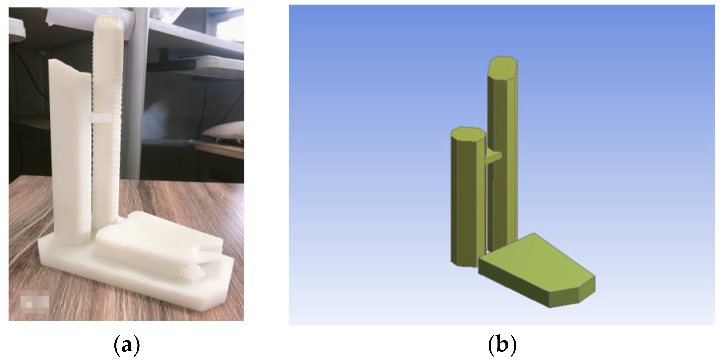
3.1. Model

This paper takes an actual building as an example. The specific building tower A was 270 m high, and tower B was nearly 200 m high, both of which were rigidly connected by a sky-link, with a complex structural system (as shown in Figure 1). In addition, the shortest distance between towers A and B was only 13 m, resulting in complex aerodynamic interference effects between the two towers. In order to compare with the aerodynamic noise wind tunnel experimental results, the numerical simulation model and the wind tunnel model were of the same height, both with a scaling ratio of 1:1500 and a maximum height of 18.5 cm.

The top floor of the original scale building was equipped with complex structures such as aprons, which was simplified into a flat roof during numerical simulation.

3.2. Meshing

Geometry was used to model the computational area in ANSYS, followed by ICEM for meshing and setting boundary conditions. The blockage rate, the ratio of the maximum windward area of the building to the cross-sectional area, is an important indicator to determine whether the dimensions of the computational domain can meet the computational needs. The blockage ratio is required to be less than 3% in numerical simulations [17,18]. Due to the irregularity of the model, the grid was divided into two computational regions, namely inner and outer basins (as shown in Figure 2). The outer basin was 3.6 m long, 1.2 m wide and 1.2 m high, and the inner basin was 0.8 m long, 0.6 m wide and 0.2 m high. The building model was placed inside the inner basin, with the blockage rate of 2%, thus meeting the simulation requirements. The meshing was performed in ICEM software. The unstructured grid was used for the inner basin containing the building due to the irregular structure of the building, and structured grid was used for the outer basin. The grid growth rate was controlled to locally encrypt the grid of the building surface (as shown in Figure 2). In order to obtain more accurate results, the boundary layer of the building model was set. The first grid height of the building model walls was 2 × 10⁻⁴ B (B is the minimum size of the building model after scaling), which was in accordance with the minimum grid size used by Liu et al. [19] in their simulation research on buildings. There were a total of around 4 million meshes in calculation domain under each working condition, with around 2.5 million nodes. The specific settings are shown in Figure 3.

3.3. Boundary Condition Setting

The entry plane of the computational domain was set to velocity inlet. The numerically simulated wind field was similar to the wind field in acoustic wind tunnel experiments, where roughness elements could not be placed to regulate the wind field due to the limited space on the experimental platform and high wind speed. The full cross-sectional mean wind speed was considered the same, and the pulsating wind characteristics of the velocity inlet were defined by the turbulent dissipation ε as well as the turbulence kinetic energy k.

The two physical quantities are defined as:

$$k=\frac{3}{2}{\left(V_u{I}_u\right)}^2$$

(7)

$$\epsilon =\frac{C_u^{\frac{3}{4}}{k}^{\frac{3}{2}}}{l_u}$$

(8)

where V_u is the average wind speed at the entrance of the acoustic wind tunnel experiment, $I_u$ is the turbulence intensity obtained from wind tunnel experiments, and C_u is 0.09. $l_u$ is the turbulence integral length scale. Similarly, in the acoustic wind tunnel, the full-section turbulence was not adjustable and was considered the same, so the default values were used in the turbulence simulation. The specific boundary conditions are shown in Figure 3.

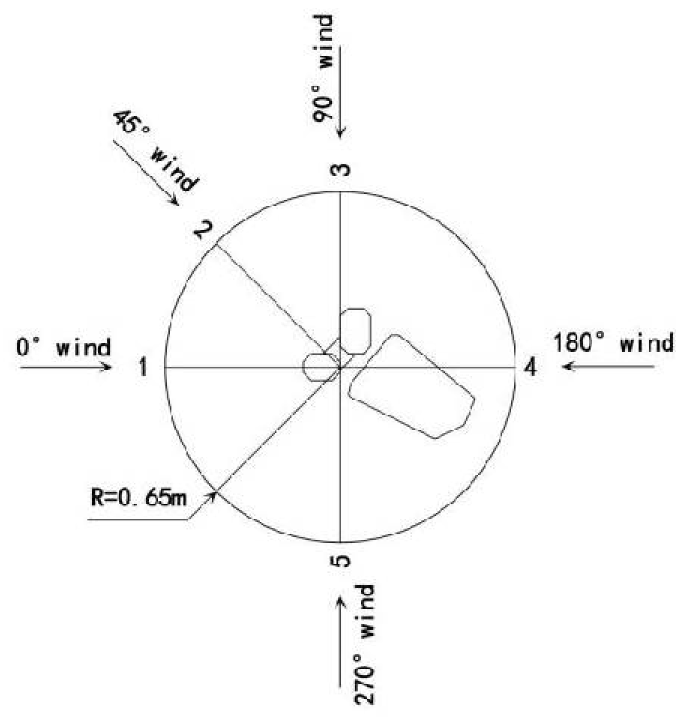
3.4. Noise Monitoring Point Arrangement

According to the wind rose map of Changsha City, the dominant wind directions were 45° and 270°, of which 45° was the most dominant wind direction, so the measuring point diagram is arranged as in Figure 4.

The measuring point was 0.65 m away from the center of the building model, which was the same as the location of the microphone array in the acoustic wind tunnel. It was verified that the location of the measurement points had little effect on the global frequency domain analysis for the same wind angle and the same distance from the model, so they were all arranged on the model centerline in a clockwise direction. There were a total of five measuring points on each floor, each one of which was arranged for each wind direction angle, with five layers evenly arranged in the direction of building height. The layers were 0.04 m away from each other. Among all height measurement points, the height measurement points on the middle floor of the building model were in relatively good agreement with the acoustic wind tunnel experimental results.

3.5. Acoustic Noise Simulation Parameter Setting

The sampling frequency of the acoustic wind tunnel of Wenzhou University was 48,000 Hz. Since the size of the simulation model was the same as that of the experimental model, the time step for simulation was 0.0000208 s, and the sampling frequency was 48,077 Hz, which was basically consistent with the sampling frequency of the acoustic wind tunnel experiment. In addition, six iterations were performed in each time step. The number of computational steps was 10,000, and the computation was considered converged when each residual was below 10⁻⁵. The sound velocity was 340 m/s, the reference sound pressure was 2 × 10⁻⁵ Pa, and the sound source area was the surface of the building model. To calculate the spectrum of the measured sound field at the measuring point, the corresponding sound source area of the building model needed to be activated.

4. Analysis of the Calculated Sound Pressure Intensity Distribution Cloud Map

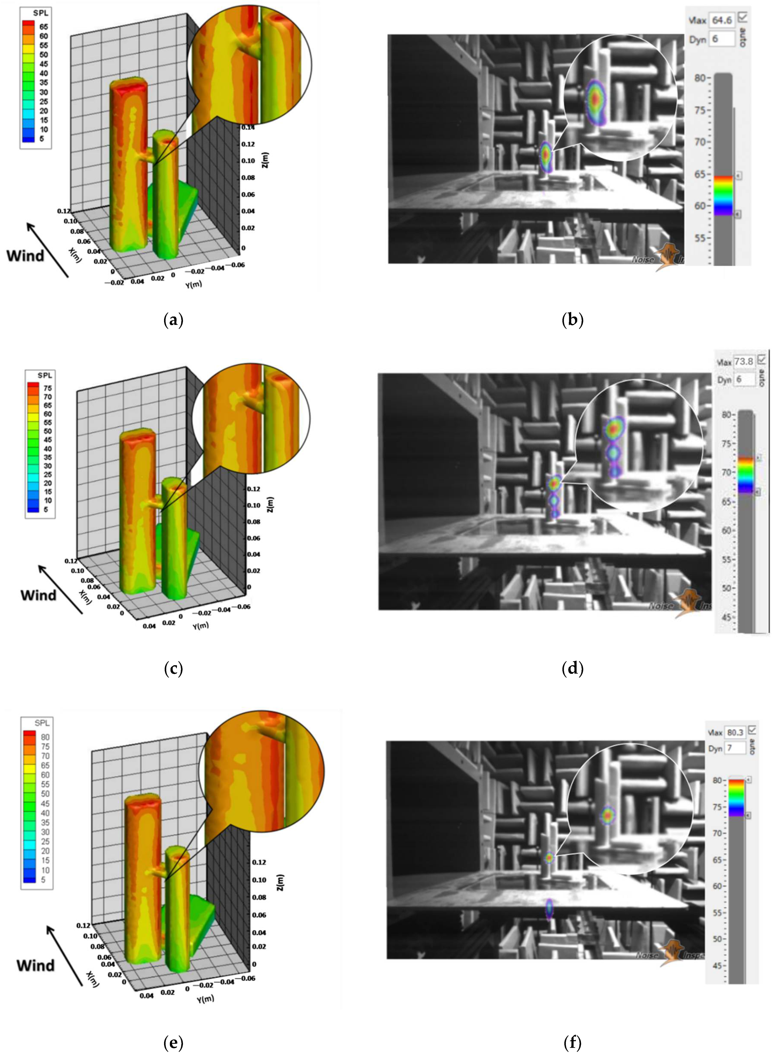
4.1. Analysis of Simulation Results of Sound Pressure Intensity on Building Surfaces

The simulated sound pressure level cloud map on the surface of the building model with an inlet wind speed of 25 m/s at 0° wind angle was taken as an example for analysis.

Sound pressure level is generally used to reflect noise intensity. The wind flowed from the negative half-axis of the X-axis to the positive half-axis under all working conditions. It can be seen from Figure 5 that the distribution of sound pressure intensity at various points on the surface of the building model could be obtained by numerical simulation, and surfaces A and B were windward at a wind angle of 0°. The sound pressure level on the windward side of the building, the gap between the two buildings and the edge of the building was higher, which conformed to the conjecture that the greater the airflow disturbance, the stronger the aerodynamic noise intensity radiation. The location of the localized noise source is in the darkest red area in the cloud map.

The color contrast of the cloud map was adjusted as follows.

It can be seen from Figure 6 that the area of maximum sound pressure level on the surface of the building model was highlighted by adjusting the color contrast of the cloud map display, the area of maximum sound pressure level on the surface of the building model, thus achieving the purpose of locating noise source.

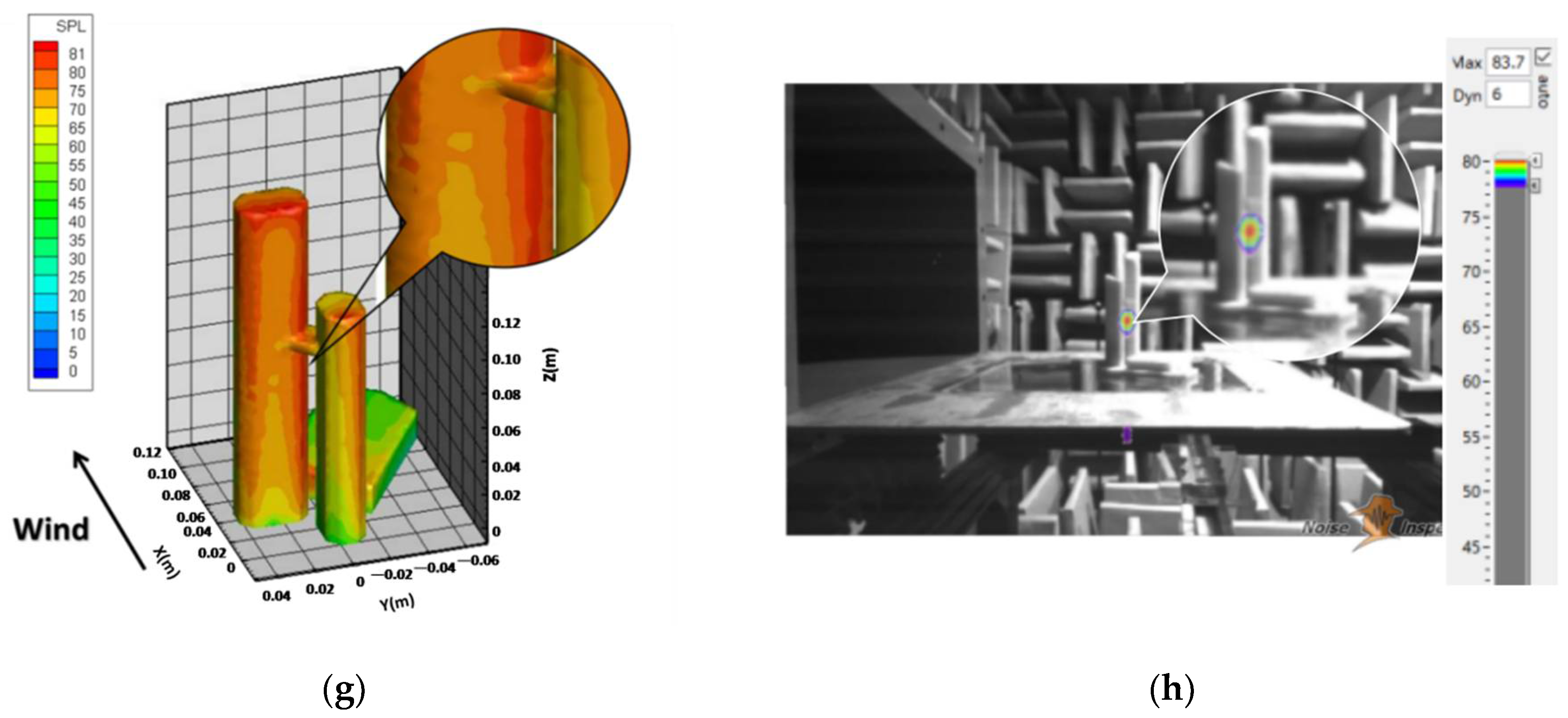
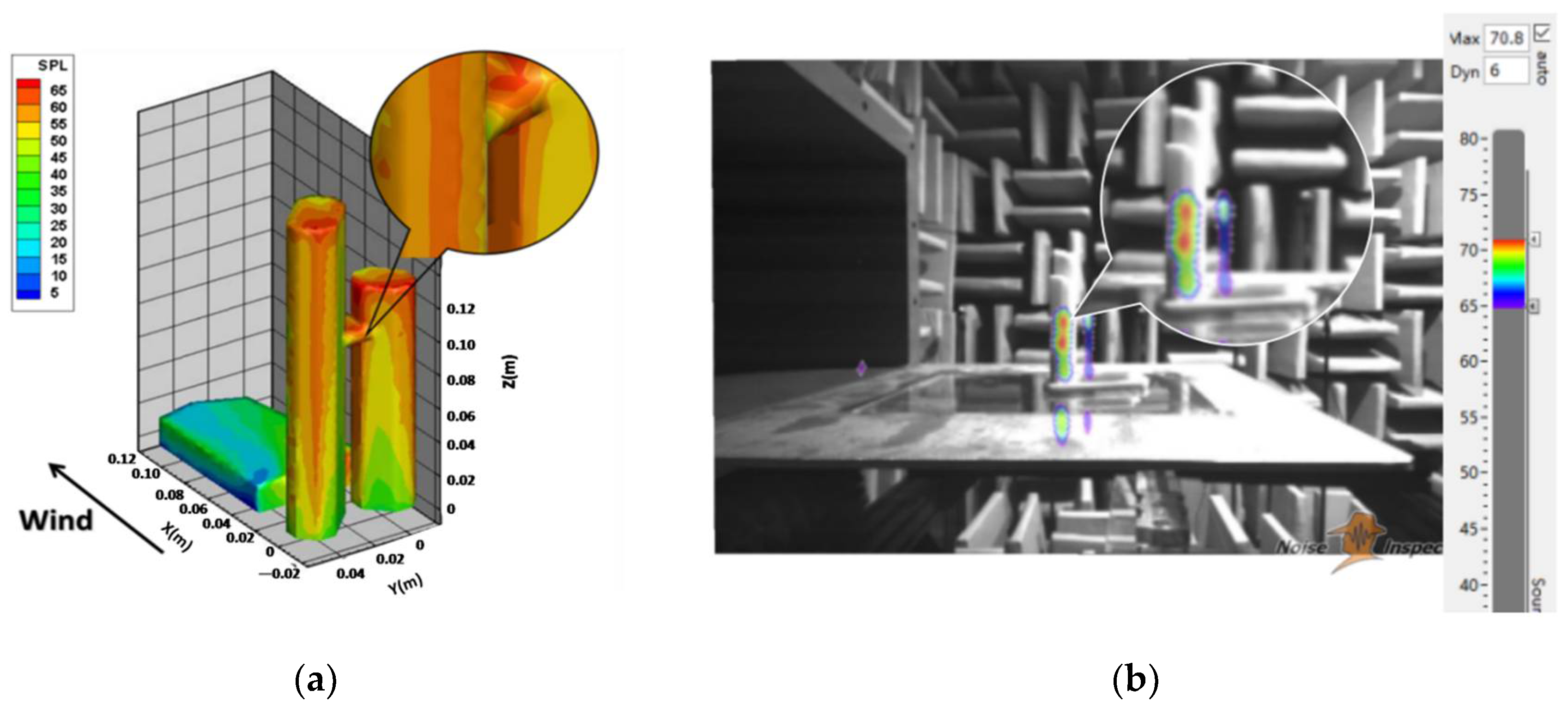
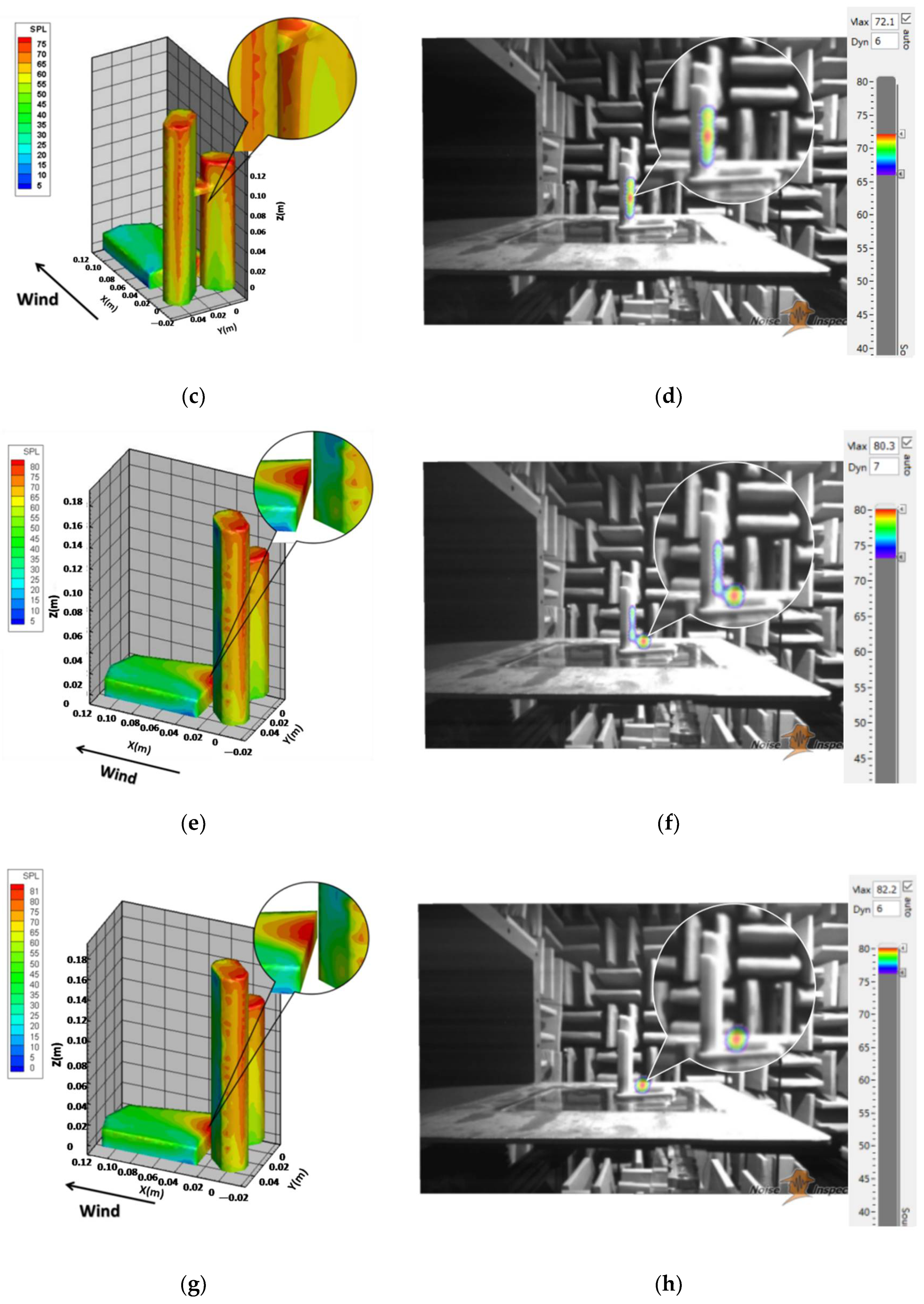
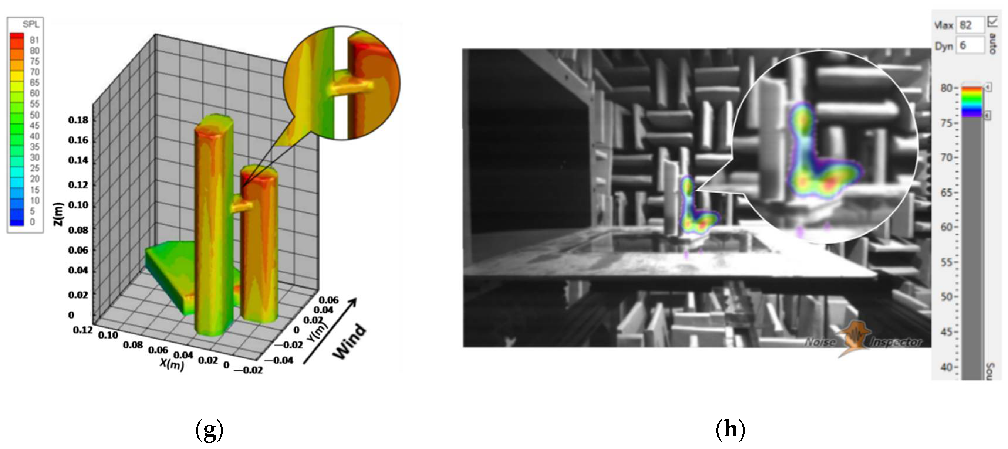
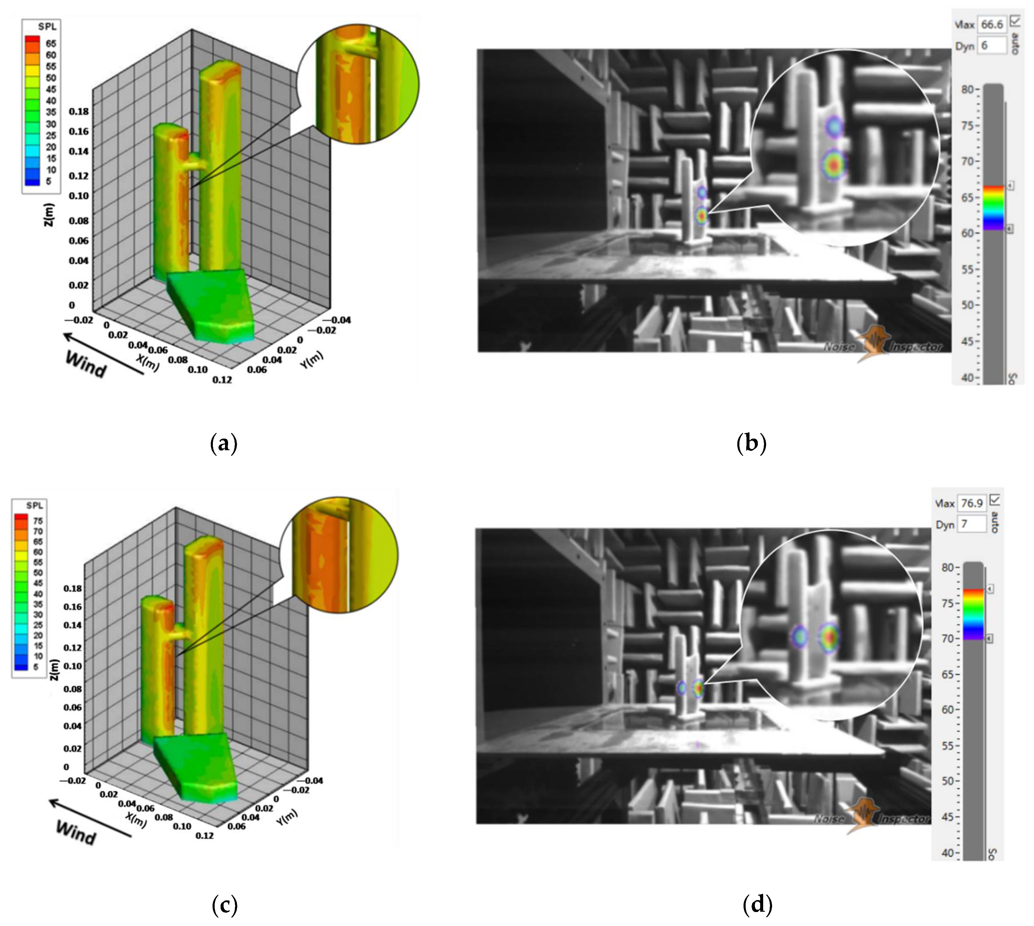
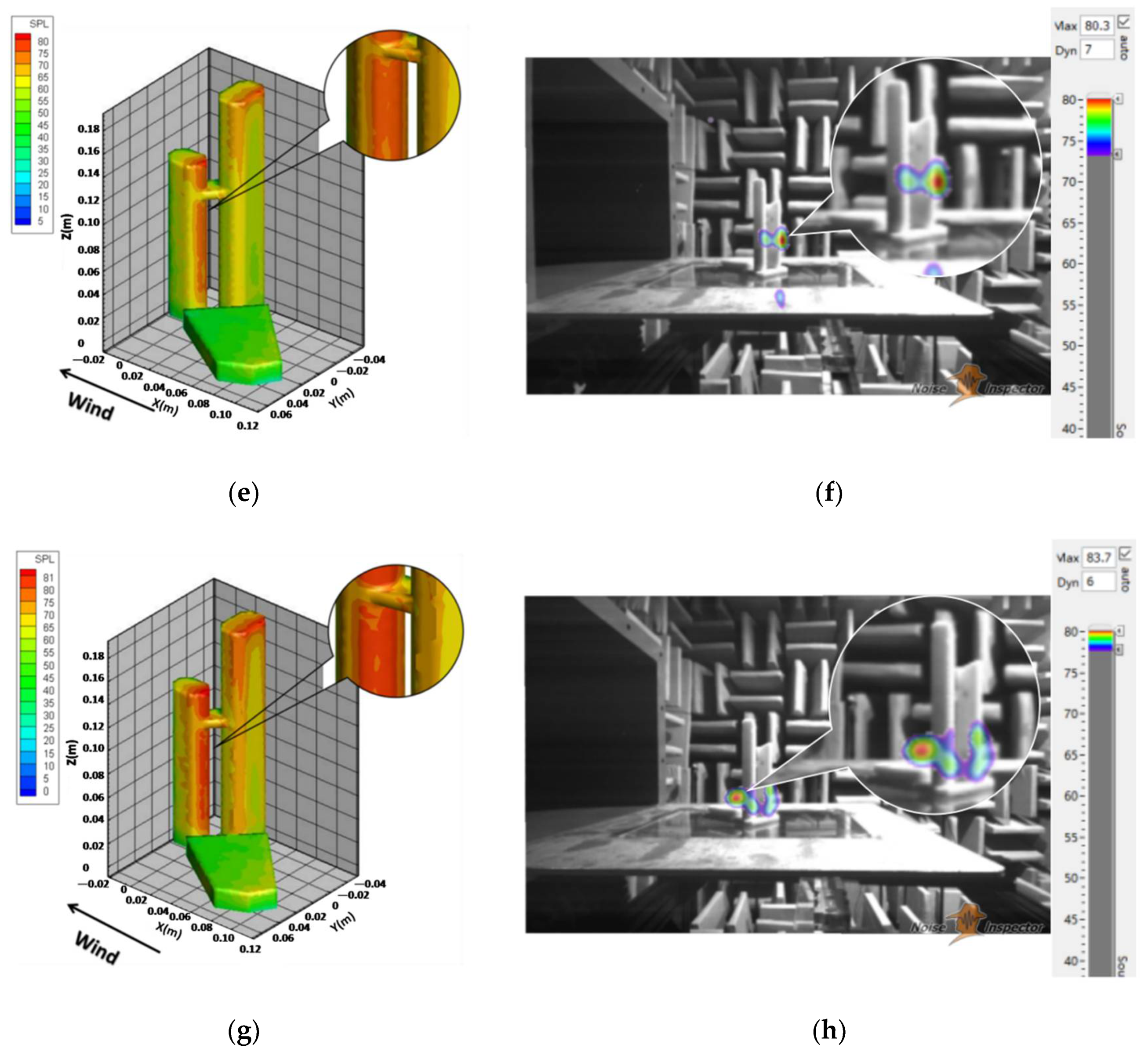
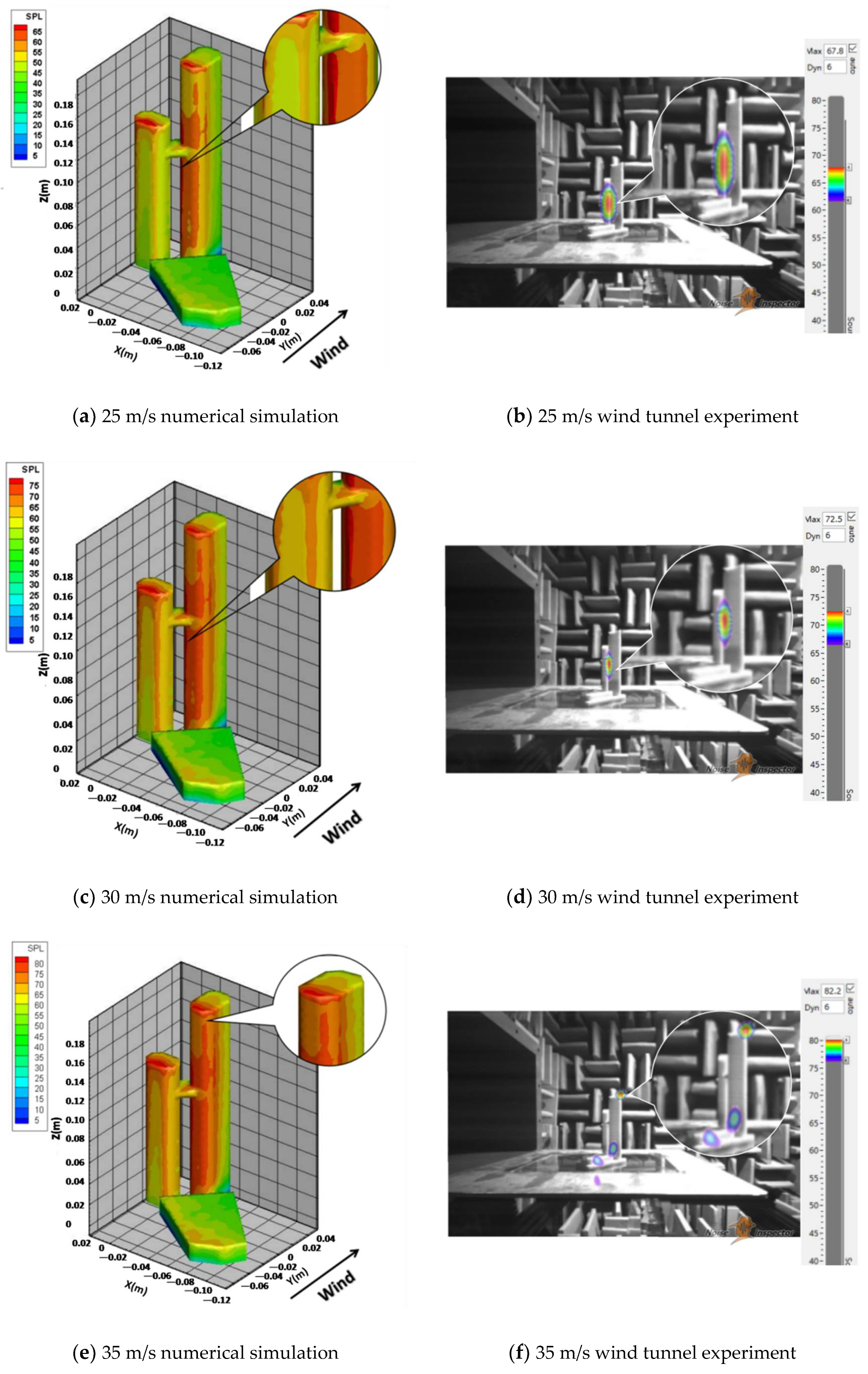
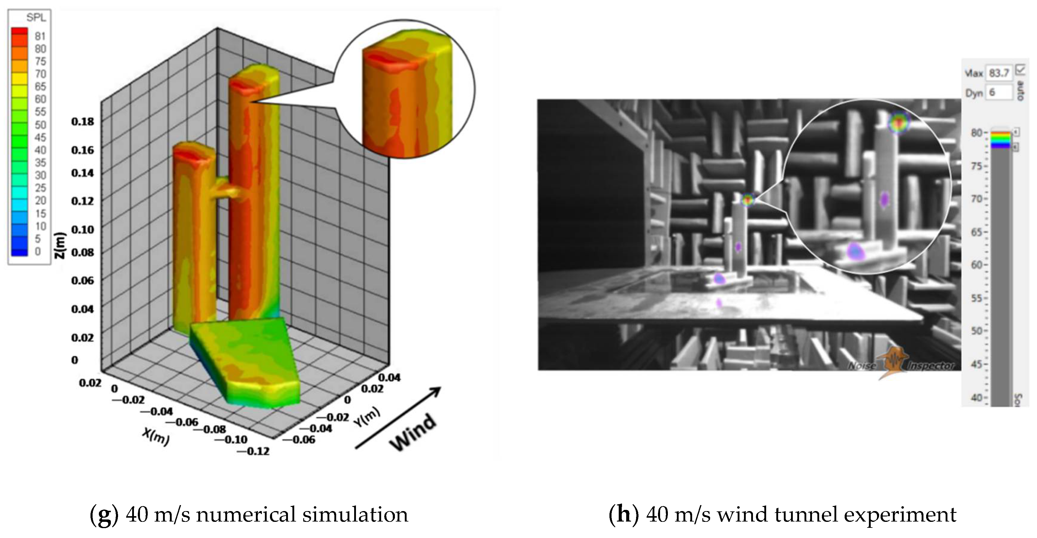
4.2. Comparison Results between Simulated and Experimental Noise Source Localization Cloud Maps under Each Working Condition

It can be seen from Figure 7 that the numerically simulated sound source localization at the wind angle of 0° at each wind speed was in good agreement with the acoustic wind tunnel experimental results, as was the sound pressure level amplitude of the sound source.

As can be seen from Figure 8, the numerically simulated sound source localization at the wind angle of 45° at each wind speed was in relatively good agreement with the acoustic wind tunnel experimental results, as was the sound pressure level amplitude of the sound source.

From Figure 9, it can be seen that the numerically simulated sound source localization at the wind angle of 90° at each wind speed was consistent with the acoustic wind tunnel experimental results in the height direction, as was the sound pressure level amplitude of the sound source.

As can be seen from Figure 10, at the wind angle of 180°, the numerical simulation and the location of the local sound source in the acoustic wind tunnel corresponded to each other in the height direction at each wind speed but with slight difference. However, the localized sound pressure level magnitude was consistent.

As can be seen from Figure 11, the numerically simulated sound source localization at low wind speed at the wind angle of 270° was in good agreement with the acoustic wind tunnel experimental results. The deviation of the upper localized sound source location under the working conditions of 35 m/s and 40 m/s was caused by the complex modeling of the apron in the upper part of the building, which was simplified in the numerical simulation by reducing the apron to a regular solid figure, but 3D printing technology was adopted in the wind tunnel experimental model to reproduce the external contour of the complex structure at the top. The total height of the two models was the same, whose appearances were identical except for the detailed structure as well as the top layer structure (as shown in Figure 12). In addition, the sound pressure level amplitude of the sound source was in good agreement.

Summing up the results, the numerical simulation and acoustic wind tunnel experimental results under the working conditions of 0°, 45° and 270° were in good agreement in terms of locating the sound source. The height was also in good agreement between the numerical simulation and the acoustic wind tunnel experiment for locating the sound source under the working conditions of 90° and 180°, but there was a slight difference between the front and rear positions. This is because for stationary sound sources, although the microphone array [20,21,22,23] can discriminate incoherent sources based on the traditional beamforming algorithm of delay superposition, the spatial resolution is relatively low, and the building model in this paper is relatively complex compared to the research model in the field of aerospace and vehicle engineering. Furthermore, there is a gap in the middle of the buildings that is not easily monitored by the microphone array, and the main airflow disturbance is generated in the gap. In addition, there were various unavoidable installation deviations when the microphone array was installed, and such installation deviations resulted in the sound source localization errors [24,25]. The numerical simulation results on the top layer of the experimental model had no effect on the spatial distribution of noise intensity and no significant effect on the localization of noise sources, except for a slight difference in the localization cloud map at a higher wind speed of 270°. The simplification of the simulation model relative to the experimental model can be considered to be within a reasonable range. The numerical simulation and the acoustic wind tunnel in locating the sound pressure level of the sound source under all working conditions was also consistent, so was the sound pressure level amplitude of the sound source.

Therefore, the numerical simulation method combining large-eddy simulation and FW-H proposed in this paper can reasonably simulate the aerodynamic noise distribution on the surface of the building and locate the noise source. Furthermore, the sound pressure level spectrum was further analyzed to improve the parameter settings of the numerical simulation details.

5. Analysis of Sound Pressure Level Spectrum in Acoustic Wind Tunnel Experiment

The acoustic wind tunnel experimental noise sound source was acquired by microphone array, which was used to identify the sound source wavefront in the sound field with the help of a certain number of calibrated microphones. The acoustic wind tunnel acquisition of the sound pressure time course was processed using the software that came with the microphone array. The principle was to process data using the beamforming method [26], where the signal focused on the sound source. After adjusting the time at which the sound travelled from the source to the microphone, all signals would be in the same phase [27,28,29], all of which would be summed up, as shown in Figure 13. As can be seen from the figure, as the value increased, the sound localization image tended to be red. A sharp peak emerged in the sound pressure level spectrum.

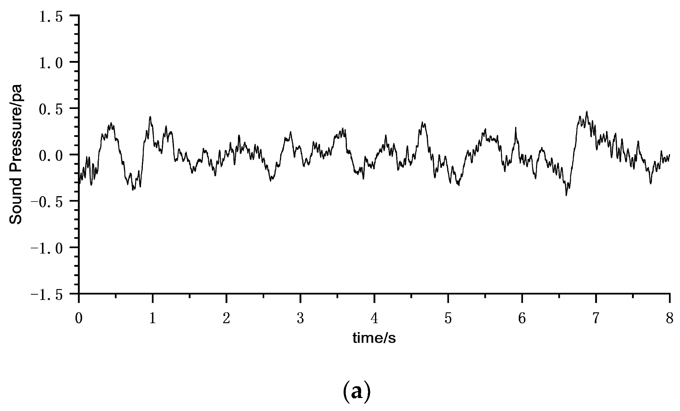
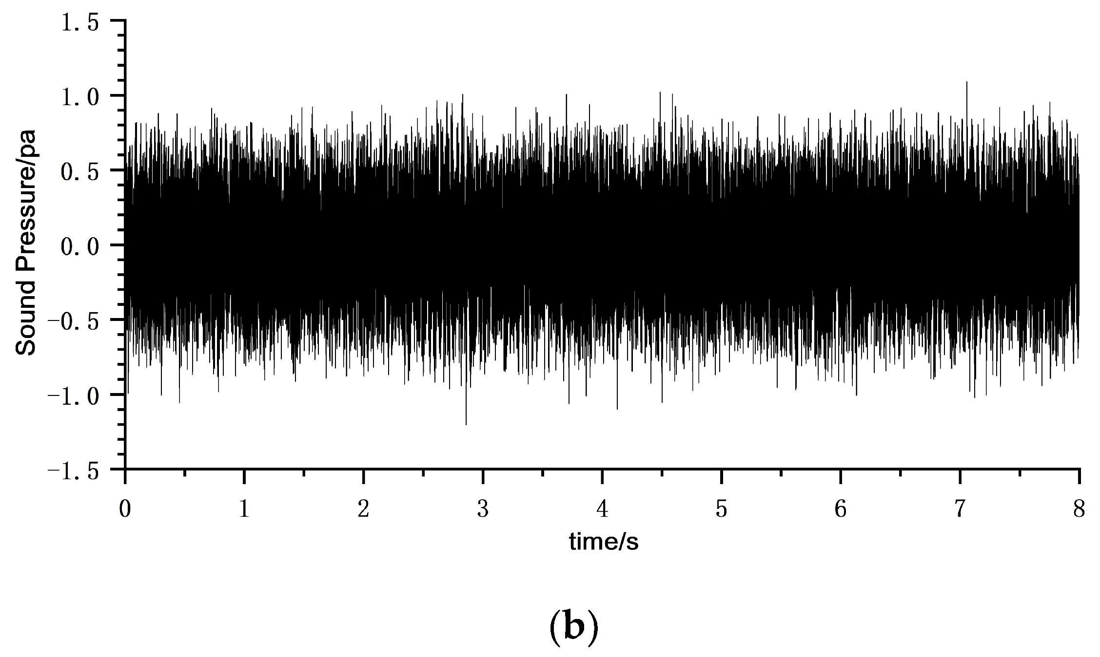
5.1. Time Domain Analysis

After the model was placed in the wind tunnel, the new noise generated by the building model was added to the time course of the original background noise at the same wind speed. Figure 14 shows the time courses of sound pressure before and after the model was placed at the wind speed of 30 m/s and the wind direction angle of 0°.

The above figure shows that in terms of amplitude, after placing the model in Figure 14b, the overall amplitude of sound pressure increased relative to the background sound pressure in Figure 14a, which was attributed to the background noise sound pressure superimposed on the building surface aerodynamic noise. In terms of pulsation frequency, after placing the model in Figure 14b, the sound pressure pulsation frequency increased significantly in the high-frequency band relative to the background sound pressure in Figure 14a. Therefore, it can be assumed that the pulsation sound pressure in the high-frequency band was mainly influenced by the aerodynamic noise on the surface of the building model.

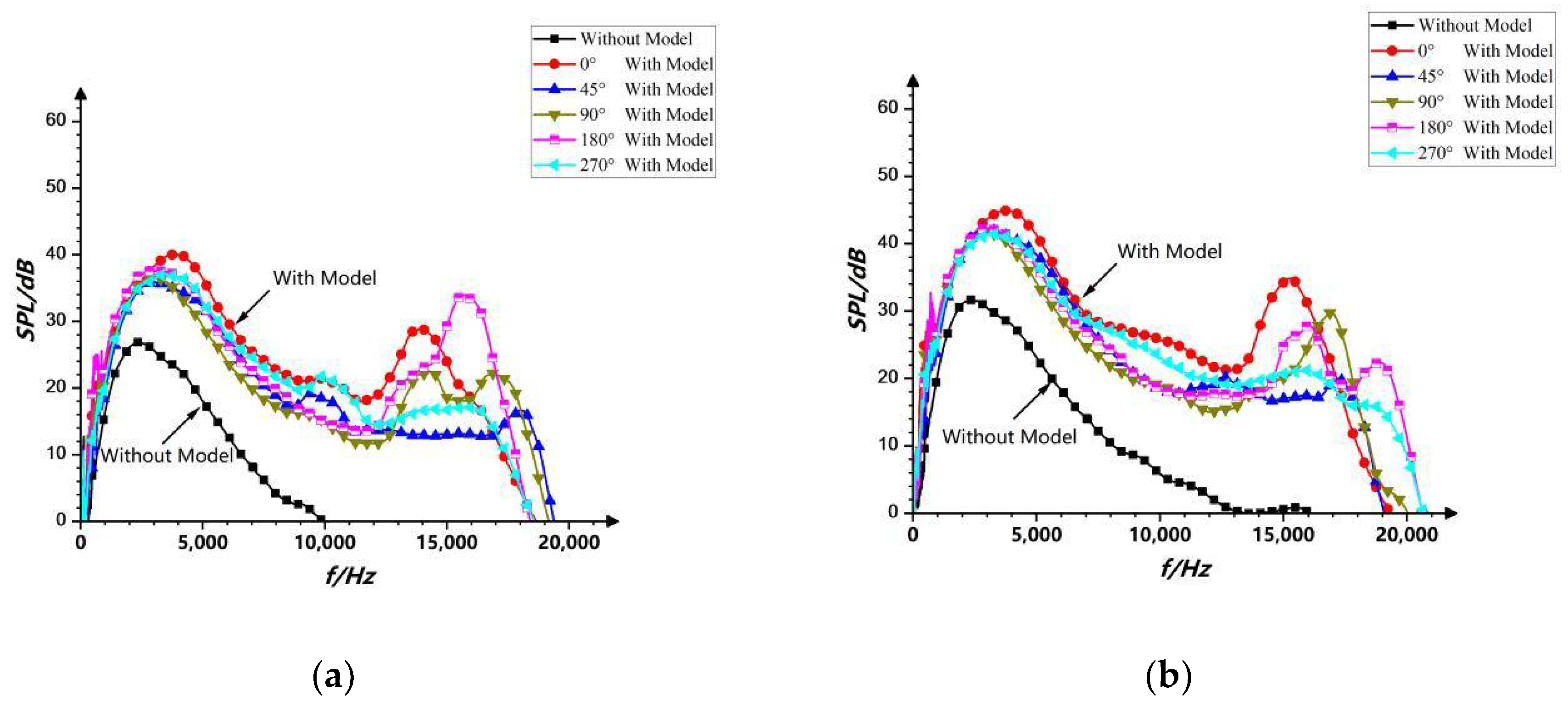
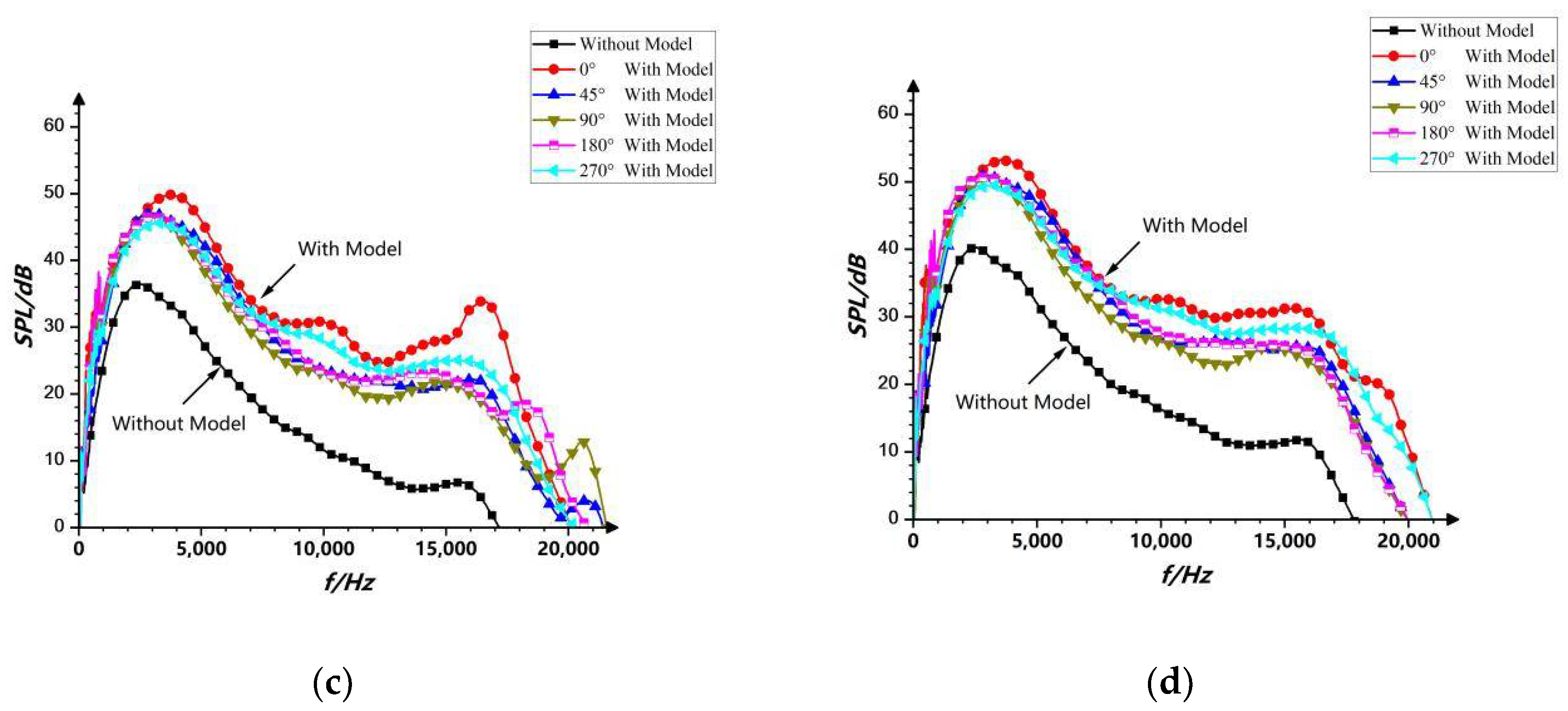
5.2. Frequency Domain Analysis

The fast Fourier transform was performed on the sound pressure time course to obtain the sound pressure level spectra under each working condition, which were then sliding averaged [30,31,32]. The finite adjacent values of the experimental data with and without the model were respectively averaged to suppress the influence of random errors on the experimental results, as shown in Figure 15.

At the same wind speed, no obvious pattern was observed for the variation law of wind angle in the SPL spectra after the model was put into the wind tunnel. However, as wind speed increased from 25 m/s to 35 m/s, spike-like peaks in the high-frequency band of the sound pressure level spectrum gradually shifted to higher frequencies, and when wind speed further increased to 40 m/s, no obvious spike-like peaks emerged in the high-frequency band under most working conditions.

It can be seen from the figure that the sound pressure level spectrum without the model had relatively smaller values than the overall sound pressure level spectrum with the model, which was consistent with time course analysis results. Taken together, in the sound pressure level spectrum analysis, the greater the difference between the background noise and the noise spectrum line after placing the model, the stronger the noise generated by the building model. Then, the difference between the sound pressure level with the model and the sound pressure level with background noise for each working condition at the same frequency could be used as the basis for the macroscopic judgment of the size of the aerodynamic noise radiated from the surface of the building model. As can also be seen from Figure 15, after placing the model in the wind tunnel, the sound pressure level in the high-frequency band changed even more dramatically, so the aerodynamic noise generated by the building model was mostly in the high-frequency band, which was consistent with time domain analysis results.

At the same wind speed, peaks emerged in the frequency band of 0–5000 Hz of the spectrogram regardless of whether model was placed. Furthermore, judging from the image sound pressure level difference, the difference in the low-frequency band is lower than that in the high-frequency band, so it can be assumed that the peak in the low-frequency band is more affected by the background noise.

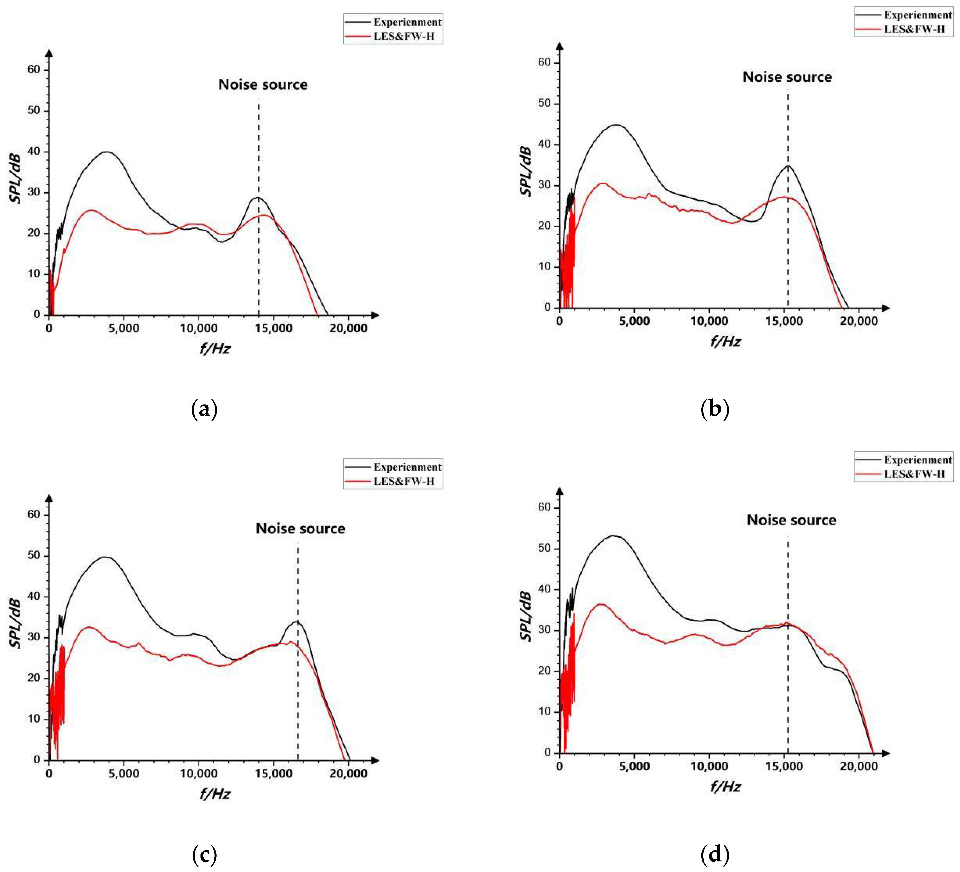
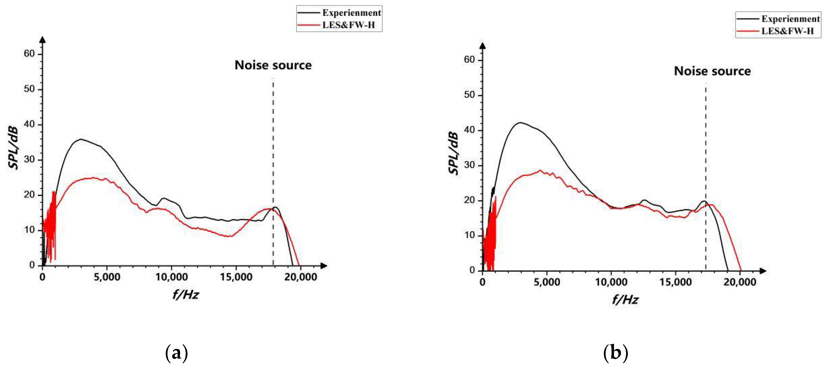
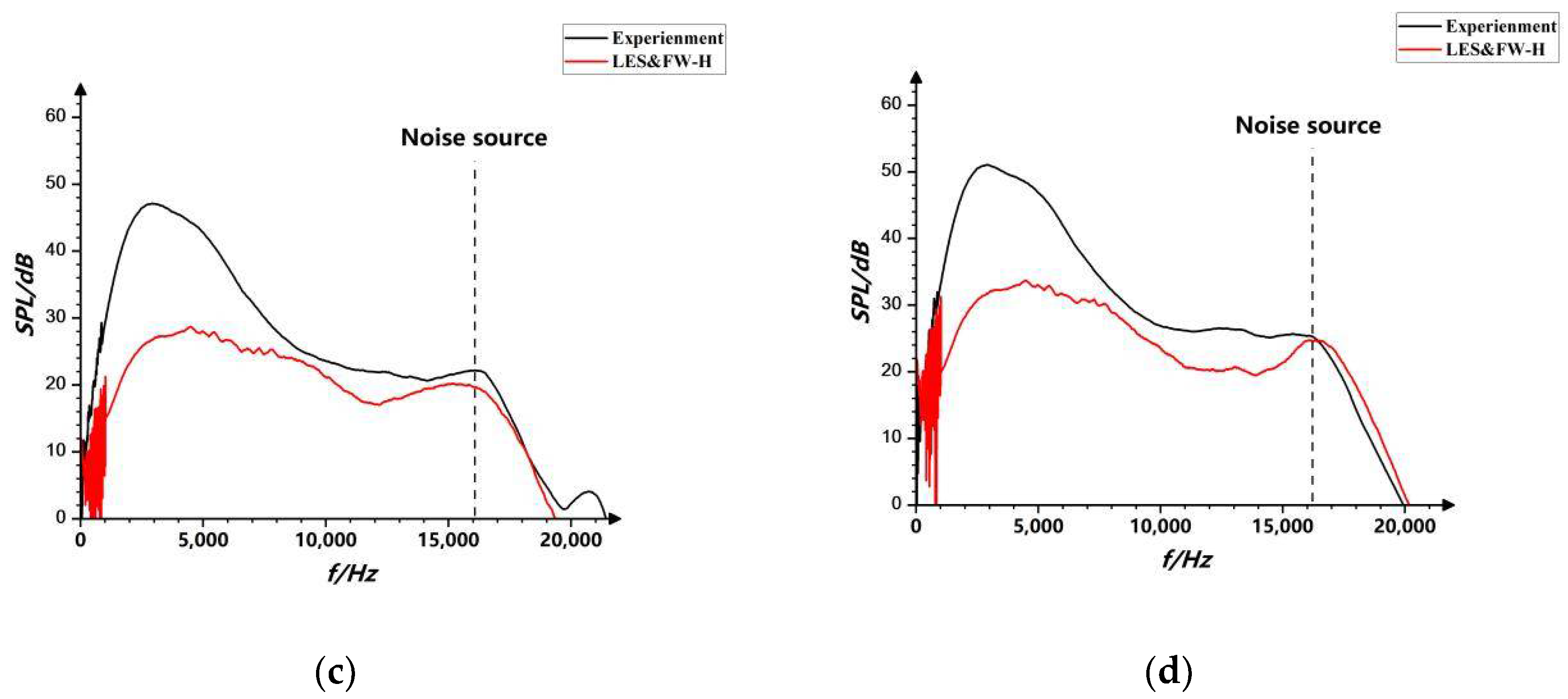
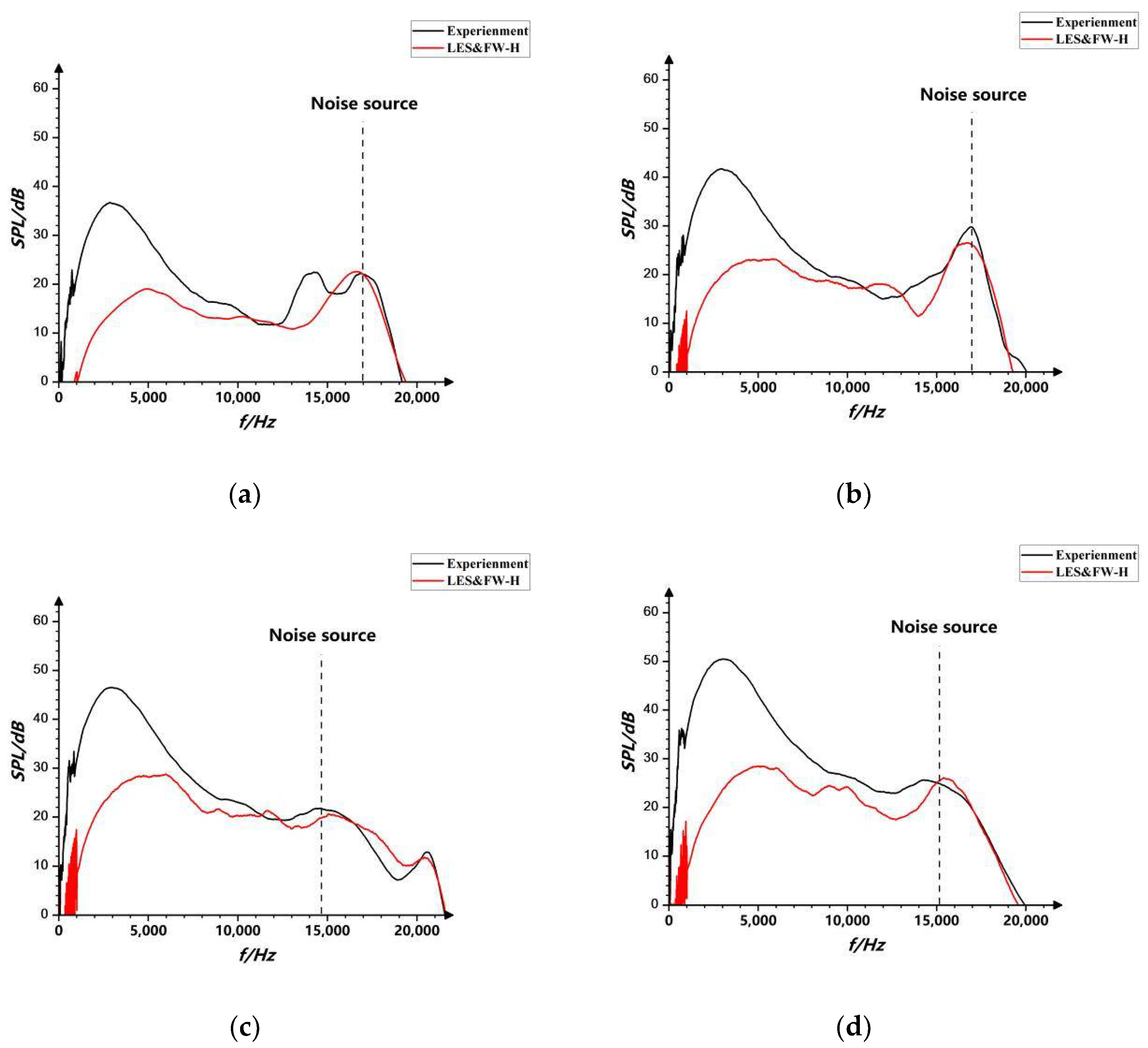
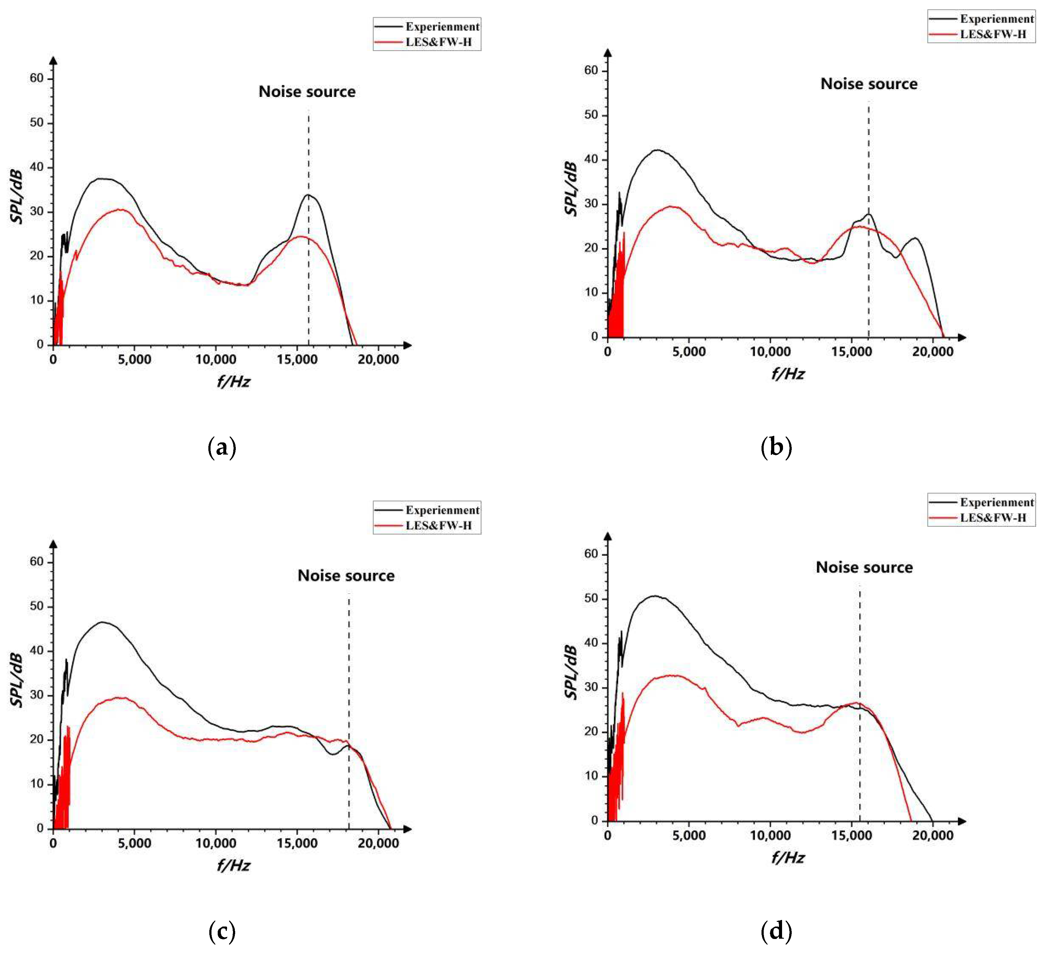
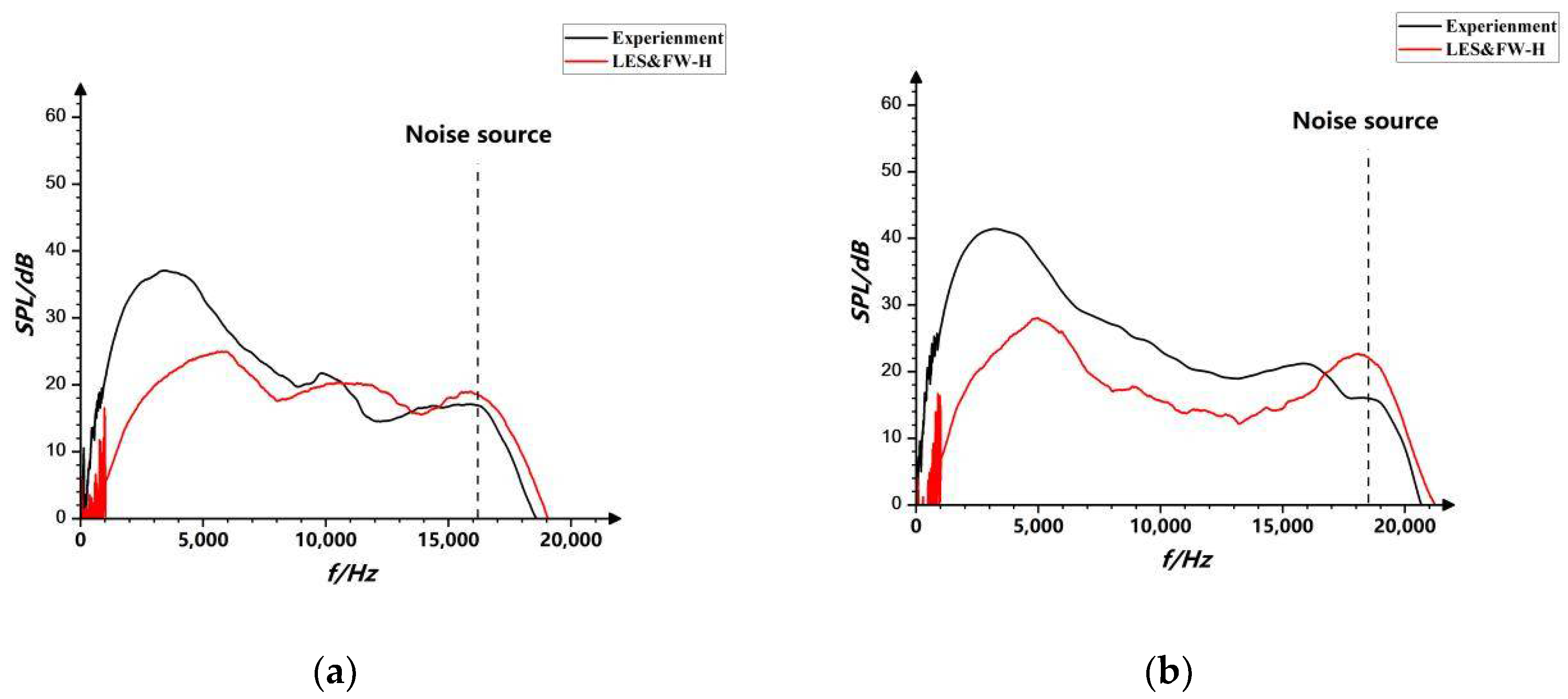
6. Comparison of Sound Pressure Level Spectrum between Numerical Simulation and Wind Tunnel Experiment

The time course of sound pressure pulsation was collected, and the sound pressure level spectrum data of each point was obtained by fast Fourier transform (FFT) and then compared with the acoustic wind tunnel experimental results for verification, as shown in Figure 16, Figure 17, Figure 18, Figure 19 and Figure 20.

The numerical simulation results of four wind speeds at five angles indicate that the numerical simulation and the wind tunnel experimental results are in good agreement in the middle- and high-frequency bands in terms of sound pressure level spectrum but with a slight difference in the low-frequency band of 0–5000 Hz. According to the frequency–time waterfall diagram of the acoustic wind tunnel experiment, the peak value of the acoustic wind tunnel SPL spectrum in the high-frequency band was also the frequency of the sound source, indicating that the frequency of noise source in the SPL spectrum was in good agreement between the numerical simulation and the acoustic wind tunnel experiment.

As mentioned earlier, acoustic wind tunnel experimental measurement in the low-frequency band was greatly influenced by the aerodynamic background noise generated by wind tunnel outlet, experimental platform, etc. However, only the ideal acoustic environment unaffected by background noise was considered during numerical simulation. Therefore, there was a reasonable difference between the numerical simulation results and the acoustic wind tunnel experimental results in the low-frequency band. In summary, the results of the numerical simulation method combining large-eddy simulation and FW-H were consistent with acoustic wind tunnel experimental results, which, hence, can be used to evaluate wind-induced acoustic environment in high-rise buildings.

7. Conclusions

Comparing the results of the numerical simulation combining large-eddy simulation and the FW-H equation for determining the aerodynamic noise of high-rise buildings with the acoustic wind tunnel experimental results, we can make conclusions as follows:

(1)

The numerical simulation of the aerodynamic noise of the high-rise building is in good agreement with the localization results for noise sources in an acoustic wind tunnel, and thus, a noise source on the surface of a high-rise building can be located by numerical simulation.

(2)

Because of limited experimental conditions, wind tunnel experimental results in the low-frequency band are greatly influenced by background noise, resulting in the deviation of sound pressure level spectrum from the simulated results in the low-frequency band.

(3)

The numerical simulation results are in good agreement with the acoustic wind tunnel experimental results in the middle- and high-frequency bands, which are more significantly influenced by the aerodynamic noise radiated from the surface of the building model.

(4)

The numerical simulation method can be used to calculate aerodynamic noise intensity at various points on the surfaces of high-rise buildings and reasonably predict and evaluate the influence of wind-induced aerodynamic noise on the environment.

(5)

The numerical simulation method can reproduce the results of acoustic wind tunnel experiments with high accuracy.

This paper can provide a theoretical basis for research on the localization of aerodynamic noise radiation sources in the full-scale model and the methods for controlling aerodynamic noise on the surfaces of high-rise buildings. The combination of numerical simulation and acoustic wind tunnel experiments was used for the first time in the study of aerodynamic noise in high-rise buildings. The method of numerical simulation for locating noise sources was first applied to the study of locating noise sources on the surfaces of high-rise buildings. Numerical simulation research on the surface aerodynamic noise of building models can optimize the appearance of high-rise buildings in the architectural design stage and locate the existing high-rise building surface aerodynamic noise sources, allowing for more accurate and effective local noise reduction research processing, saving resources, reducing urban environmental noise pollution, and optimizing the living environment.

References

1. Tam, C.K.W. Discrete tones of isolated airfoils. J. Acoust. Soc. Am. 1974, 55, 1173–1177. [Google Scholar] [CrossRef]
2. Nakano, T.; Kim, H.J.; Lee, S.; Fujisawa, N.; Takagi, Y. A study on discrete frequency noise from a symmetrical airfoil in a uniform flow. In Proceedings of the 5th JSME-KSME Fluids Eng conference, Nagoya, Japan, 17–21 November 2002. [Google Scholar]
3. Chanthanasaro, T.; Boonyasiriwat, C. Numerical Study on Characteristics of Sound and Wake Generated by Flow past Triangular Cylinder at Various Incident Angles. J. Phys. Conf. Ser. 2021, 1719, 12034. [Google Scholar] [CrossRef]
4. Wang, M.; Moin, P. Computer of trailing-edge flow and noise using large-eddy simulation. AIAA J. 2015, 38, 2201–2209. [Google Scholar] [CrossRef]
5. Mo, J.O.; Lee, Y.H. Numerical simulation for prediction of aerodynamic noise characteristics on a HAWT of NREL phase VI. J. Mech. Sci. Technol. 2011, 25, 1341–1349. [Google Scholar] [CrossRef]
6. Angelino, M.; Xia, H.; Page, G.J. Influence of grid resolution on the spectral characteristics of noise radiated from turbulent jets: Sound pressure fields and their decomposition—ScienceDirect. Comput. Fluids 2020, 196, 104343. [Google Scholar] [CrossRef]
7. Liu, B.; Guo, J.S.; Zhang, X.L. Research on outdoor aerodynamic noise of super high-rise buildings based on CFD technology. Archit. Tech. 2011, 3, 164–166. [Google Scholar]
8. Au, T.; Zhang, Y.H.; Xu, W.; Tan, J. Pneumatic noise simulation and its application in Hengqin Development Building. In Proceedings of the 2014 Annual Meeting of the Building Structure Branch of the Architectural Society of China and the Twenty-third National Academic Exchange Conference on Tall Building Structures, Ed. of Building Structures, Guangzhou, China, 19 November 2014; pp. 1–4. Available online: https://d.wanfangdata.com.cn/conference/8848250 (accessed on 14 September 2022).
9. Zhu, Z.; Deng, Y. Large Eddy Simulation of Aerodynamic Noise Field in Super Tall Buildings. J. Southwest Jiaotong Univ. 2019, 54, 748–756. [Google Scholar]
10. Aihara, A.; Bolin, K.; Goude, A.; Bernhoff, H. Aeroacoustic noise prediction of a vertical axis wind turbine using large eddy simulation. Int. J. Aeroacoust. 2021, 20, 959–978. [Google Scholar] [CrossRef]
11. Hamiga, W.M.; Ciesielka, W.B. Numerical Analysis of Aeroacoustic Phenomena Generated by Heterogeneous Column of Vehicles. Energies 2022, 15, 4669. [Google Scholar] [CrossRef]
12. Karthik, K.; Vishnu, M.; Vengadesan, S.; Bhattacharyya, S.K. Optimization of bluff bodies for aerodynamic drag and sound reduction using CFD analysis. J. Wind Eng. Ind. Aerodyn. 2018, 174, 133–140. [Google Scholar] [CrossRef]
13. Chen, N.S.; Liu, H.R.; Liu, Q.; Zhao, X.Y.; Wang, Y.G. Effects and mechanisms of LES and DDES method on airfoil self-noise prediction at low to moderate Reynolds numbers. AIP Adv. 2021, 11, 025232. [Google Scholar] [CrossRef]
14. Smagorinsky, J.S.; Smagorinsky, J. General Circulation Experiments with the Primitive Equations. Mon. Weather Rev. 1963, 91, 99–164. [Google Scholar] [CrossRef]
15. Lighthill, M.J. On sound generated aerodynamically Ⅱ. Turbulence as a source of sound. Proc. R. Soc. Lond. 1954, 222, 1–32. [Google Scholar]
16. Illiams, J.E.F.; Hawkings, D.L. Sound generation by turbulence and surfaces in arbitrary motion. Philosophical Transactions of the Royal Society of London Series A. Math. Phys. Sci. 1969, 264, 321–342. [Google Scholar]
17. Blocken, B.J.E. Computational Fluid Dynamics for urban physics: Importance, scales, possibilities, limitations and ten tips and tricks towards accurate and reliable simulations. Build. Environ. 2015, 91, 219–245. [Google Scholar] [CrossRef]
18. Hunt, A. Wind-tunnel measurements of surface pressures on cubic building models at several scales. J. Wind Eng. Ind. Aerodyn. 1982, 10, 137–163. [Google Scholar] [CrossRef]
19. Liu, J.; Niu, J.C.F.D. simulation of the wind environment around an isolated high-rise building: An evaluation of SRANS, LES and DES models. Build. Environ. 2016, 96, 91–106. [Google Scholar] [CrossRef]
20. Dougherty, R.P. Beamforming in acoustic testing. In Aeroacoustic Measurements; Springer: Berlin/Heidelberg, Germany, 2002; pp. 62–97. [Google Scholar]
21. Underbrink, J.R. Aeroacoustic phased array testing in low speed wind tunnels. In Aeroacoustic Measurements; Springer: Berlin/Heidelberg, Germany, 2002; pp. 98–217. [Google Scholar]
22. Liu, Y.; Quayle, A.R.; Dowling, A.P.; Sijtsma, P. Beamforming correction for dipole measurement using two-dimensional microphone arrays. J. Acoust. Soc. Am. 2008, 124, 182–191. [Google Scholar] [CrossRef]
23. Soderman, P.T.; Noble, S.C. Directional Microphone Array for Acoustic Studies of Wind Tunnel Models. J. Aircr. 1975, 12, 168–173. [Google Scholar] [CrossRef]
24. Bao, H.; Yang, M.; Ma, W. Rotating sound source localization error caused by microphone array installation deviation. J. Aerosp. Power 2019, 34, 1708–1716. [Google Scholar]
25. Brooks, T.; Humphreys, W. Effect of Directional Array Size On The Measurement of Airframe Noise Components. AIAA Pap. 1999, 99–1958. [Google Scholar] [CrossRef]
26. Gu, G.; Zhu, B. Aeroacoustic wind tunnel background noise testing and spectrum analysis. Noise Vib. Control. 2011, 31, 156–158+162. [Google Scholar]
27. Howell, G.P.; Bradley, A.J. De-dopplerization and acoustic imaging of aircraft flyover Noise measurement. J. Sound Vib. 1986, 105, 151–167. [Google Scholar] [CrossRef]
28. Brooks, T.F.; Marcolini, M.A.; Pope, D.S. A directional array approacch for the measurement of rotor noise source distributions with controlled spatial resolution. J. Sound Vib. 1987, 112, 192–197. [Google Scholar] [CrossRef]
29. Gramann, R.A.; Mocio, J.W. Aero-acoustic measurements in wind tunnels using conventional adaptive beamforming methods. AIAA Pap. 1993, 93–4341. [Google Scholar] [CrossRef]
30. Pei, Y.; Guo, M. The basic principle and application of sliding average method. J. Gun Launch Control 2001, 1, 21–23. [Google Scholar]
31. Maruta, Y.; Minorikawa, G. Background Noise in Measuring Section of Low-Noise Acoustic Wind Tunnels: 1st Report, Analysis of Background Noise Sources in Measuring Section Yoshiyuki Maruta, Gaku Minorikawa. Trans. Jpn. Soc. Mech. Eng. Ser. B 1995, 61, 3741–3748. [Google Scholar] [CrossRef] [Green Version]
32. Duell, E.; Yen, J.; Walter, J.; Arnette, S. Boundary layer noise in aeroacoustic wind tunnels. In Proceedings of the 42nd AIAA Aerospace Sciences Conference, Reno, NV, USA, 5–8 January 2004; p. 1028. [Google Scholar]
Figure 1. Aerial view of the building.
Applsci 12 09446 g001
Figure 2. Computational domain meshing partitioning.
Applsci 12 09446 g002
Figure 3. Computational domain mesh.
Applsci 12 09446 g003
Figure 4. Measurement point layout.
Applsci 12 09446 g004
Figure 5. Sound pressure level nephogram.
Applsci 12 09446 g005
Figure 6. Noise source localization.
Applsci 12 09446 g006
Figure 7. Comparison of experimental and simulated sound source localization at the wind angle of 0°. (a) 25 m/s numerical simulation; (b) 25 m/s wind tunnel experiment; (c) 30 m/s numerical simulation; (d) 30 m/s wind tunnel experiment; (e) 35 m/s numerical simulation; (f) 35 m/s wind tunnel experiment; (g) 40 m/s numerical simulation; (h) 40 m/s wind tunnel experiment.
Applsci 12 09446 g007aApplsci 12 09446 g007b
Figure 8. Comparison of experimental and simulated sound source localization at the wind angle of 45°. (a) 25 m/s numerical simulation; (b) 25 m/s wind tunnel experiment; (c) 30 m/s numerical simulation; (d) 30 m/s wind tunnel experiment; (e) 35 m/s numerical simulation; (f) 35 m/s wind tunnel experiment; (g) 40 m/s numerical simulation; (h) 40 m/s wind tunnel experiment.
Applsci 12 09446 g008aApplsci 12 09446 g008b
Figure 9. Comparison of experimental and simulated sound source localization at the wind angle of 90°. (a) 25 m/s numerical simulation; (b) 25 m/s wind tunnel experiment; (c) 30 m/s numerical simulation; (d) 30 m/s wind tunnel experiment; (e) 35 m/s numerical simulation; (f) 35 m/s wind tunnel experiment; (g) 40 m/s numerical simulation; (h) 40 m/s wind tunnel experiment.
Applsci 12 09446 g009aApplsci 12 09446 g009b
Figure 10. Comparison of experimental and simulated sound source localization at the wind angle of 180°. (a) 25 m/s numerical simulation; (b) 25 m/s wind tunnel experiment; (c) 30 m/s numerical simulation; (d) 30 m/s wind tunnel experiment; (e) 35 m/s numerical simulation; (f) 35 m/s wind tunnel experiment; (g) 40 m/s numerical simulation; (h) 40 m/s wind tunnel experiment.
Applsci 12 09446 g010aApplsci 12 09446 g010b
Figure 11. Comparison of experimental and simulated sound source localization at the wind angle of 270°.
Applsci 12 09446 g011aApplsci 12 09446 g011b
Figure 12. Numerical simulation and wind tunnel experimental model. (a) Wind tunnel experiment model; (b) Numerical simulation model.
Applsci 12 09446 g012
Figure 13. Beamforming algorithm focused on sound sources.
Applsci 12 09446 g013
Figure 14. Time course of sound pressure before and after placing the model at the wind speed of 30 m/s. (a) 30 m/s wind tunnel sound pressure time course without model; (b) 30 m/s wind tunnel sound pressure time course with model.
Applsci 12 09446 g014aApplsci 12 09446 g014b
Figure 15. Comparison of spectrograms with or without models. (a) wind speed at 25 m/s; (b) wind speed at 30 m/s; (c) wind speed at 35 m/s; (d) wind speed at 40 m/s.
Applsci 12 09446 g015aApplsci 12 09446 g015b
Figure 16. The wind angle 0°. (a) Wind speed 25 m/s; (b) Wind speed 30 m/s; (c) Wind speed 35 m/s; (d) Wind speed 40 m/s.
Applsci 12 09446 g016
Figure 17. The wind angle 45°. (a) Wind speed 25 m/s; (b) Wind speed 30 m/s; (c) Wind speed 35 m/s; (d) Wind speed 40 m/s.
Applsci 12 09446 g017aApplsci 12 09446 g017b
Figure 18. The wind angle 90°. (a) Wind speed 25 m/s; (b) Wind speed 30 m/s; (c) Wind speed 35 m/s; (d) Wind speed 40 m/s.
Applsci 12 09446 g018
Figure 19. The wind angle 180°. (a) Wind speed 25 m/s; (b) Wind speed 30 m/s; (c) Wind speed 35 m/s; (d) Wind speed 40 m/s.
Applsci 12 09446 g019
Figure 20. The wind angle 270°. (a) Wind speed 25 m/s; (b) Wind speed 30 m/s; (c) Wind speed 35 m/s; (d) Wind speed 40 m/s.
Applsci 12 09446 g020aApplsci 12 09446 g020b
Publisher’s Note: MDPI stays neutral with regard to jurisdictional claims in published maps and institutional affiliations.