Featured Application
Emotion recognition is the computer’s automatic recognition of the emotional state of input speech. It is a hot research field, resulting from the mutual infiltration and interweaving of phonetics, psychology, digital signal processing, pattern recognition, and artificial intelligence. At present, speech emotion recognition has been widely used in the fields of intelligent signal processing, smart medical care, business intelligence, assistant lie detection, criminal investigation, the service industry, self-driving cars, voice assistants of smartphones, and human psychoanalysis, etc.
Abstract
In the background of artificial intelligence, the realization of smooth communication between people and machines has become the goal pursued by people. Mel spectrograms is a common method used in speech emotion recognition, focusing on the low-frequency part of speech. In contrast, the inverse Mel (IMel) spectrogram, which focuses on the high-frequency part, is proposed to comprehensively analyze emotions. Because the convolutional neural network-stacked sparse autoencoder (CNN-SSAE) can extract deep optimized features, the Mel-IMel dual-channel complementary structure is proposed. In the first channel, a CNN is used to extract the low-frequency information of the Mel spectrogram. The other channel extracts the high-frequency information of the IMel spectrogram. This information is transmitted into an SSAE to reduce the number of dimensions, and obtain the optimized information. Experimental results show that the highest recognition rates achieved on the EMO-DB, SAVEE, and RAVDESS datasets were 94.79%, 88.96%, and 83.18%, respectively. The conclusions are that the recognition rate of the two spectrograms was higher than that of each of the single spectrograms, which proves that the two spectrograms are complementary. The SSAE followed the CNN to get the optimized information, and the recognition rate was further improved, which proves the effectiveness of the CNN-SSAE network.
1. Introduction
Emotion recognition has become an important research field in neuroscience, computer science, cognitive science, and medicine [1,2]. Although facial expressions [3], body movements [4], gestures [5], and EEG signals [6] can provide a good representation of human emotions, many researchers extract raw emotions from speech signals because speech is a fast and normal means of communication between humans [7]. Speech emotion recognition (SER) has wide application prospects in modern intelligent systems, such as self-driving cars, voice assistants of smartphones, human psychoanalysis, and medical services [8,9]. Despite the many applications, SER is a challenging assignment because emotions are not objective. There is no consensus on how to classify or measure emotions [10].
SER usually consists of four parts: preprocessing, feature extraction, feature optimization or selection, and classification [11]. Feature extraction is very important for SER. Speech features include acoustic features and spectrographic features [12], whereas acoustic features include prosodic features [13], spectral features [14], and quality features [9,15]. They are basic features, called low-level descriptors (LLD) [16]. Prosodic features and quality features are limited to the time domain and reflect less frequency-domain information [17,18]. Spectral features are limited to the frequency domain, and reflect less time-domain information. They are unable to explore the underlying information of the speech. A popular method is to extract the features through a neural network. A typical application is learning from standard spectrograms and log-mel spectrograms using CNN [19]. Spectrograms are a widely used two-dimensional representation of speech signals: they contain information in both the frequency domain and time domain, so they can more comprehensively reflect emotion-related information [20].
The spectrogram has become an active research topic in recent years, but it suffers from two problems. The first is how to extract information from spectrograms more efficiently and reliably without losing any information. Most studies have been based on standard or Mel spectrograms, each of which has its shortcomings. The standard spectrogram can be obtained directly as the logarithm of the spectral energy, ignoring the characteristics of human hearing [21]. In contrast, the Mel spectrogram is obtained by calculating the logarithm of the spectral energy through the Mel filter bank. Mel filters are designed according to the auditory characteristics of the human ears, paying more attention to the low-frequency part of speech [22]. Low-arousal emotions in speech contain more unvoiced and trailing sounds, which are reflected more in the high-frequency part. To capture low-arousal emotions, the IMel spectrogram, which focuses on high-frequency components, is proposed in this paper. To generate the IMel spectrogram, IMel filter banks replace the Mel filter banks used to generate the Mel spectrogram. The Mel spectrogram amplifies low-frequency information, the IMel spectrogram amplifies high-frequency information, and the two spectrograms complement each other when they are combined.
The second problem is the optimization and selection of the deep features of the spectrogram. Compared with traditional methods, deep learning technology for SER have the advantages of detecting complicated structures and features, and extracting and tuning features automatically. There are many techniques, Recurrent Neural Networks (RNNs), Long Short-Term Memory (LSTM), and Deep Neural Networks (DNNs) are very effective for speech classification [16]. However, Neural Networks (CNNs) are suitable for video and image, and provide efficient results [10]. CNN can provide state-of-the-art accuracy for classification [6]. Because of their strong expressiveness, we choose CNN to extract high-level and deep feature information from the spectrogram [23]. For example, in reference [24], time-frequency information in the context of the Mel spectrogram was analyzed using a CNN.
In addition to the above problems, The CNN deep features may contain redundancy, which may reduce recognition accuracy. To solve this problem, researchers have used various methods to optimize or select features. Traditional optimization or dimension-reduction methods include principal component analysis (PCA) [25] and linear discriminant analysis (LDA) [26], which are linearly dependent, and are widely used for SER. However, the non-linear feature selection algorithms perform better than linear feature selection algorithms [2]. For example, adversarial auto-encoder (AE), which is a linear feature selection algorithm, reduced the dimensions, optimized the features, and improved accuracy compared to PCA and LDA [27]. In this paper, a stacked sparse autoencoder (SSAE) is used to refine the deep features of a CNN: that is, multiple sparse autoencoders (SAEs) are superimposed to form a deep model structure with a strong ability to compute complex functions. The features extracted by multiple layers are more vivid and representative than those extracted by an SAE [28].
Different spectrograms can provide different types of speech emotion information. Instead of just using only a single type of information, we implemented a fusion strategy to combine multiple information sources. The Mel spectrogram and IMel spectrogram of the preprocessed speech are sent to two channel structures CNN separately, forming a dual-channel complementary structure. A CNN is used to extract one-dimensional features from the two-dimensional spectrograms of each of the two channels. The first channel extracts the deep features of the Mel spectrogram and highlights the low-frequency information. The second channel extracts the deep features of the IMel spectrogram and highlights the high-frequency information. The spliced features are then sent to an SSAE nonlinear structure to perform feature optimization. Finally, a softmax layer is used to identify the output.
To summarize, the main improvements of this paper are as follows.
- (1)
- The IMel spectrogram, which is the complement of the Mel spectrogram, that focuses on the high-frequency part of the signal, is proposed. It can supplement the Mel spectrogram focusing on the low-frequency part of the signal.
- (2)
- The CNN-SSAE network, to extract deep optimized features of the spectrogram, is proposed. The deep features extracted by CNN often contain redundancy information that affects the recognition. In order to obtain the essential information of the features, this paper adopts SSAE to learn more abstract and representative features.
- (3)
- To improve the recognition rate, a dual-channel structure based on the Mel and IMel spectrograms is proposed. A single channel based on the Mel spectrogram is incomplete, and two channels are complementary.
The structure of this paper is as follows. Section 2 introduces the related research. In Section 3, the architecture of SER is described. Section 4 describes the generation of the IMel spectrogram, and provides theoretical analysis. Section 5 presents the CNN-SSAE neural network for extracting deep optimized features. Section 6 introduces the datasets, features, experimental settings, and evaluation scenarios. Section 7 presents the conclusions and discusses the future research directions of SER.
2. Related Work
2.1. Development of Acoustic Features
Mel-frequency cepstral coefficients (MFCCs) are the most widely used perceptual incentive features. Their improved forms [29], such as log frequency power coefficients [30] and linear prediction cepstral coefficients [31], have been used in SER. In addition to these basic features, researchers have constructed many new acoustic features for SER. In reference [32], inspired by the AM-FM modulation model, the features of modulation spectra and modulation frequency were extracted and combined with cepstral features. In reference [33], three features were selected: the MFCC feature of the typical human auditory model, the feature of Zero Crossings with Maximal Teager Energy Operator (ZCMT) of the uncompensated human auditory model, and the feature of Glottal Compensation to Zero Crossings with Maximal Teager Energy Operator (GCZCMT) feature. In reference to [34], a new set of harmonic features was proposed. Reference [35] proposed weighted spectral features based on Local Hu moments (HuWSF), which is based on Local Hu moments. However, these features do not reflect the relationship between the frequency domain and time domain at the same time, and therefore many researchers have turned their attention to spectrogram.
2.2. Development of the Spectrogram
Previous studies of the spectrogram can be divided into three situations:
- (1)
- Improving the recognition network. Reference [36] inputs the standard spectrogram into a deep CNN with a rectangular kernel for recognition, reference [37] inputs the standard spectrogram into a CNN with an improved pooling strategy for recognition, and reference [38] inputs the Mel spectrogram into a visual attention CNN for recognition.
- (2)
- Processing the spectrogram to improve the recognition effect better. In references [39,40], log-Mels, deltas, and delta-deltas were used as the inputs of the structure in the hybrid system. In reference [41], the K-means clusters after extracting 88 viterbilt symbols from each frame signal were sent to a three-dimensional CNN by the standard spectrogram of the key frames. In reference [42], the multiscale standard spectrogram was processed by a Chirplet filter, and the local direction, time information, intensity, and frequency comparison features were sent to a support vector machine (SVM).
- (3)
- Combining acoustic features with the spectrogram. Reference [43] combined the IS09 feature in openSMILE [44] with the Mel spectrogram and sent it to the model of the attention-LSTM- attention model. Reference [45] proposed combining the acoustic features and spectrogram features to improve the recognition rate.
To summarize, these studies mainly used the standard spectrogram or Mel spectrogram to construct SER models. To represent emotional information in a more comprehensive manner, we propose the IMel spectrogram, which pays more attention to high-frequency information.
2.3. Development of Feature Optimization
Overall, high dimensionality has a substantial impact on classification accuracy and efficiency. To ensure higher precision and shorter calculation time, the number of feature dimensions should be reduced. In reference [46], three-dimensionality reduction methods—LDA, PCA, and PCA + LDA—were used to reduce the number of dimensions of the features. In reference [34], the sequential floating forward selection algorithm, which is an iterative method for finding features that are close to the optimal features, was proposed. In reference [47], a feature selection method, particle swarm optimization-assisted biogeography-based optimization, was proposed. In reference [48], an optimal discriminative dimensionality-reduction matrix was used in the QPSO algorithm to reduce the number of dimensions.
In recent years, in deep learning, the SAE has also been applied to research feature dimensions. The multilevel structure of the SAE is suitable for the fusion and compression of information in input data and can extract necessary features. The SSAE, which consists of several SAE units, is used to extract the key information of the features. The following results prove the feasibility of using the SSAE to optimize the features. In reference [49], to identify distinguishing features of nuclei, an SSAE was used to learn high-level features from pixel intensities. In reference [50], an SSAE was used to extract high-level features from fast and noncell samples in the training set. In reference [51], a method of feature representation for multicell Pap smear images, using an SSAE was proposed. Reference [52] used a trained SSAE to extract high-level features from image patches. Therefore, an SSAE can capture advanced features by learning from low-level features. Advanced high-level features can differentiate between various emotions.
To combine the advantages of the CNN and SSAE to extract deep optimized features, a CNN-SSAE neural network method is proposed in this paper.
3. Architecture of Speech Emotion Recognition
The dual-channel structure for SER proposed in this paper is shown in Figure 1, The method comprises the following steps:
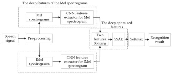
Figure 1.
Recognition network. The first channel extracts optimized features from the Mel spectrogram to highlight the low-frequency information, and the other channel extracts optimized features from the IMel spectrogram to highlight high-frequency information.
- (1)
- Preprocessing, which mainly includes endpoint detection, framing, and windowing, is performed.
- (2)
- The Mel spectrogram and IMel spectrogram, which are complementary, are generated.
- (3)
- The CNN-SSAE deep optimized features from the Mel spectrograms and IMel spectrograms are extracted and spliced.
- (4)
- The spliced features are sent to the softmax layer for identification.
4. IMel Spectrogram
This section describes the IMel spectrogram and its application to SER. First, the generation process and basic theory of the IMel spectrogram are introduced. Second, the performance of the IMel spectrogram is analyzed and compared with that of the Mel spectrogram.
4.1. Generation of the Mel Spectrogram
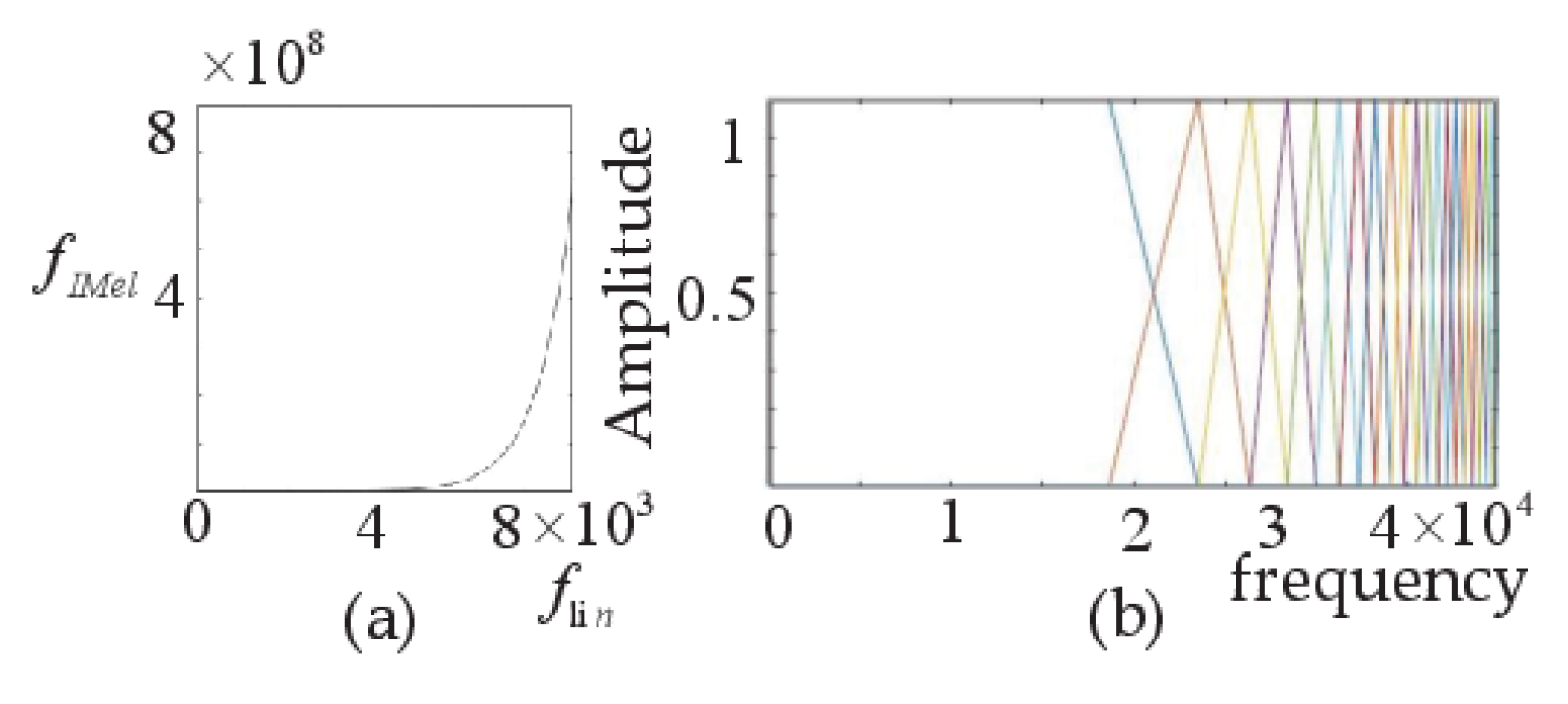
The commonly used Mel spectrogram contains the features of human auditory perception. It is based on the Mel frequency domain, in which linear frequencies are mapped to the Mel frequency. The equation below shows the relation:
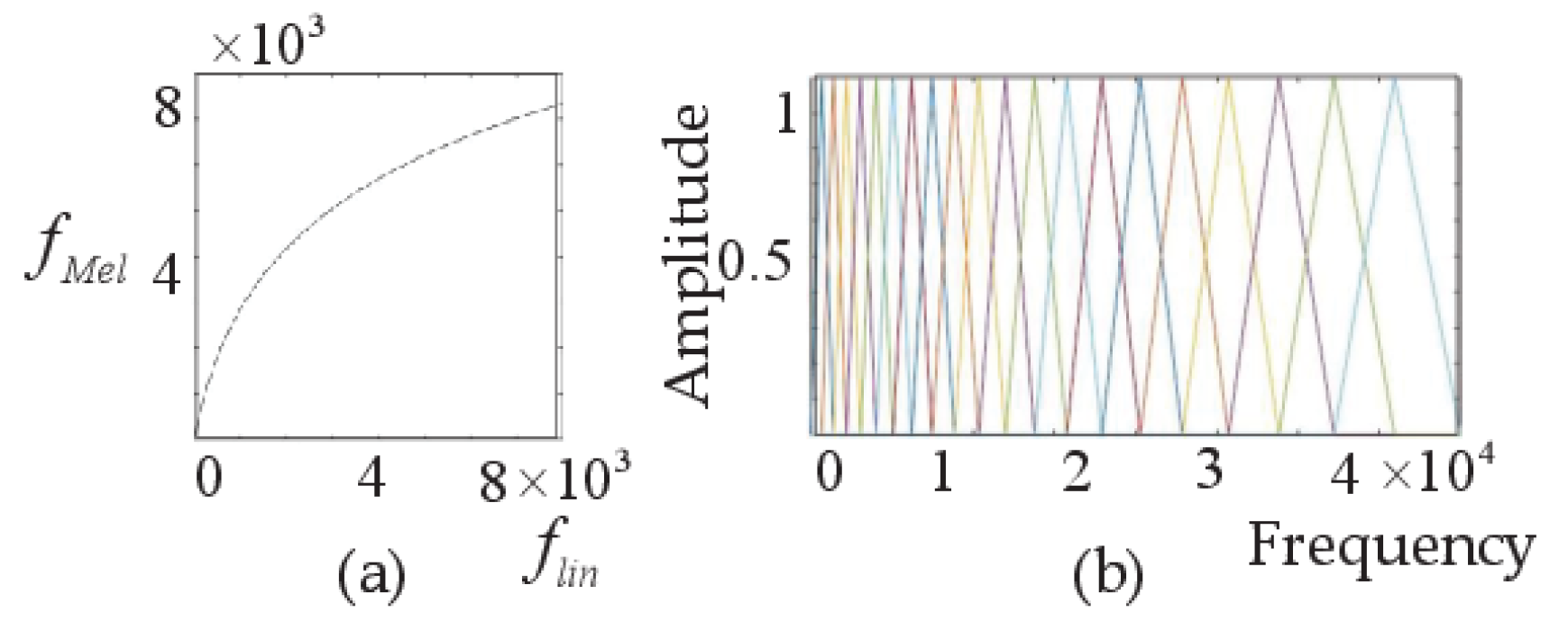
where is the frequency, expressed on a linear scale, and the unit is Hz; is the frequency on the Mel scale, and the unit is Mel. In Figure 2a, and are logarithms, and the resulting Mel filter banks are shown in Figure 2b. The resolution at the low frequency is higher than that at the high frequency, which is consistent with the characteristics of human hearing perception, and the Mel spectrogram based on the Mel filter banks has the same property. Therefore, the Mel spectrogram has been widely used and has achieved good results in the field of speech recognition. However, when applied to SER, it has certain limitations.
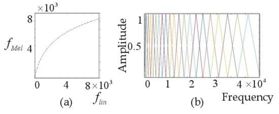
Figure 2.
(a) The relationship between flin and fMel. (b) Mel filter banks.
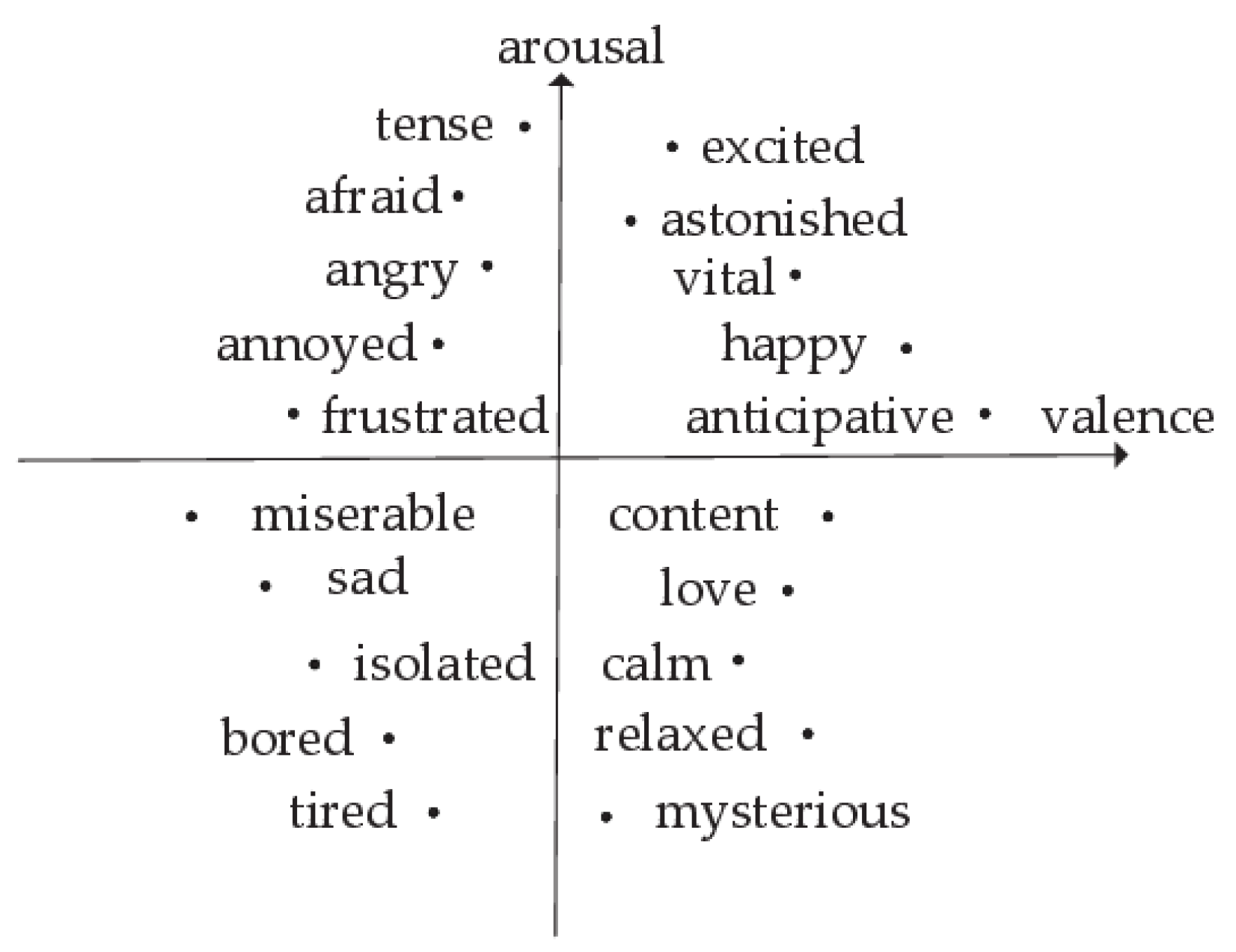
Figure 3 shows Russell’s two-dimensional expression of emotional space [53]. The abscissa is valence and the ordinate is arousal. Arousal indicates the intensity of emotions: a higher numerical value corresponds to a higher degree of emotional stimulation. The speech signals for high-aroused emotions, such as happiness and anger, include more quasi-periodic and low-frequency parts. The speech signals for Low-arousal emotions, such as sadness and tiredness, include more nonperiodic high-frequency parts and tail parts. The Mel spectrogram has a high resolution in the low-frequency part and is therefore suitable for high-arousal emotions. However, for some emotions with low arousal, more attention should be given to the high-frequency parts to achieve better SER. Therefore, in this paper, the IMel frequency domain is proposed and the IMel spectrogram, which is complementary to the Mel spectrogram and is generated by IMel filter banks, is obtained.

Figure 3.
Russell’s two-dimensional emotion spatial representation.
4.2. Generation of the IMel Spectrogram
The IMel spectrogram is generated by using an improved IMel filter bank, and the transformation relation is as follows:
is expressed in the IMel frequency domain, which is opposite to the Mel frequency domain. Figure 4a shows the exponential relationship between and in the IMel frequency domain. As shown in Figure 4b, the high-frequency part of the IMel filter banks has a narrow bandwidth and high resolution, thus enhancing the influence of high-frequency signals. Therefore, the IMel spectrograms generated using the IMel filter banks have the same characteristics.
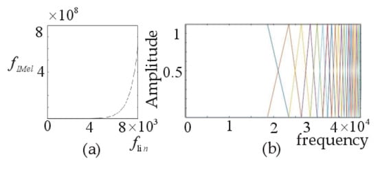
Figure 4.
(a) The relationship between and . (b) The IMel filter banks.
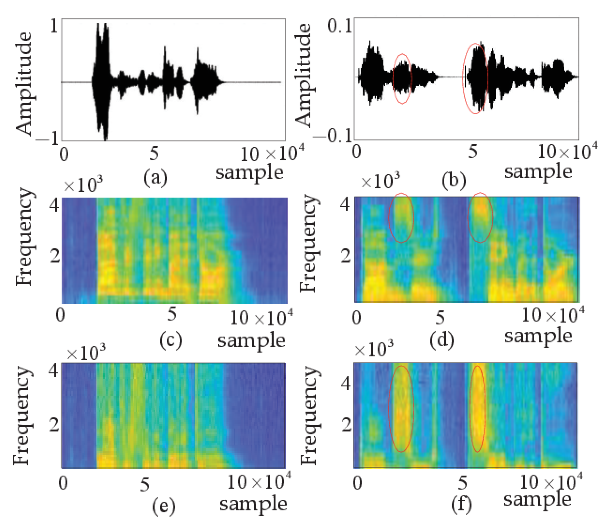
Figure 5a,b show the same person saying the same sentence “The dog is sitting by the door” with different emotions. In Figure 5a, anger is intense and quasi-periodic, with higher energy and more low-frequency parts. The speech in Figure 5a has the Mel spectrogram shown in Figure 5c, with clear stripes, highlighting the emotional information of the high-arousal signal. In Figure 5b, the speech is sad, weak, and low in energy, the range of the ordinate is [−0.1,0.1], which is ten times smaller than the range of angry speech. The unvoiced segment “S” in Figure 5b, marked by the ellipse, is the key point of detection. The Mel spectrogram in Figure 5d and the IMel spectrogram in Figure 5f corresponding to “S” are displayed in the ellipses. The IMel spectrogram amplifies the role of the high-frequency part and highlights the emotional information of the low-arousal signal. This paper combines the Mel spectrogram highlighting the low-frequency part with the IMel spectrogram highlighting the high-frequency part to apply their complementary effects to SER.
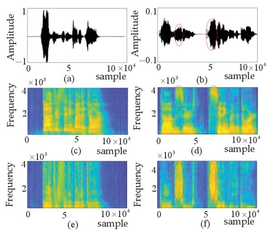
Figure 5.
(a) Speech signal of anger. (b) Speech signal of sad. (c) Mel spectrogram of anger. (d) Mel.spectrogram of sad. (e) IMel spectrogram of anger. (f) IMel spectrogram of sad.
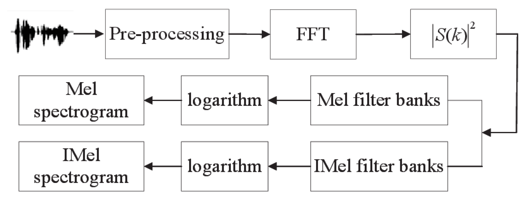
As shown in Figure 6, the speech signal is preprocessed, and then the energy obtained after a fast Fourier transform (FFT) is calculated. After passing through the Mel filter banks and the IMel filter banks separately, the logarithm is calculated, and finally the Mel spectrogram and the IMel spectrogram are obtained. The steps performed to generate the IMel spectrogram are as follows:
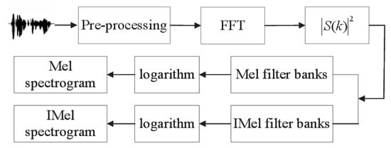
Figure 6.
The generation of Mel spectrogram and IMel spectrogram.
- (1)
- The speech signal is framed, where represents each frame and denotes the number of frames.
- (2)
- Windows are added, where the window function is a Hamming window and is the window length.
- (3)
- Each frame of the signal is transformed by FFT, , and the energy is obtained. is the number of points of the FFT.
- (4)
- and are converted from a linear scale to the IMel scale and are expressed as and :where and are the lowest frequency and the highest frequency of the filter frequency respectively.
- (5)
- The center frequency of each filter in the filter banks is Calculated:
- (6)
- The calculated center frequency of each filter is converted from the IMel scale to a linear scale:
- (7)
- The calculated center frequency on the linear scale is rounded to the nearest point of the FFT:
- (8)
- Where represents the transfer function of the IMel filter bank, the output is computed and the logarithm is calculated as , where is the number of filters, and the sample of each filter is . Finally, groups of are arranged vertically to form the IMel spectrogram of each frame, which is represented as .
- (9)
- The features of all frames are combined horizontally, and the IMel spectrogram is obtained.
5. CNN-SSAE Neural Network
As shown in Figure 1, the CNN-SSAE neural network proposed in this paper consists of a CNN and an SSAE. First, the spectrogram is taken as input, and the deep features are obtained by the CNN, Second, the deep optimized features are obtained by SSAE dimension reduction. Finally, the recognition results are classified through the softmax layer.
5.1. Convolutional Neural Network
The network structure of the CNN is shown in Figure 7 and the parameters of it are presented in Table 1. The CNN can transform the two-dimensional spectrogram into one-dimensional deep features to capture the emotional information of the speech. The characteristics of the CNN proposed in this paper are as follows: (1) After adding the batch normalization (BN) layer to the convolutional layers Con1, Con2, Con3 and Con4, the structure of the whole network is regularized to prevent overfitting, allow a higher learning rate, greatly improve the training efficiency, and solve the vanishing gradient problem. (2) The Global Average Pooling (GAP) layer is used instead of the fully connected layer. In the fully connected layer, a sub-region of each feature subgraph is set for averaging, the sub-regions are slid, and finally, all the average values are connected in series. In contrast, using GAP, each feature subgraph obtains an average value; this increases the emotional information somewhat, reduces the number of parameters, realizes model compression, and improves efficiency.
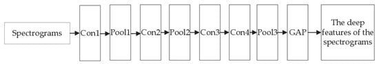
Figure 7.
The structure of the CNN.

Table 1.
CNN network architecture and parameter.
The deep features of the spectrogram obtained by the CNN may be redundant. Therefore, an SSAE is adopted to further optimize the deep features, reduce the number of dimensions, and improve the recognition rate.
5.2. Stacked Sparse Autoencoder
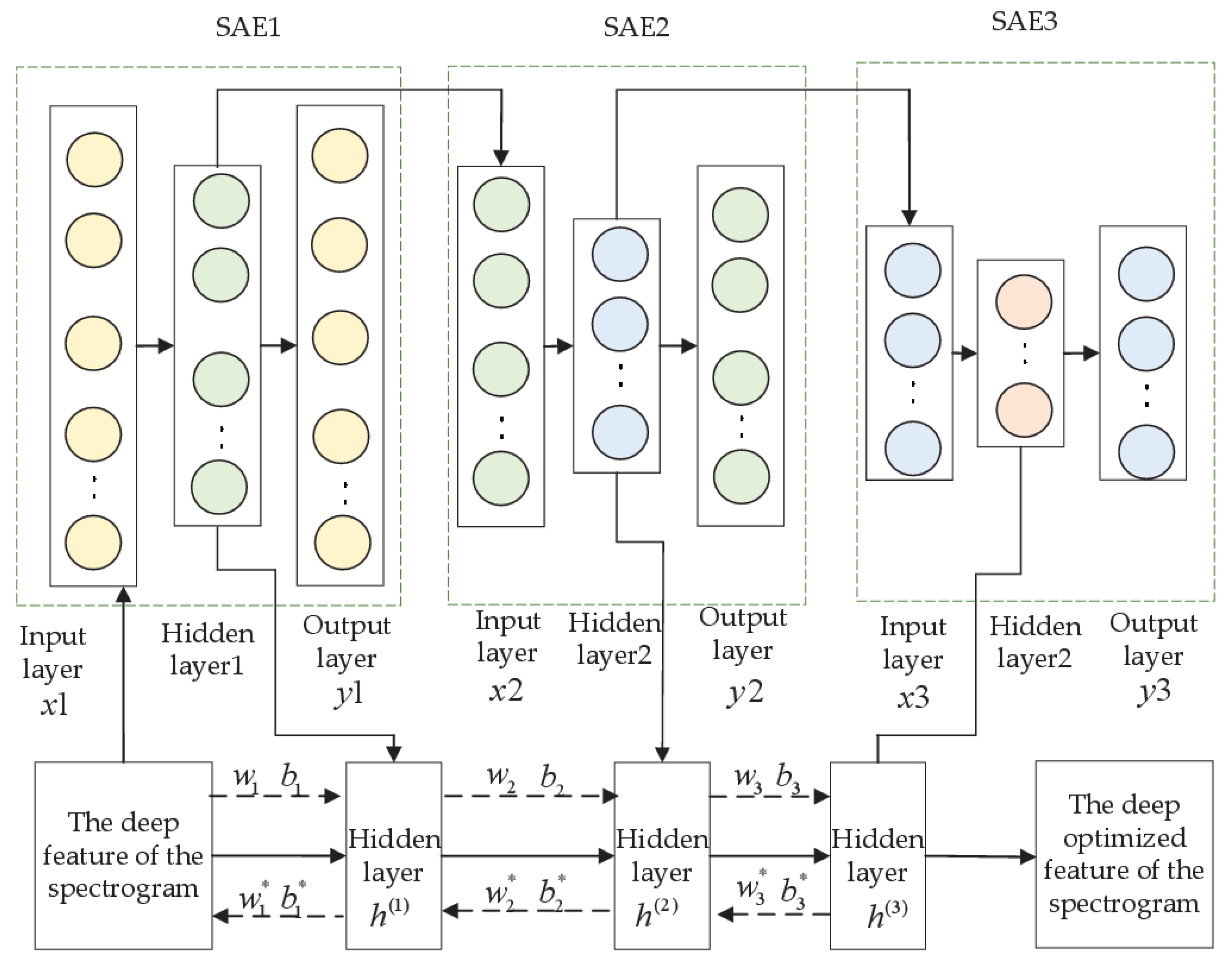
Multiple SAEs are stacked together to form an SSAE. It is suitable for the fusion and compression of information in input data and can extract necessary features. The SAE is usually used for data compression and fusion. The name refers to the sparse restrictions that are added to each hidden layer. The previous layer contains more hidden cells than the latter layer, and the hidden features learned in the latter layer are more abstract. This structure is similar to the working state of the human brain.
The SAE1 shown in Figure 8 is composed of an input layer, a hidden layer and an a output layer. The input data x1 are mapped to a hidden laye1; this is called the encoding process. The hidden layer1 is remapped to the reconstructed data y1; this is called the decoding process. This process should minimize the error function E from 1 to y1:
where denotes the number of samples, denotes the number of hidden layers, denotes the target value of the average activation degree, and denotes the average activation degree of the j-th layer.
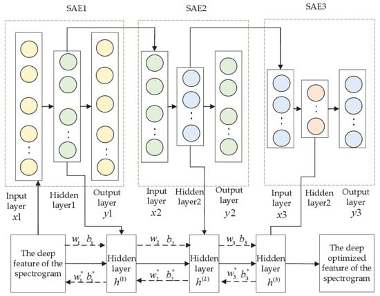
Figure 8.
The structure of the SSAE.
means distance (Kullback-Leibler divergence):
When training the network, the parameters should be constantly adjusted to minimum . A value of closer to 0 corresponds to a smaller average activation degree of the middle layer . In addition, it is necessary to constantly adjust the connection weight and bias to minimum the error function .
In the SSAE pre-training show in Figure 8, the weights and biases of each layer are and , the adjusted parameters are and , and the weights and biases after fine-tuning are and . SSAE is formed by stacking multiple layers. First, the 128-dimensional deep features of the spectrogram are as input layer of , whose hidden layer1 output is the 118-dimensional vector , where . Second, hidden layer1 is regarded as the input of , whose hidden layer2 output is the 108-dimensional vector , . Third, hidden layer2 is regarded as the input of , whose hidden layer output is the 98-dimensional vector , where . Finally, the deep optimized features are fed into the softmax layer for recognition.
6. Experiment
6.1. Experimental Datasets
To verify the effectiveness of our proposed spectrogram and dual-channel complementary model, we tested it on three widely used datasets: the Berlin dataset of German emotional speech (EMO-DB) [54], the Surrey Audio-Visual Expressed Emotion dataset (SAVEE) [55], and the Ryerson audiovisual dataset of emotional speech and song (RAVDESS) [56].
The EMO-DB database was created by researchers at the University of Berlin and is an emotional database in Germany. This database contains 535 utterances produced by 10 professional actors, including 5 males and 5 females), who produced 49, 58, 43, 38, 55, 35, 61, 69, 56, and 71 utterances respectively. These data are made up of seven different emotions: happiness, neutral, anger, boredom, disgust, sadness, and fear. The Sampling rate is 48 kHz (compressed to 16 kHz), and 16-bit quantization is adopted. It belongs to acted, and discrete type, access type is open, and modalities is audio.
The SAVEE database records the data of four native English-speaking males (DC, JE, JK, KL), graduate students and researchers from Surrey University, aged from 27 to 31. It contains a total of 480 utterances, each of which produces 120 utterances. The average length of each utterance is 4 s with a sampling rate of 44.1 kHz. This database consists of seven different emotions: happiness, sadness, anger, disgust, fear, neutral and surprise. It belongs to acted, and discrete type, access type is free, and modalities is audio/visual.
The RAVDESS database is an English emotional dataset, which consists of 1440 utterances produced by 24 actors, including 12 males and 12 females, who expressed eight different emotions: happiness, sadness, surprise, anger, calmness, disgust, fearfulness, and neutral. The database is widely used for emotional song and speech recognition, with a sampling rate of 48 kHz. It belongs to evoked and discrete types; access type is free and modalities are audio/visual.
In the above databases, emotion is expressed in different languages and cultures; for example, pronunciation characteristics of German and English differ; however, they have some common characteristics. Low-arousal emotions, such as sadness and disgust, have low energy and the speed of speech is generally slow. High-arousal emotions, such as happiness and anger, have high energy and the emotions are expressed strongly. For all datasets, the Mel spectrogram and IMel spectrogram are always complimentary.
6.2. Experimental Features
To verify that the Mel spectrograms and the IMel spectrograms are complementarity and to assess the effectiveness of the CNN-SSAE, six experimental features were designed.
- (1)
- Mel: The deep features of the Mel spectrogram were extracted by the CNN and sent to an SVM for recognition.
- (2)
- IMel: The deep features of the IMel spectrogram were extracted by the CNN and sent to an SVM for recognition.
- (3)
- Mel + IMel: The Mel deep features and IMel deep features were combined, and then send to an SVM for recognition.
- (4)
- MelSSAE: The Mel deep features were optimized and identified by the SSAE.
- (5)
- IMelSSAE: The IMel deep features were optimized and recognized by the SSAE.
- (6)
- (Mel + IMel) SSAE: The Mel deep features and IMel deep features were combined and then optimized and identified by the SSAE.
6.3. Parameter Settings
We chose the Hamming window to have a length of 25 ms and a shift of 10 ms and set the length of the FFT to 512. In the CNN-SSAE models, the batch size, learning rate of RMSProp, and dropout rate were set to 32, 0.001, and 0.1–0.2, respectively. To ensure the comprehensiveness of the experiment, fivefold cross-validation was adopted and the average value of five test results was taken to ensure the correctness of the experimental results.
6.4. Experimental Scenarios
To ensure that the experiment was comprehensive, we employed three experimental scenarios to analyze the results: speaker independent (SI), speaker-dependent (SD), and gender-dependent (GD) [57,58].
- (1)
- SD: The samples were randomly divided into two groups: the training set, containing 80%, and the test set, containing the remaining 20%.
- (2)
- SI: The samples were divided into two groups according to the subjects. The test set was composed of all the samples spoken by one subject, and the training set contained samples spoken by the remaining subjects.
- (3)
- GD: GD consists of two scenarios, GD-male and GD-female, according to gender. In the GD-male scenario, the samples were divided into two groups, with male data as the training set and female data as the test set. Conversely, in the GD-female scenario, female data were used as the training set, and male data were used as the test set.
6.5. Evaluation Indexes
Two evaluation indexes are used to measure the SER performance in this paper. The unweighted accuracy (UA) is the average value of recall for each class, and the weighted accuracy (WA) is the number of samples correctly classified divided by the total number of samples.
where the number of emotional categories is represented as , and the actual number of samples with this emotion is expressed as , is the number of samples correctly classified for emotion category .
6.6. Experimental Results and Analysis
6.6.1. Analysis of the IMel Spectrogram
(1) Factors influencing the spectrogram
How to get the most suitable spectrogram is the implementation challenge, because in the process of spectrogram implementation, the FFT length is 256, the window length is 256, the window shift is 128, and many other parameters have an impact on the results, such as the number M of filters and the frequency range R.
The number M of filters in the filter bank has an important influence on the display of the spectrogram. Figure 9a shows the filter banks with 20 filters, Figure 9b shows the Mel spectrogram corresponding to Figure 9a,c shows a filter bank with 40 filters, and Figure 9d shows the Mel spectrogram corresponding to Figure 9c. It can be observed that the spectrogram of Figure 9d is more detailed and obvious than that of Figure 9b, and is therefore more suitable for emotion detection.
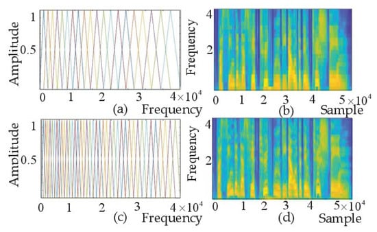
Figure 9.
(a) Mel filter banks M = 20. (b) Mel spectrogram M = 20. (c) Mel filter banks M = 40. (d) Mel.spectrogram M = 40.
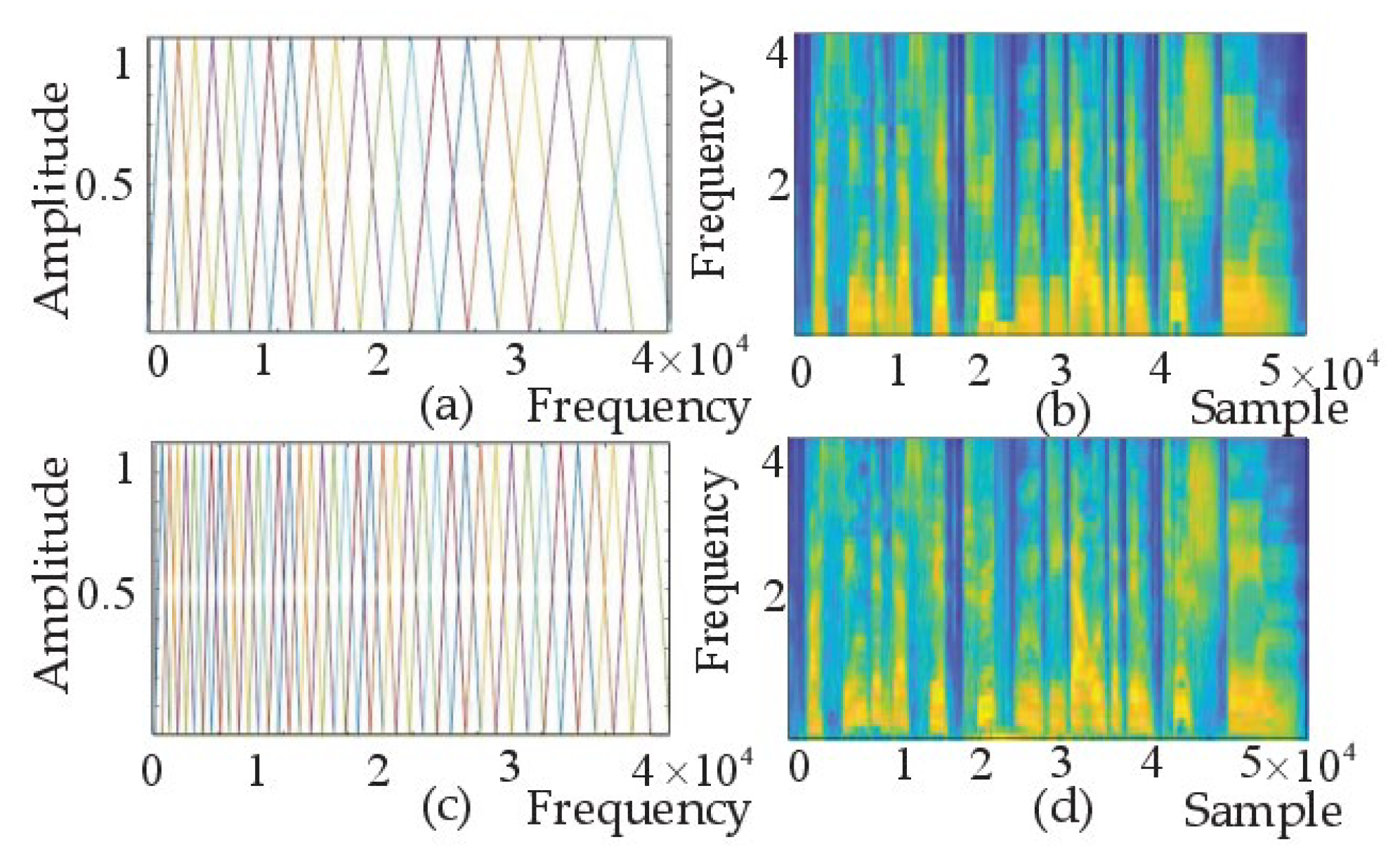
The vertical axis of the spectrogram indicates frequency and the horizontal axis indicates time. In this paper, represents the frequency range of the spectrogram and represents the maximum frequency. Both and have an important impact on recognition. According to the Nyquist principle, the maximum frequency is equal to half of the sampling frequency . For example, the sampling frequency of the SAVEE dataset is 44,200 Hz and the maximum frequency is 22,100 Hz. As shown in Figure 10a,c, the frequency ranges of the Mel filter banks and IMel filter banks are 0–4000 Hz, and Figure 10b,d show the corresponding Mel spectrogram and IMel spectrogram. In Figure 10e,g, the frequency ranges of the Mel filter and IMel filter are both 0–8000 Hz, and Figure 10f,h show the corresponding Mel spectrogram and IMel spectrogram. In Figure 10i,k, the frequency ranges of the Mel filter and IMel filter are both 0–21,000 Hz, and Figure 10j,l show the corresponding Mel spectrogram and IMel spectrogram. It can be observed that the low-frequency decomposition of the Mel spectrogram in Figure 10j is not sufficiently detailed, whereas the attention in Figure 10l is mostly in the invalid region. Therefore, the following work later section of this paper is to set the frequency range at 0–4000 Hz or 0–8000 Hz.
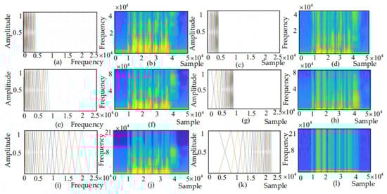
Figure 10.
(a) Mel filter banks R: 0–4000. (b) Mel spectrogram R: 0–4000. (c) IMel filter banks R:0–4000. (d) IMel spectrogram R: 0–4000. (e) Mel filter banks R: 0–8000. (f) Mel spectrogram R: 0–8000. (g) IMel filter banks R: 0–8000. (h) IMel spectrogram R: 0–8000. (i) Mel filter banks R: 0–21,000. (j) Mel spectrogram R: 0–21,000. (k) IMel filter banks R: 0–21,000. (l) IMel spectrogram R: 0–21,000.
(2) Complementarity analysis of Mel spectrogram and IMel spectrogram
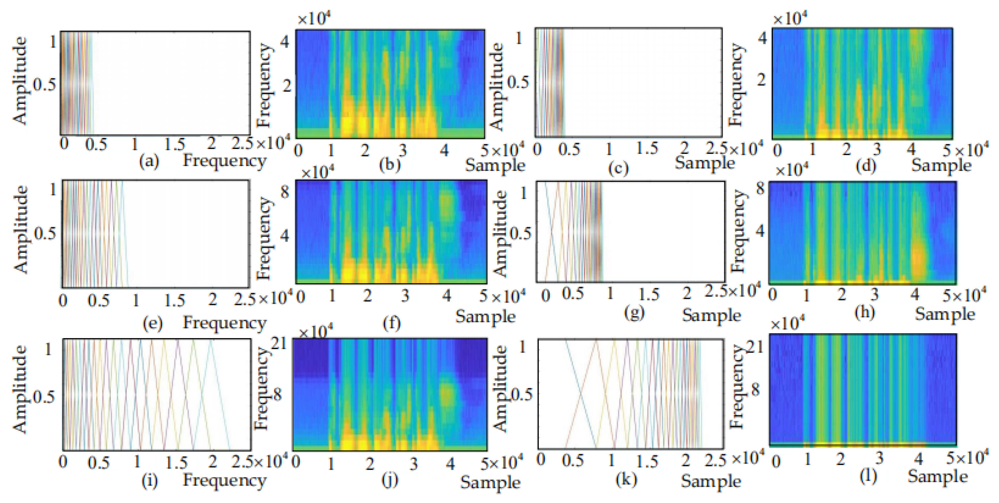
To prove that the Mel spectrogram and IMel spectrogram are complementary, the correlation analysis method is used in this paper. For two related variables, the correlation coefficient (whose value is between −1 and 1) indicates the degree of correlation. A greater absolute value of the correlation coefficient indicates more obvious emotional information and a brighter reflection in the image. As shown in Figure 11a–c, a correlation analysis of Mel deep features, IMel deep features, and Mel + IMel deep features of 480 sentences in the SAVEE database was conducted and expressed in the form of images. The abscissa and ordinate represent the 480 samples, The color of anger is bright in Figure 11a, dark in Figure 11b, and brighter in Figure 11c. The color of sadness is dark in Figure 11a, bright in Figure 11b, and brighter in Figure 11c. This shows that the Mel deep features and the IMel deep features are complementary, Moreover, the Mel + IMel deep features can maintain the advantage of each of them and can enhance the overall advantage, thereby playing a role in enhancing emotional information.
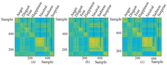
Figure 11.
(a) Correlation coefficient diagram of the Mel deep features. (b) Correlation coefficient diagram of the IMel deep features. (c) Correlation coefficient diagram of the Mel + IMel deep features.
6.6.2. Analysis of Recognition Accuracy
(1) Recognition results of each experimental scenarios
The sampling frequency of EMO-DB is 16,000 Hz, and that of SAVEE and RAVDESS is 44,200 Hz. Although the sampling frequencies are different, the frequency range of the speech signal is 200–3400 Hz. For all types of datasets, the energy is mainly concentrated in the range of 0–4000 Hz and there is some energy in the range of 4000–8000 Hz in some cases. From the above analysis, = 4000 Hz and = 8000 Hz were compared, In addition, to assess the influence of the number of filters M in the filter bank, M = 40, M = 60, and M = 80 were compared.
Table 2 shows that when = 8000 Hz, M = 60 and E = WA, the highest recognition rate of the EMO-DB database was 94.79 + 1.77%, that of the SAVEE database was 88.96 + 3.56%, and that of the RAVDESS database was 83.18 + 2.31%. This indicates that the frequency range of 0–8000 Hz reflects more comprehensive information. When the number M of filters was equal to 60, the decomposition of the spectrogram was more appropriate. Therefore, the following experiments for SI, GD and various types of emotion analysis were conducted with = 8000 Hz and M = 60.
Table 2.
SI Recognition Accuracy ± Standard Deviations (%).
Table 3.
SD Recognition Accuracy ± Standard Deviations (%).
Table 4.
GD-male Recognition Accuracy ± Standard Deviations (%).
Table 5.
GD-female Recognition Accuracy ± Standard Deviations (%).
- (1)
- The recognition accuracy of the Mel feature was higher than that of IMel, and the effect of using IMel alone was not as good as that of using Mel alone.
- (2)
- MelSSAE, IMelSSAE, and (Mel + IMel) achieved higher recognition accuracy than Mel, IMel, and Mel + IMel, respectively, thereby proving the effectiveness of the SSAE in dimension reduction.
- (3)
- The recognition accuracy of Mel + IMel was not necessarily higher than that of Mel or IMel, because directly splicing the two may contain redundancy and affect the recognition accuracy. However, after SSAE optimization, (Mel + IMel) SSAE improved the recognition accuracy of Mel, IMel, and Mel + IMel, thereby proving that Mel and IMel are complementary in deep features.
- (4)
- The standard deviation value is the average value that describes the distance that each recognition result deviates from the average. The values in the SI environment (Table 2) were less than the values in the SD and GD environments (Table 3, Table 4 and Table 5). This is because SI took all samples of one subject as the test set and other people’s samples as the training set, to reflect the similarity between individuals and groups. For example, GD-male took samples of all male subjects as the training set and samples of one female subject as the test set. To discover the similarity between different genders, there were large differences between the different genders, so the standard deviation of the recognition results was greater in the SI environment.
Although the experimental standards are different, the experimental results of SI, SD, and GD show the similar trends mentioned above; the results therefore prove the general applicability of this algorithm in this paper.
(2) Recognition accuracy of various emotions
Table 6 presents a comparison between the emotion recognition rate of the Mel feature and that of the IMel feature when = 8000 Hz and M = 60 in the three datasets. Figure 11 is a line chart corresponding to the recognition accuracy shown in Table 6. It can be observed that for high-arousal emotions, such as anger and happiness, the recognition accuracy of the Mel features was higher than that of the IMel features. For anger, the recognition accuracies of the Mel features were 94.83%, 80.17%, and 80.82%, respectively, and those of the IMel features were 88.71%, 71.67%, and 68.79%, respectively. These results indicate that the Mel spectrogram is more suitable for high-arousal emotions than the IMel spectrogram. For low-arousal emotions, such as sadness and disgust, the recognition accuracy of the IMel features was higher than that of the Mel features. For sadness, the recognition accuracies of the Mel features were 75.87%, 70.54%, and 66.87%, respectively, and those of the IMel features were 84.68%, 79.35%, and 70.96%, respectively. These results indicate that the IMel spectrogram is more suitable for low-arousal and high-frequency emotions than the Mel spectrogram.
Table 6.
Recognition Accuracy of Various Emotions (%).
(3) ROC curves
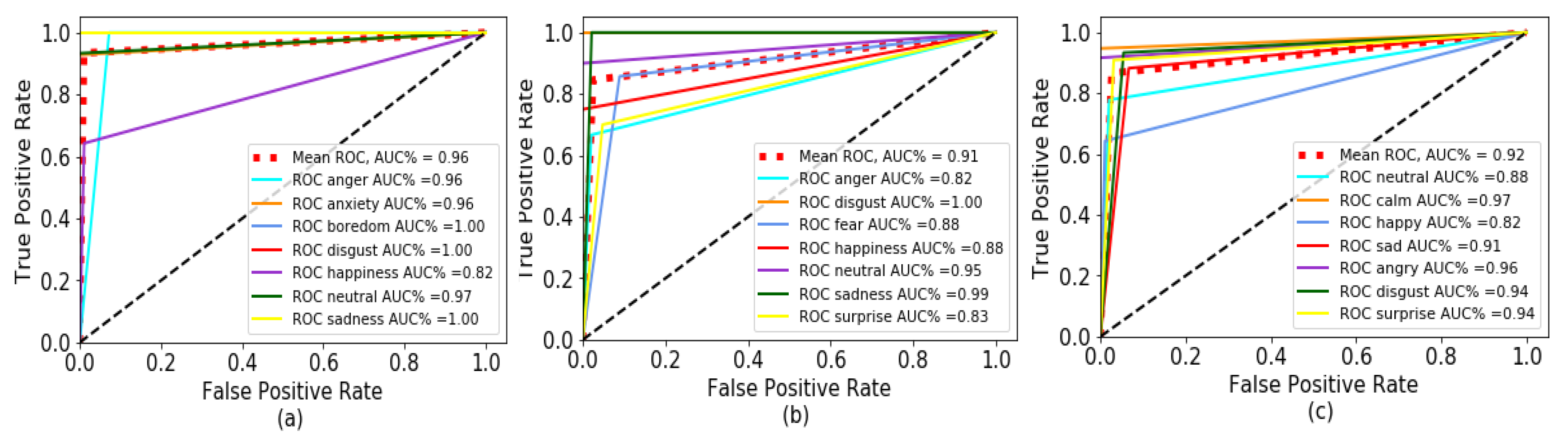
In Figure 12, the horizontal coordinate is the false Positive Rate, and the vertical coordinate is the ture positive Rate. AUC refers to the area under the ROC curve. Figure 12a presents the ROC curves of the system for ‘anger’, ‘anxiety’, ‘boredom’, ’disgust’, ‘happiness’, ‘neutral’, ‘sadness’ obtained by our proposed approach to the DBM-DB dataset, the red dashed line is the mean ROC value of each emotion. As can be seen from the figure, the system of this paper has good performance.
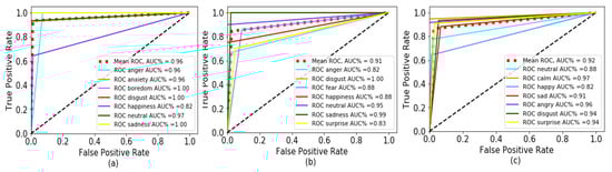
Figure 12.
(a) ROC curve of the system for EMO-DB. (b) ROC curve of the system for SAVEE. (c) ROC curve of the system for RAVDESS.
(4) The performance of the proposed system
Although the algorithm proposed in this paper has two CNN channels to extract the deep features, and doubles the number of parameters in terms of complexity, we can build two projects in Pycharm for Mel spectrogram and IMel spectrogram at the same time, and therefore there is no change in running time. The dimension of the single channel is 128, that of double channel is 256, and whether the input is 128 or 256 dimensions has little effect on the running time of SSAE.
(5) Comparison of various papers
Table 7 lists the results of the comparison between this paper and related papers published in recent years. The listed papers all use spectrograms to detect emotion. It can be observed that our method of combining the Mel spectrogram and IMel spectrogram is better than methods that use only a Mel spectrogram or a standard spectrogram.
Table 7.
Comparison of various papers in recent years.
7. Conclusions
In this paper, the frequency domain of IMel was proposed, and an IMel spectrogram that can highlight the high-frequency part was formed, which makes up for the shortage of Mel spectrograms that only highlight the low-frequency part. Then, a CNN-SSAE deep optimization network was presented. In this network, the two-dimensional spectrogram was sent to the CNN to obtain one-dimensional deep features, and then the internal redundant features were compressed and optimized by SSAE. The EMO-DB, SAVEE, and RAVDESS speech databases were used for experiments to verify the complementarity of the Mel spectrogram and IMel spectrogram and the effectiveness of CNN-SSAE in optimizing deep features. According to the current research situation, Although the proposed results obtained better recognition results, However, it also has limitations. The IMel filter is only the inverse process of the Mel filter, highlighting the high-frequency part. In the next step, wavelet algorithm, Hilbert–Huang transform, etc., can be used to highlight different frequency components of the layered signal; therefore, the next step will be to realize new spectrograms to obtain better recognition results. At present, the research tends to be multi-modal, combining the results of spectrogram with EEG features or kinematic features. In addition, the next step will be to extract better features through a deep optimized network, and obtain better recognition results.
Author Contributions
Conceptualization, J.L. and X.Z.; methodology, X.Z.; software, L.H.; validation, X.Z., F.L. and Y.S.; formal analysis, J.L.; investigation, S.D.; resources, X.Z. and S.D.; data curation, Y.S. and F.L.; writing—original draft preparation, J.L. and X.Z.; writing—review and editing, J.L., L.H. and S.D.; visualization, Y.S.; supervision, F.L.; project administration, J.L.; funding acquisition, L.H. All authors have read and agreed to the published version of the manuscript.
Funding
This work was supported in part by the National Nature Science Foundation of China under Grant 62271342, in part by “Project 1331” Quality Enhancement and Efficiency Construction Plan National First-class Major Construction Project of Electronic Science and Technology, in part by the National Natural Science Foundation of China Youth Science Foundation under Grant 12004275, in part by the Natural Science Foundation of Shanxi Province, China, under Grant 201901D111096, in part by Research Project Supported by Shanxi Scholarship Council of China HGKY2019025.
Institutional Review Board Statement
Not applicable.
Informed Consent Statement
Not applicable.
Conflicts of Interest
The authors declare no conflict of interest.
References
- Yildirim, S.; Kaya, Y.; Kili, F. A modified feature selection method based on metaheuristic algorithms for speech emotion recognition. Appl. Acoust. 2021, 173, 107721. [Google Scholar] [CrossRef]
- Fahad, M.S.; Ashish, R.; Jainath, Y.; Akshay, D. A survey of speech emotion recognition in natural environment science direct. Digit. Signal Process. 2021, 110, 102951. [Google Scholar] [CrossRef]
- Wang, S.H.; Phillips, P.; Dong, Z.C.; Zhang, Y.D. Intelligent facial emotion recognition based on stationary wavelet entropy and Jaya algorithm. Neurocomputing 2018, 272, 668–676. [Google Scholar] [CrossRef]
- Gunes, H.; Piccardi, M. Bi-modal emotion recognition from expressive face and body gestures. J. Netw. Comput. Appl. 2007, 30, 1334–1345. [Google Scholar] [CrossRef]
- Noroozi, F.; Corneanu, C.A.; Kaminska, D.; Sapinski, T.; Escalera, S.; Anbarjafari, G. Survey on emotional body gesture recognition. IEEE Trans. Affect. Comput. 2021, 12, 505–523. [Google Scholar] [CrossRef]
- Islam, M.R.; Moni, M.A.; Islam, M.M.; Rashed-Al-Mahfuz, M.; Islam, M.S.; Hasan, M.K.; Hossain, S.; Ahmad, M.; Uddin, S.; Azad, A.; et al. Emotion recognition from EEG signal focusing on deep learning and shallow learning techniques. IEEE Access 2021, 9, 94601–94624. [Google Scholar] [CrossRef]
- Abbaschian, B.J.; Sierra-Sosa, D.; Elmaghraby, A. Deep learning techniques for speech emotion recognition from databases to models. Sensors 2021, 21, 1249. [Google Scholar] [CrossRef] [PubMed]
- Zhang, H.; Huang, H.; Han, H. A novel heterogeneous parallel convolution bi-LSTM for speech emotion recognition. Appl. Sci. 2021, 11, 9897. [Google Scholar] [CrossRef]
- El Ayadi, M.; Kamel, M.S.; Karray, F. Survey on speech emotion recognition: Features, classification schemes, and databases. Pattern Recognit. 2011, 44, 572–587. [Google Scholar] [CrossRef]
- Akçay, M.B.; Oğuz, K. Speech emotion recognition: Emotional models, databases, features, preprocessing methods, supporting modalities, and classifiers. Speech Commun. 2020, 116, 56–76. [Google Scholar] [CrossRef]
- Cheng, L.; Zong, Y.; Zheng, W.; Li, Y.; Tang, C.; Schuller, B.W. Domain Invariant Feature Learning for Speaker-Independent Speech Emotion Recognition. IEEE/ACM Trans. Audio Speech Lang. Process. 2022, 30, 2217–2230. [Google Scholar]
- Ozer, I. Pseudo-colored rate map representation for speech emotion recognition. Biomed. Signal Process. Control 2021, 66, 102502. [Google Scholar] [CrossRef]
- Prasomphan, S. Detecting human emotion via speech recognition by using speech spectrogram. In Proceedings of the 2015 IEEE International Conference on Data Science and Advanced Analytics (DSAA), Paris, France, 19–21 October 2015; pp. 1–10. [Google Scholar]
- Jiang, P.; Fu, H.; Tao, H.; Lei, P.; Zhao, L. Parallelized convolutional recurrent neural network with spectral features for speech emotion recognition. IEEE Access 2019, 7, 90368–90377. [Google Scholar] [CrossRef]
- Farooq, M.; Hussain, F.; Baloch, N.K.; Raja, F.R.; Yu, H.; Zikria, Y.B. Impact of feature selection algorithm on speech emotion recognition using deep convolutional neural network. Sensors 2020, 20, 6008. [Google Scholar] [CrossRef]
- Khalil, R.A.; Jones, E.; Babar, M.I.; Jan, T.; Zafar, M.H.; Alhussain, T. Speech emotion recognition using deep learning techniques: A review. IEEE Access 2019, 7, 117327–117345. [Google Scholar] [CrossRef]
- Chen, L.F.; Su, W.J.; Feng, Y.; Wu, M.; Hirota, K. Two-layer fuzzy multiple random forest for speech emotion recognition in human-robot interaction. Inf. Sci. 2019, 509, 150–163. [Google Scholar] [CrossRef]
- Zhang, S.Q.; Zhang, S.L.; Huang, T.J.; Huang, T.J.; Gao, W. Speech Emotion Recognition Using Deep Convolutional Neural Network and Discriminant Temporal Pyramid Matching. IEEE Trans. Multimed. 2017, 20, 1576–1590. [Google Scholar] [CrossRef]
- Lieskovská, E.; Jakubec, M.; Jarina, R.; Chmulík, M. A review on speech emotion recognition using deep learning and attention mechanism. Electronics 2021, 10, 1163. [Google Scholar] [CrossRef]
- Sugan, N.; Srinivas, N.S.S.; Kumar, L.S.; Nath, M.K.; Kanhe, A. Speech emotion recognition using cepstral features extracted with novel triangular filter banks based on bark and erb frequency scales. Biomed. Signal Process. Control 2020, 104, 102763. [Google Scholar]
- Zheng, C.S.; Tan, Z.H.; Peng, R.H.; Li, X.D. Guided spectrogram filtering for speech dereverberation. Appl. Acoust. 2018, 134, 154–159. [Google Scholar] [CrossRef]
- Liu, Z.T.; Xie, Q.; Wu, M.; Cao, W.H.; Mei, Y.; Mao, J.W. Speech emotion recognition based on formant characteristics feature extraction and phoneme type convergence. Inf. Sci. 2021, 563, 309–325. [Google Scholar] [CrossRef]
- Satt, A.; Rozenberg, S.; Hoory, R. Efficient Emotion Recognition from Speech Using Deep Learning on Spectrograms. In Proceedings of the Annual Conference of the International Speech Communication Association, INTERSPEECH, Stockholm, Sweden, 20–24 August 2017. [Google Scholar]
- Yao, Z.W.; Wang, Z.H.; Liu, W.H.; Liu, Y.Q. Speech emotion recognition using fusion of three multi-task learning-based classifiers: HSF-DNN, MS-CNN and LLD-RNN. Speech Commun. 2020, 120, 11–19. [Google Scholar] [CrossRef]
- Daneshfar, F.; Kabudian, S.J. Speech emotion recognition using discriminative dimension reduction by employing a modified quantumbehaved particle swarm optimization algorithm. Multimed. Tools Appl. 2020, 79, 1261–1289. [Google Scholar] [CrossRef]
- Yuan, J.; Chen, L.; Fan, T.; Jia, J. Dimension reduction of speech emotion feature based on weighted linear discriminate analysis. Image Process. Pattern Recognit. 2015, 8, 299–308. [Google Scholar]
- Sahu, S.; Gupta, R.; Sivaraman, G.; AbdAlmageed, W.; Espy-Wilson, C. Adversarial auto-encoders for speech based emotion recognition. arXiv 2018, arXiv:1806.02146. [Google Scholar]
- Mao, Q.; Dong, M.; Huang, Z.; Zhan, Y. Learning salient features for speech emotion recognition using convolutional neural networks. IEEE Trans. Multimedia. 2014, 16, 2203–2213. [Google Scholar] [CrossRef]
- Ancilin, J.; Milton, A. Improved speech emotion recognition with Mel frequency magnitude coefficient. Appl. Acoust. 2021, 179, 108046. [Google Scholar] [CrossRef]
- Nwe, T.L.; Foo, S.W.; Silva, L.C.D. Speech emotion recognition using hidden markov models. Speech Commun. 2003, 41, 603–623. [Google Scholar] [CrossRef]
- Diana, T.B.; Meshia, C.O.; Wang, F.N.; Jiang, D.M.; Verhelst, W.; Sahli, H. Hierarchical sparse coding framework for speech emotion recognition. Speech Commun. 2018, 99, 80–89. [Google Scholar]
- Kerkeni, L.; Serrestou, Y.; Raoof, K.; Mbarki, M.; Mahjoub, M.A.; Cleder, C. Automatic speech emotion recognition using an optimal combination of features based on EMD-TKEO. Speech Commun. 2019, 114, 22–35. [Google Scholar] [CrossRef]
- Sun, Y.; Zhang, X.Y. Characteristics of human auditory model based on compensation of glottal features in speech emotion recognition. Future Gener. Comput. Syst. 2018, 81, 291–296. [Google Scholar]
- Yang, B.; Lugger, M. Emotion recognition from speech signals using new harmony features. Signal Process. 2010, 99, 1415–1423. [Google Scholar] [CrossRef]
- Sun, Y.X.; Wen, G.H.; Wang, J.B. Weighted spectral features based on local Hu moments for speech emotion recognition. Biomed. Signal Process. Control 2015, 18, 80–90. [Google Scholar] [CrossRef]
- Badshah, A.; Rahim, N.; Ullah, N.; Ahmad, J. Deep features based speech emotion recognition for smart affective services. Multimed. Tools Appl. 2019, 78, 5571–5589. [Google Scholar] [CrossRef]
- Anvarjon, T.; Mustaqeem; Kwon, S. Deep-Net: A Lightweight CNN-Based Speech Emotion Recognition System Using Deep Frequency Features. Sensors 2020, 20, 5212. [Google Scholar] [CrossRef]
- Minji, S.; Myungho, K. Fusing Visual Attention CNN and Bag of Visual Words for Cross-Corpus Speech Emotion Recognition. Sensors 2020, 20, 5559. [Google Scholar]
- Chen, M.Y.; He, X.J.; Yang, J.; Zhang, H. 3-D Convolutional Recurrent Neural Networks with Attention Model for Speech Emotion Recognition. IEEE Signal Process. Lett. 2018, 25, 1440–1444. [Google Scholar] [CrossRef]
- Liu, D.; Shen, T.S.; Luo, Z.L.; Zhao, D.X.; Guo, S.J. Underwater target recognition using convolutional recurrent neural networks with 3-D Mel-spectrogram and data augmentation. Appl. Acoust. 2021, 178, 107989. [Google Scholar] [CrossRef]
- Hajarolasvadi, N.; Demirel, H. 3D CNN-Based Speech Emotion Recognition Using K-Means Clustering and Spectrograms. Entropy 2019, 21, 479. [Google Scholar] [CrossRef]
- Zhang, X.; Song, P.; Cha, C. Time frequency atomic auditory attention model for cross database speech emotion recognition. J. Southeast Univ. 2016, 4, 11–16. [Google Scholar]
- Yu, Y.; Kim, Y. Attention-LSTM-Attention Model for Speech Emotion Recognition and Analysis of IEMOCAP Database. Electronics 2020, 9, 713. [Google Scholar] [CrossRef]
- Eyben, F.; Wöllmer, M.; Schuller, B. Opensmile: The munich versatile and fast open-source audio feature extractor. In Proceedings of the 18th ACM international conference on Multimedia, Firenze, Italy, 25–29 October 2010; pp. 1459–1462. [Google Scholar]
- Ozseven, T. Investigation of the effect of spectrogram images and different texture analysis methods on speech emotion recognition. Appl. Acoust. 2018, 142, 70–77. [Google Scholar] [CrossRef]
- Liu, Z.T.; Xie, Q.; Wu, M.; Cao, W.H.; Mei, Y.; Mao, J.W. Speech emotion recognition based on an improved brain emotion learning model. Neurocomputing 2018, 309, 145–156. [Google Scholar] [CrossRef]
- Yogesh, C.K.; Hariharanb, M.; Ngadirana, R.; Adomb, A.H.; Yaacobc, S.; Berkai, C.; Polat, K. A new hybrid pso assisted biogeography-based optimization for emotion and stress recognition from speech signal. Expert Syst. Appl. 2017, 69, 149–158. [Google Scholar]
- Daneshfar, F.; Kabudian, S.J.; Neekabadi, A. Speech emotion recognition using hybrid spectral-prosodic features of speech signal/glottal waveform, metaheuristic-based dimensionality reduction, and Gaussian elliptical basis function network classifier. Appl. Acoust. 2020, 166, 107360. [Google Scholar] [CrossRef]
- Xu, J.; Xiang, L.; Liu, Q.S.; Gilmore, H.; Wu, J.Z.; Tang, J.H.; Madabhushi, A. Stacked Sparse Autoencoder (SSAE) for Nuclei Detection on Breast Cancer Histopathology Images. IEEE Trans. Med. Imaging 2015, 35, 119–130. [Google Scholar] [CrossRef]
- Tang, Q.L.; Fang, Q.; Xia, X.F.; Yang, J.R. Breast pathology image cell identification based on stacked sparse autoencoder and holistically-nested structure. J. South-Cent. Univ. Natl. Nat. Sci. Ed. 2019, 3, 397–403. [Google Scholar]
- Mufidah, R.; Wasito, I.; Hanifah, N.; Faturrahman, M.; Ghaisani, F.D. Automatic nucleus detection of pap smear images using stacked sparse autoencoder (ssae). In Proceedings of the International Conference on Algorithms Computing and Systems, Jeju Island Republic of Korea, 10–13 August 2017; pp. 9–13. [Google Scholar]
- Li, S.Q.; Jiang, H.Y.; Bai, J.; Liu, Y.; Yao, Y.D. Stacked sparse autoencoder and case-based postprocessing method for nucleus detection. Neurocomputing 2019, 24, 494–508. [Google Scholar] [CrossRef]
- Quan, X.L.; Zeng, Z.G.; Jiang, J.H.; Zhang, Y.Q.; LV, B.L.; Wu, D.R. Physiological signals based affective computing: A systematic review. Acta Autom. Sin. 2021, 8, 1769–1784. [Google Scholar]
- Burkhardt, F.; Paeschke, A.; Rolfes, M.; Sendlmeier, W.F. A database of german emotional speech; INTERSPEECH 2005—Eurospeech. In Proceedings of the 9th European Conference on Speech Communication and Technology, Lisbon, Portugal, 4–8 September 2005. [Google Scholar]
- Jackson, P.J.B.; Haq, S.U. Surrey Audio-Visual Expressed Emotion (Savee) Database; University of Surrey: Guildford, UK, 2014. [Google Scholar]
- Livingstone, S.R.; Russo, F.A. The ryerson audio-visual database of emotional speech and song (ravdess): A dynamic, multimodal set of facial and vocal expressions in north American English. PLoS ONE 2018, 13, e0196391. [Google Scholar] [CrossRef]
- Yogesh, C.K.; Hariharan, M.; Ngadiran, R.; Adom, A.H.; Yaacob, S.; Polat, K. Hybrid bbo pso and higher order spectral features for emotion and stress recognition from natural speech. Appl. Soft Comput. 2017, 56, 217–232. [Google Scholar]
- Wang, K.X.; Su, G.X.; Liu, L.; Wang, S. Wavelet packet analysis for speaker-independent emotion recognition. Neurocomputing 2020, 398, 257–264. [Google Scholar] [CrossRef]


Publisher’s Note: MDPI stays neutral with regard to jurisdictional claims in published maps and institutional affiliations. |
© 2022 by the authors. Licensee MDPI, Basel, Switzerland. This article is an open access article distributed under the terms and conditions of the Creative Commons Attribution (CC BY) license (https://creativecommons.org/licenses/by/4.0/).