Article

Development and Comparison of Ten Differential-Evolution and Particle Swarm-Optimization Based Algorithms for Discount-Guaranteed Ridesharing Systems

Department of Computer Science and Information Engineering, Chaoyang University of Technology, Taichung 413310, Taiwan
Appl. Sci. 2022, 12(19), 9544; https://doi.org/10.3390/app12199544
Submission received: 18 August 2022 / Revised: 14 September 2022 / Accepted: 19 September 2022 / Published: 23 September 2022

Abstract

:
Savings on transportation costs provide an important incentive for shared mobility models in smart cities. Therefore, the problem of maximizing cost savings has been extensively studied in the ridesharing literature. Most studies on ridesharing focus on the maximization of the overall savings on transportation costs. However, the maximization of the overall savings on transportation costs may satisfy users’ expectations for cost savings. For people to adopt ridesharing as a means to reduce costs, a minimal expected cost savings discount must be offered. There is obviously a gap between the existing studies and the real problems faced by service providers. This calls for the development of a study to formulate a ridesharing model that guarantees the satisfaction of a minimal expected cost savings discount. In this paper, we considered a discount-guaranteed ridesharing model that ensures the provision of a minimal expected cost savings discount to ridesharing participants to improve users’ satisfaction with the ridesharing service in terms of cost savings. The goal was to maximize the overall cost savings under certain capacity, spatial, and time constraints and the constraint that the discount offered to ridesharing participants could be no lower than the minimal expected cost savings discount. Due to the complexity of the optimization problem, we adopted two evolutionary computation approaches, differential evolution and particle swarm optimization, to develop ten algorithms for solving the problem. We illustrated the proposed method by an example. The results indicated that the proposed method could guarantee that the discount offered to ridesharing participants was greater than or equal to the minimal expected cost savings discount. We also conducted two series of experiments to assess the performance and efficiency of the different solution algorithms. We analyzed the results to provide suggestions for selecting the appropriate solution algorithm based on its performance and efficiency.

1. Introduction

Under the pressure of environmental protection and global warming, transportation service providers have evolved from providing dedicated rides to offering shared rides for travelers/customers in the sharing economy era. A variety of shared mobility transport models have appeared in the past decade. For transport policy makers and service providers, an important issue is formulating shared mobility transport models that are accepted by users in order to reduce energy consumption and the emission of greenhouse gases.
There are several factors influencing the acceptance of shared mobility transport models [1,2,3,4,5]. These include economic factors such as cost savings and non-economic factors such as safety and trust. As transportation costs constitute a large part of industry and daily-life expenses, savings on transportation costs provide an important incentive for shared mobility models in smart cities. In a ridesharing system, the ridesharing participants include drivers and passengers. If a driver travels alone without ridesharing, the travel cost will be paid by the driver. Similarly, a passenger traveling alone without ridesharing also has to pay the travel cost by him/herself. Suppose the itineraries of a driver and a set of passengers are spatially and temporarily similar: the driver may share the ride with the set of passengers. If the overall costs of the shared ride are less than the overall travel costs of the driver and the set of passengers, cost savings are achieved. Based on the above reasoning, most studies on ridesharing attempt to maximize the overall cost savings. Therefore, the problem of maximizing coast savings has been extensively studied in the ridesharing literature [6,7].
Most studies on ridesharing focus on the maximization of the overall savings on transportation costs. However, the maximization of the overall savings on transportation costs may not lead to the satisfaction of users’ expectation for cost savings. Ridesharing is attractive for drivers and passengers only if the portion of cost savings allocated to each of them is no lower than their expectations. In this study, to describe drivers’ and passengers’ expectations of cost savings, we used “minimal expected cost savings discount” to refer to the reduction in costs expected by drivers and passengers. If drivers’ and passengers’ minimal expected cost savings discounts are not met, ridesharing is not attractive. Therefore, ridesharing models must satisfy participants’ minimal expected cost savings discounts, as they are directly related to participants’ acceptance of and satisfaction with ridesharing. For people to adopt ridesharing as a means to reduce costs, a minimal expected cost savings discount must be offered. There is obviously a gap between the existing studies and the real problems faced by service providers. This calls for the development of a decision model to formulate a ridesharing system that meets users’ expectations for cost savings. In this paper, we introduce the concept of the minimal expected cost savings discount and formulate a discount-guaranteed ridesharing model that maximizes the overall cost savings under the constraint that the cost savings discount for users cannot be lower than the minimal expected cost savings discount.
As a ridesharing system typically consist of drivers, passengers, and a service provider, it can be modeled as a multi-agent system (MAS) [8,9]. In a MAS, an agent is a cooperative, autonomous, and intelligent entity working to achieve certain goals. MASs have been applied to a variety of complex problems. By representing drivers, passengers, and the service provider as agents, the MAS paradigm can be used to model a ridesharing system. In this paper, we adopted the MAS concept to model a ridesharing system. Our MAS included driver agents, passenger agents, and a service provider agent. The driver agents and passenger agents submit bids to the system, and the service provider agent must determine the winning bids. The operation of the MAS is very similar to auctions [10]. Modeling transportation systems with combinatorial auctions in a MAS was studied in [11]. The problem setting of ridesharing systems is more complex due to the presence of many transportation constraints on the side of both the driver agents and the passenger agents. Therefore, although the operation of a ridesharing system is similar to that of combinatorial double auctions in a MAS, the constraints on ridesharing systems are different to those on classic combinatorial double auctions. These differences pose a challenge for determining the winning bids for ridesharing systems. Applying combinatorial double auctions in a MAS to model ridesharing system has been studied in [12]. In this paper, we follow the double auction model of [12] and extend the additional constraints to incorporate the discount guarantee aspect of our ridesharing system. Due to exponential growth of the solution space and the number of solutions, finding a solution for classical combinatorial double auctions is already challenging from a computational point of view [13,14]. A general combinatorial double auction is known to be an NP-hard problem in terms of computational complexity [14]. The constraints related to the issue of the guaranteed discount introduced additional complexity and posed a new challenge. Due to the complexity of the optimization problem, we adopted two evolutionary computation approaches [15,16] to solve the problem. Ten algorithms were developed, and we illustrated the proposed method by an example. The results indicated that the proposed method could guarantee that the cost savings discount for users was no lower than the minimal expected cost savings discount. We compared the performance and efficiency of the ten algorithms proposed in this study by conducting two series of experiments and analyzing the results. Our findings provide insight into the selection of an appropriate algorithm to solve the discount-guaranteed ridesharing problem.
The contributions of this paper are threefold:
  • First, we propose a decision problem that offers a minimal cost savings discount for drivers and passengers. The ability to offer a minimal cost savings discount to users is essential for incentivizing participants to accept a ridesharing model. However, the existing literature and our previous paper only focused on the maximization of the overall savings or benefits. The issue of guaranteeing a minimal cost savings discount in ridesharing systems has not been addressed in the literature. Hence, the problem addressed and the decision model proposed in this paper are different from those discussed in our previous studies and the existing literature, in that we focus on the discount-guaranteed ridesharing problem.
  • Second, ten solution algorithms are proposed in this study to provide decision support tools for finding a set of users for whom the minimal cost savings discount can be guaranteed and the total cost savings achieved can be optimized.
  • Third, we compare the proposed algorithms by analyzing the results of several test cases to provide a guideline for selecting an appropriate solution algorithm.
The organization of the rest of this paper is as follows. A review of the ridesharing literature is provided in Section 2. Following the literature review, the details of the discount-guaranteed ridesharing problem are described and formulated in Section 3. Several approaches to solving the discount-guaranteed ridesharing problem are proposed in Section 4. The experiments carried out based on the proposed methods are reported in Section 5, which consists of two subsections: an example for the verification of the proposed solution method is illustrated in Section 5.1, and a comparison of the ten algorithms is performed in Section 5.2. In Section 6, we analyze and discuss the results. Finally, we draw our conclusions in Section 7.

2. Literature Review

Ridesharing is a shared mobility transport mode that enables travelers or drivers/passengers with similar itineraries to share rides and enjoy cost savings. In addition to cost savings, the potential benefits of reduced fuel consumption, vehicles numbers, air pollution, and traffic congestion have made ridesharing an attractive transport mode for pursuing sustainability. Studies have examined the factors affecting peoples’ intentions to use other types of information systems, such as distance learning systems [17]. The adoption of ridesharing systems is also influenced by several factors [18]. Due to the potential benefits of ridesharing, many studies have been conducted to assess the drivers, barriers, and determinants for ridesharing [2,3,4]. In [5], Mitropoulos et al. provide a literature review of ridesharing platforms, focusing on the user factors and barriers to ridesharing. Shared transportation has economic benefits for users, companies, and societies [19]. In particular, cost and convenience are two important factors affecting ridesharing [20]. The early work of [21] focused on studying the determinants of employee ridesharing. The authors indicated that a long commute tends to encourage ridesharing more than a short commute. This is primarily because a more extensive portion of the route is usually shared between commuters in a longer commute, leading to greater cost savings and hence encouraging ridesharing. Ridesharing is not limited to sharing rides using private cars. Recently, the ridesharing concept has also been applied to the planning of buses to improve their ridesharing success rate [22].
The importance and challenges of ridesharing problems have driven academic researchers and industry practitioners to study the diversified issues of ridesharing systems. Relevant studies on ridesharing can be found in several survey papers in the literature. Early studies on ridesharing can be found in [6,7]. Reference [1] provides discussions on the benefits and challenges of shared mobility services. Many issues related to ridesharing have been studied in the literature. These issues include cost savings, [23], the allocation of cost savings [24,25], social awareness [26], enjoyability [27], trust [28], empty-car routing [29], unreliability [30], car placement problems [31], passenger matching problems [32], and the adoption of dynamic ridesharing systems [18]. Ridesharing relies on the discovery of similar itineraries among travelers or drivers/passengers, leading to the sharing of rides and reduced costs. The process of effectively matching the demands of travelers and the cars of drivers is essential in ridesharing systems. The optimization of overall cost savings has been studied extensively in the literature. Discussions of many studies and issues related to decision models and algorithms for the optimization of shared mobility systems can be found in [33,34].
In the literature, many problem formulations and models have been proposed for ridesharing systems. The formulation of a ridesharing problem depends on the objectives to be achieved. As cost savings and reductions in travel distance are some of the most significant economic benefits of ridesharing, the problem of maximizing cost savings has been extensively studied in the ridesharing literature. For example, Agatz et al. adopted an optimization-based approach to minimize the total system-wide vehicle miles [35] and maximize the system travel distance savings [36] while matching drivers and riders. The results indicated that the use of sophisticated optimization methods improved the performance of ride-sharing systems. In the work of Nourinejad and Roorda [37], optimization algorithms were formulated based on an agent model to match passengers and drivers and maximize the vehicle-kilometers-traveled savings. The results showed that higher vehicle-kilometers-traveled savings could be achieved when multi-passenger rides were allowed. A problem was formulated in [12] with the goal of maximizing cost savings subject to capacity constraints for cars and timing constraints for drivers and passengers. In [38], Sun et al. considered a ridesharing problem under the premise that the matching agency was a not-for-profit organization. They formulated a set packing problem with the objective of maximizing the societal benefits of ridesharing systems. The results indicated that the proposed methods could generate near-optimal solutions for the test cases in real time. In [39], a one-to-one ride-matching problem with the objective of maximizing the total vehicle-miles-traveled savings was considered by Tafreshian and Masoud. They proposed a method for decomposing the original graph into multiple sub-graphs in order to reduce the overall computational complexity and provide high-quality solutions. In [40], a problem was formulated to improve the incentives for ridesharing through a monetary incentive performance indicator.
Most studies on ridesharing focus on the maximization of the overall savings on transportation costs. However, the maximization of the overall savings on transportation costs may not lead to the satisfaction of users’ expectations for cost savings. For people to adopt ridesharing as a means to reduce costs, a minimal expected cost savings discount must be offered. There is obviously a gap between the existing studies and the real problems faced by service providers. This calls for the development of a decision model to formulate a ridesharing system that meets users’ expectations for cost savings. In this paper, we introduce the concept of the minimal expected cost savings discount and formulate a discount-guaranteed ridesharing problem to maximize the overall cost savings of ridesharing under the constraint that the cost savings discount for users could be no lower than the minimal expected cost savings discount. The issue addressed in this paper was ensuring a cost savings discount for users, which is a novel focus and differentiates our study from those discussed in review papers [6,7,33,34] and other works [35,36,37,38,39], as all these papers focused on the maximization of the overall cost savings or benefits. The objective function and constraints considered in this paper are also different from those considered in our previous papers [12,24,25,28,40].
Shared mobility systems can be divided into two categories: free-floating and station-based. In station-based systems, the pick-up and drop-off points of vehicles are limited to specific locations called stations [41]. In free-floating systems, the pick-up and drop-off locations of vehicles may be anywhere in a city, depending on riders’ needs [42]. In this study, we considered free-floating ridesharing. Typically, a ridesharing system consists of several types of entities, including drivers, passengers, and the service provider. These entities are cooperative and autonomous and interact with each other in the ridesharing system to achieve individual goals through ridesharing. Since a multi-agent system (MAS) is a paradigm for capturing the operation and interaction of multiple autonomous, cooperative, and intelligent agents, we adopted the MAS approach to model a ridesharing system in this paper. Ensuring that the agents accomplish their goals is an interesting issue. There are several approaches that can be applied to ensure that agents accomplish their goals. These include automated planning and scheduling [43], contracting [44], partial global planning [45], and collaborative problem solving [46]. In this paper, we modeled a ridesharing system using the MAS approach. The agents in a ridesharing system include the driver agents, the passenger agents, and the service provider agent. Driver agents and passenger agents submit bids to the system, and the service provider agent must determine the winning bids. To optimize the performance of the ridesharing MAS, an optimization approach had to be developed.
Ridesharing is a mode of collaborative transportation. Just like other collaborative transportation modes, the costs or benefits must be allocated to ridesharing participants properly. A review of cost allocation methods in collaborative transportation can be found in [47]. In the literature, several methods for allocating cost savings have been proposed. The Shapley value [48], nucleolus [49], and proportional methods [50] are well-known approaches in cooperative game theory for allocating costs or cost savings to agents in a MAS. As the Shapley value and nucleolus approaches pose a computation complexity challenge [51,52], proportional methods are usually applied. Proportional methods are the simplest way of allocating cost savings among ridesharing participants. Several different proportional methods for allocating cost savings were analyzed in [23]. In this paper, we adopted a proportional method for allocating cost savings in the decision model. In the literature, there are two approaches to formulating an optimization model: the single-criterion and multi-criteria approaches [53]. In this paper, we adopted a single-criterion approach, as the problem formulation aimed to optimize the total cost savings subject to the constraint that the cost savings discount received had to be greater than or equal to the minimal cost savings discount expected by users (in addition to the other constraints related to the transportation requirements of users).
Due to the highly coupled, nonlinear, and discrete characteristics of the discount-guaranteed ridesharing problem, the assumptions of classical optimization methods did not hold. Therefore, classical optimization methods could not be applied. Many evolutionary computation methods, such as the genetic algorithm [54], differential evolution [15], and particle swarm optimization [16], could be applied to solve the discount-guaranteed ridesharing problem. Differential evolution [15] and particle swarm optimization [16] are two well-known evolutionary computation methods for solving optimization problems with highly coupled, nonlinear, and discrete decision variables. In this study, we develop seven DE-based algorithms and three PSO-based algorithms [16,55,56] to solve the cost-savings-satisfaction ridesharing problem. The seven DE-based algorithms included the discrete version of standard DE with six different mutation strategies and the discrete version of DE with a neighborhood search algorithm [57].
The differences between the seven DE-based algorithms were due to the mutation strategies used, whereas the differences between the three PSO-based algorithms were due to the velocity-update strategies used in the solution-finding processes. The large number of constraints in the discount-guaranteed ridesharing problem posed a challenge for the development of solution algorithms. An effective method to tackle these constraints had to be applied. In the evolutionary computation literature, the methods for dealing with constraints can be divided into three approaches: (1) maintaining the feasibility of solutions [58], (2) penalizing infeasible solutions [59], and (3) discriminating feasible from infeasible solutions [60]. The first approach uses complex mechanisms to search for solutions in the feasible region. The second approach attempts to add penalty costs to reflect the violation of constraints and relies on the proper setting of penalty coefficients. The approach of discriminating feasible from infeasible solutions is an effective method that can work without relying on parameter setting. Therefore, we adopted this method to deal with the constraints in the discount-guaranteed ridesharing problem.

3. Discount-Guaranteed Ridesharing Problem

As cost saving is one of the most important incentives for ridesharing, most studies on ridesharing focus on the problem of optimizing overall cost savings. However, the optimization of overall cost savings may not lead to satisfactory results for individual users. This is due to the fact that the cost savings offered to ridesharing users may not meet their cost saving expectations, even if the overall cost savings are optimized. To overcome this problem, we introduced the concept of the minimal expected cost savings discount into the decision model to guarantee the minimal cost savings discount that would be offered to the ridesharing users.
The basic setting of the problem addressed in this paper was similar to that of the problems addressed in the literature. For example, the origin location, destination location, earliest departure time, latest arrival time, and car capacity were all considered in this study. In addition, the factor of cost savings discount expectation was considered in this paper to define and formulate the discount-guaranteed ridesharing problem. With regard to the minimal expected cost savings discount, the decision model needed to determine ridesharing routes such that the cost savings discount offered to each ridesharing participant would be greater than or equal to the minimal expected cost savings discount. To formulate this problem, we introduced the notations and symbols listed in Table 1.
As a ridesharing system typically consists of three entities, namely drivers, passengers, and a service provider, it can be modeled as a multi-agent system (MAS) [8,9]. In a MAS, an agent is a cooperative, autonomous, and intelligent entity working to achieve certain goals. In this paper, we adopted the MAS concept to model a ridesharing system. The ridesharing MAS includes driver agents, passenger agents, and the service provider agent. Driver agents and passenger agents submit bids to the system, and the service provider agent must determine the winning bids by matching driver agents and passenger agents based on the bids submitted. The operation of the ridesharing MAS is very similar to an auction [10]. Let us denote the requirements of passenger p as Rp = ( L o p , L e p , ω p e , ω p l , n p ) , where Rp is defined by the start location L o p , end location L e p , earliest departure time ω p e , latest arrival time ω p l , and number of seats requested n p . The driver’s requirements are represented by R d = ( L o d , L e d , ω d e , ω d l , a d , τ ¯ d , Γ d ) , where R d is defined by the start location L o d , end location L e d , earliest departure time ω d e , latest arrival time ω d l , number of seats available a d , and maximum detour ratio τ ¯ d . That is, R d = ( L o d , L e d , ω d e , ω d l , a d , τ ¯ d ) . The bids for passenger agents and driver agents could be generated by a bid generation procedure, such as that used in [12]. The bids generated by the bid generation procedure in [12] satisfied the spatial and temporal constraints of drivers and passengers and the capacity constraints of individual cars. All the other constraints were formulated and handled in the discount-guaranteed ridesharing problem introduced below.
The bid of passenger agent p is denoted by PBp = (Sp1, Sp2, Sp3, …, SpK, fp), where Spk is the number of seats requested by passenger agent p for location k and fp is the cost for passenger agent p without ridesharing. For a driver agent’s bid, we used DBdj = (qdj1, qdj2, qdj3, …, qdjP, odj, cdj) to represent the j-th bid of driver agent d, where qdjp is the available seats to serve passenger agent p, odj is the original cost when the driver travels alone, and cdj is the travel cost of the bid.
Based on the bids submitted by the passenger agents and driver agents, PBp p { 1 , 2 , 3 , P } and DBdj d { 1 , 2 , , D } , respectively, the ridesharing service agent must determine the winning bids such that the cost savings discount for all the winners is no less than the minimal expected cost savings discount. A discount-guaranteed ridesharing problem was formulated to describe this optimization problem, as described below.
Just like the existing studies that focus on cost-saving optimization in ridesharing problems, the discount-guaranteed ridesharing problem considered in this paper had to satisfy several constraints. These constraints included the supply and demand constraints, the positive cost savings constraint, the single winning bid constraint for drivers, and the cost savings discount constraints for drivers and passengers. The potential drivers and passengers submit bids to the ridesharing system according to their transport requirements with the bid generation software tool. The bid generation software tool generates bids that satisfy the timing and capacity constraints. The winning bids are determined by solving the discount-guaranteed ridesharing problem, as formulated below.
Different ways of allocating cost savings to ridesharing participants have been proposed in the literature and applied in practice. To formulate the discount-guaranteed ridesharing problem, we used the proportional allocation scheme to allocate cost savings to ridesharing participants. Under the proportional allocation scheme, the cost savings are allocated according to the costs for each ridesharing participant. The total cost savings can be calculated by H ( x , y ) = ( p = 1 P y p ( f p ) ) -   ( d = 1 D j = 1 J d x d j ( c d j o d j ) ) .
Let us define the set of passengers in the ride corresponding to the j-th bid submitted by driver d as Γ d j . Let cfpdj be the travel cost for passenger p on the ride of the j-th bid submitted by driver d, where p Γ d j .
The portion of cost savings allocated to driver d, where d { 1 , 2 , 3 , D } , is c d j H d j ( x , y ) p Γ d j y p c f p d j + x d j c d j   if xdj > 0. The cost savings discount for the j-th bid of driver agent d is H d j ( x , y ) p Γ d j y p c f p d j + x d j c d j   if xdj > 0. For the discount-guaranteed ridesharing problem, the cost savings discount H d j ( x , y ) p Γ d j y p c f p d j + x d j c d j   for driver d must satisfy the cost savings discount constraint. That is, x d j ( H d j ( x , y ) p Γ d j y p c f p d j + x d j c d j   r D ) must be greater than or equal to zero.
The portion of the cost savings allocated to passenger p, where p { 1 , 2 , 3 , P } , is c f p d j H d j ( x , y ) p Γ d j y p c f p d j + x d j c d j   if yp > 0. The cost savings discount for winning passenger p with yp > 0 is H d j ( x , y ) p Γ d j y p c f p d j + x d j c d j   .
For the discount-guaranteed ridesharing problem, the cost savings discount H d j ( x , y ) p Γ d j y p c f p d j + x d j c d j   for passenger p must satisfy the cost savings discount constraint. That is, y p ( H d j ( x , y ) p Γ d j y p c f p d j + x d j c d j   r P ) must be greater than or equal to zero.
Based on the objective function and the constraints defined above, we formulated the discount-guaranteed ridesharing problem as follows.
Discount-guaranteed ridesharing problem:
max x , y   H ( x , y )
d = 1 D j = 1 J d x d j q d j k 1 = y p s p k 1 p { 1 , 2 , , P }   k { 1 , 2 , , P }
d = 1 D j = 1 J d x d j q d j k 2 = y p s p k 2 p { 1 , 2 , , P }   k { 1 , 2 , , P }
p = 1 P y p f p + d = 1 D j = 1 J d x d j o d j d = 1 D j = 1 J d x d j c d j
j = 1 J d x d j 1 d { 1 , , D }
x d j ( H d j ( x , y ) p Γ d j y p c f p d j + x d j c d j   r D ) 0
y p ( H d j ( x , y ) p Γ d j y p c f p d j + x d j c d j   r P ) 0
where x d j { 0 , 1 }   d { 1 , 2 , , D }   j { 1 , 2 , , J d } and y p { 0 , 1 }   p { 1 , 2 , , P } .
The constraints considered in the above formulation of the discount-guaranteed ridesharing problem included: the supply/demand constraints at pick-up (Equation (2)) and drop-off (Equation (3)) locations, the non-negative cost savings constraint (Equation (4)), the single winning bid constraint for drivers (Equation (5)), and the cost savings discount constraints for drivers (Equation (6)) and passengers (Equation (7)).
Note that the constraints represented by Equations (6) and (7) are not considered in the existing studies on ridesharing, such as those reported in [12,28,40].
We analyzed the costs for passengers and drivers under the decision model of the above discount-guaranteed ridesharing problem. In the optimization model, the cost for passenger p without ridesharing, fp, is related to the transportation costs of alternative transport modes. It provides a reference for assessing the cost savings for passengers. The cost savings allocated to passenger p on the ride corresponding to the j-th bid submitted by driver d, where p Γ d j , is c f p d j H d j ( x , y ) p Γ d j y p c f p d j + x d j c d j   = c f p d j [ ( p Γ d j y p f p ) + x d j o d j -   ( x d j c d j ) ] p Γ d j y p c f p d j + x d j c d j     . The cost for passenger p on the ride corresponding to the j-th bid submitted by driver d is c f p d j c f p d j [ ( p Γ d j y p f p ) + x d j o d j -   ( x d j c d j ) ] p Γ d j y p c f p d j + x d j c d j   . Our decision model ensures that if the detour for passengers on a shared ride is close to zero, the passengers will be better off. If the detour for passengers on a shared ride is close to zero, cfpdj will be close to fp for each p Γ d j . If cfpdj is close to fp for each p Γ d j , c f p d j c f p d j [ ( p Γ d j y p f p ) + x d j o d j -   ( x d j c d j ) ] p Γ d j y p c f p d j + x d j c d j   will be close to f p f p [ ( p Γ d j y p f p ) + x d j c d j -   ( x d j c d j ) ] p Γ d j y p f p + x d j c d j   = ( x d j c d j ) p Γ d j y p f p + x d j c d j   f p < f p . As the cost for each passenger p Γ d j is less than the original cost fp when he/she travels alone, each passenger is better off under our decision model. If there is only one passenger on the shared ride, usually there will be no detour for the passenger. In this case, the above situation will hold and the decisions made by our model ensure that the passenger on the shared ride is better off.
We analyzed the cost for the driver similarly. The cost for driver d on the ride corresponding to the j-th bid submitted by driver d is c d j c d j [ ( p Γ d j y p f p ) + x d j o d j -   ( x d j c d j ) ] p Γ d j y p c f p d j + x d j c d j   . Following a similar path of reasoning, if the detour for passengers on a shared ride is close to zero, the driver will be better off. It follows from the above reasoning that the property below holds.
Property 1. If the detour for passengers on a shared ride is close to zero, the driver and the passengers on the shared ride will be better off under the proposed decision model.

4. Solution Approach

The discount-guaranteed ridesharing problem formulated in this paper belongs to a class of discrete, constrained, and nonlinear optimization problems. Finding an optimal solution in the discrete, constrained solution space is a challenging issue in optimization theory. Many approaches have been developed to guide solutions and move toward a feasible solution space while in the process of optimizing an objective function. These approaches commonly incorporate the concept of penalties. A solution is penalized if it is outside the feasible region of the solution space. The degree of the penalty depends on the patterns of constraint violation. In such penalty methods, penalty terms are multiplied by weighting factors and added to the objective function to evaluate the feasibility of a solution found in the optimization process. In typical penalty-based methods, users need to set the weighting factors for the penalty terms. The improper setting of the weighting factors for the penalty terms in penalty methods usually leads to poor performance.
To avoid the problems arising from the improper setting of the weighting factors when applying a penalty method, we adopted a penalty method from [60] that does not require explicit weighting factors for the penalty terms. The details of this method are described below.
The penalty method used in this paper determined the objective function value S f min = min ( x , y ) S f H ( x , y ) of the worst feasible solution in the current population, where S f is the set of all feasible solutions in the current population. The functions for the penalty method are defined in Equation (8) through (14):
U ( x , y ) = S f min + U 1 ( x , y ) + U 2 ( x , y ) + U 3 ( x , y ) + U 4 ( x , y ) + U 5 ( x , y )
U 1 ( x , y ) = ( p = 1 P k = 1 K ( | d = 1 D j = 1 J d x d j q d j k \ 1 y p s p k 1 | + | d = 1 D j = 1 J d x d j q d j k 2 y p s p k 2 | ) )
U 2 ( x , y ) = min ( p = 1 P y p f p d = 1 D j = 1 J d x d j ( c d j o d j ) , 0.0 )
U 3 ( x , y ) = d = 1 D j = 1 J d min ( 1 j = 1 J d x d j , 0.0 )
U 4 ( x , y ) = d = 1 D j = 1 J d x d j min ( ( H d j ( x , y ) p Γ d j y p c f p d j + x d j c d j   ) r D , 0.0 )
U 5 ( x , y ) = p = 1 P y p min ( ( H d j ( x , y ) p Γ d j y p c f p d j + x d j c d j   ) r P , 0.0 )
The fitness function H 1 ( x , y ) for the penalty method is defined in (14):
H 1 ( x , y ) = { H ( x , y )   i f   ( x , y )   i s   f e a s i b l e U ( x , y )   o t h e r w i s e
Evolutionary approaches could be used to solve the discount-guaranteed ridesharing problem. The issue addressed in this paper is novel in relation to all existing evolutionary approaches. The high degree of coupling among the decision variables and the nonlinearity of the constraints posed challenges for finding solutions. Although many evolutionary approaches have been proposed in recent decades, the effectiveness of applying existing evolutionary approaches to a new problem should be evaluated. However, it is impossible to develop an algorithm by applying all existing evolutionary approaches to solve a new problem in a short period of time. Particle swarm optimization is a population-based approach relying on the collective intelligence of multiple solution finders called particles. Only the best particles, i.e., the personal best and global best, can transmit information to the other particles to improve the solution found. It is easy to implement a particle swarm optimization algorithm, as no mutation calculation is required. Differential evolution is another population-based approach. Differential evolution attempts to improve the quality of individual candidate solutions in the population through mutation, crossover, and selection with a few control parameters. It achieves fast convergence for many problems. For the above reasons, we selected these two well-known and widely used approaches, particle swarm optimization and differential evolution, to solve the discount-guaranteed ridesharing problem. Seven DE-based algorithms and three variants of the PSO algorithm were considered as the candidate solvers to find the solutions for the discount-guaranteed ridesharing problem. The seven DE-based algorithms and the three variants of the PSO algorithm are briefly described below.
Please refer to Table 2 for the notations and variables used in the seven DE-based algorithms. The seven DE-based algorithms considered in this study all followed the same three-step operation process: mutation, crossover, and selection. Figure 1 shows the flow chart for the seven DE-based algorithms. The differences between the seven variants of the DE algorithm were the mutation strategies used. In this paper, we refer to the seven mutation strategies used by the seven DE-based algorithms as m { 1 , , 7 } . For convenience, we use DE-m to refer to the variant of the DE algorithm that used mutation strategy m, m { 1 , , 7 } . We also refer to DE-7 as NSDE, as it was based on neighborhood search.
For a population of size NP, the set of candidate solutions in the population is {zi, where z i = ( z i 1 , z i 2 , z i 3 , , z i N ) and i  {1, 2, …, NP}}.
A mutation strategy was used to calculate a vector called a mutant vector, v i = ( v i 1 , v i 2 , v i 3 , , v i N ) , for each candidate solution in the population. The mutation strategies used by the seven variants of the DE algorithm are defined in Equation (15) through (21).
v i n = z r 1 n + F i ( z r 2 n z r 3 n ) ,   where   F i   is   fixed
v i n = z b n + F i ( z r 2 n z r 3 n ) ,   where   F i   is   fixed
v i n = z r 1 n + F i ( z r 2 n z r 3 n ) + F i ( z r 4 n z r 5 n ) ,   where   F i   is   fixed
v i n = z b n + F i ( z r 1 n z r 2 n ) + F i ( z r 3 n z r 4 n ) ,   where   F i   is   fixed
v i n = z i n + F i ( z b n z i n ) + F i ( z r 1 n z r 2 n ) ,   where   F i   is   fixed
v i n = z i n + F i ( z b n z i n ) + F i ( z r 1 n z r 2 n ) + F i ( z r 3 n z r 4 n ) ,   where   F i   is   fixed
v i n = z r 1 n + F i ( z r 2 n z r 3 n ) ,   where   F i = N i ( 0.5 , 0.5 ) .
Note that F i = N i ( 0.5 , 0.5 ) in Equation (21) is randomly generated, and N i ( μ , σ 2 ) is the Gaussian distribution with mean μ and standard deviation σ .
A crossover operation was applied to the mutant vector to create a potential candidate solution called a trial vector. For the mutant vector vi and the candidate solution zi, the crossover operation is defined for each n { 1 , 2 , , N } in (22).
u i n = { v i n   i f   R a n d ( 0 , 1 ) < C R z i n   o t h e r w i s e
After the crossover operation, the RealToBinary procedure in Appendix A was applied to transform the trial vector ui to a binary vector u ¯ i d g before evaluating its fitness function value H 1 ( u ¯ i ) .
The trial vector was selected to replace the current candidate solution if it was better than the current candidate solution. That is, the current candidate solution zi was replaced by the trial vector ui if H 1 ( u ¯ i ) H 1 ( z i ) .
Algorithm 1 shows the Discrete Differential Evolution (DE) Algorithm with Mutation Strategy m.
Algorithm1. Discrete Differential Evolution (DE) Algorithm with Mutation Strategy m
Step 0: Set parameters
Step 0-1: Set mutation strategy m
Step 0-2: Set parameters
         Set G
         Set NP
         CR = 0.5
         Set Fi for i { 1 , 2 , , N P }
Step 1: Initialization
Step 1-1:
         Generate a population {zi, i { 1 , 2 , , N P } } randomly
Step 1-2:
         Compute H1(zi)
Step 1-3:
          t 1
Step 2: Main Loop
While (t < G)
    For i = 1 to NP
Step 2.1: Perform mutation operations
    If (m = 1)
     Perform mutation operation to compute mutant vector vi according to formula (15)
    Else If (m = 2)
     Perform mutation operation to compute mutant vector vi according to formula (16)
    Else If (m = 3)
     Perform mutation operation to compute mutant vector vi according to formula (17)
    Else If (m = 4)
     Perform mutation operation to compute mutant vector vi according to formula (18)
    Else If (m = 5)
     Perform mutation operation to compute mutant vector vi according to formula (19)
    Else If (m = 6)
     Perform mutation operation to compute mutant vector vi according to formula (20)
    Else If (m = 7)
     Generate Fi = Ni(0.5,0.5)
     Perform mutation operation to compute mutant vector vi according to formula (21)
Step 2.2: Apply crossover operation to compute trial vector ui according to formula (22)
Step 2.3: Compute the binary vector associated with ui
Step 2.4: u ¯ i n RealToBinary ( u i n ) for n { 1 , 2 , , N }
Step 2.5: Update candidate i
      If H 1 ( u ¯ i ) H 1 ( z i )
          zi = ui
      End If
   End For
    t t + 1
End While
Like the DE approach, PSO is also a population-based approach which maintains a population of candidate solutions in the solution-finding process. In the PSO approach, a candidate solution in the population is called a particle, and the population of particles is called a swarm. The way to improve the quality of a particle in the PSO approach is based on the sharing of information among the swarm of particles. More concretely, each particle attempts to improve its solution quality by adjusting its velocity according to its historical best solution (personal best), the global best of the swarm, or other relevant information provided by the swarm of particles.
Please refer to Table 3 for the notations and variables used in the three variants of the PSO algorithm. Figure 2 shows the flow chart for the three variants of the PSO algorithm considered in this study. All three PSO-based algorithms followed the same operation process to determine the personal best and global best and update the velocity. The differences between the three variants of the PSO algorithm were the methods of updating the velocity. For the classical PSO algorithm, the velocity is updated according to Equation (23).
v i n ω v i n + c 1 r 1 ( P z i n z i n ) + c 2 r 2 ( G z n z i n )
For the CenPSO algorithm, the velocity was updated according to Equation (24):
v i n v i n + c 1 r 1 ( P z i n z i n ) + c 2 r 2 ( G z n z i n ) + c 3 r 3 ( C z n z i n )
In Equation (24), C z n is defined by Equation (25) as follows:
C z n = i = 1 S z i S
For the CLPSO algorithm, the velocity was updated in a more complicated manner according to Equation (26) or (27), depending on the random value r p with uniform distribution U(0,1). The velocity was updated by applying Equation (26) if rp > pc. Otherwise, the better particle m of two randomly selected particles from the swarm was used to update the velocity according to Equation (27).
v i n v i n + c 1 r 1 ( P z i n z i n ) + c 2 r 2 ( G z n z i n )
v i n v i n + c 1 r 1 ( P z m n z i n )
Algorithm 2 shows the Discrete Particle Swarm Optimization Algorithm with Velocity Updating Strategy.
Algorithm 2. Discrete Particle Swarm Optimization Algorithm with Velocity Updating Strategy
Step 0: Set parameters
Step 0-1: Set velocity updating strategy v
Step 0-2: Set parameters
        Set G
        Set NP
Step 1: Initialization
Step 1-1:
      Generate a population {zi, i { 1 , 2 , , N P } } of particles randomly
Step 1-2:
      Compute H1(zi)
Step 1-3:
       t 1
Step 2: Main Loop
While (t < G)
   For each i { 1 , 2 , , N P }
      For each n { 1 , 2 , , N }
        Update the velocity of particle zi according to velocity updating strategy v
        If (v = 1)
          Generate a random variable r1 with uniform distribution U(0,1)
          Generate a random variable r2 with uniform distribution U(0,1)
          Update the velocity μ i of particle zi according to formula (23)
        Else If (v = 2)
          Generate a random variable r1 with uniform distribution U(0,1)
          Generate a random variable r2 with uniform distribution U(0,1)
          Generate a random variable r3 with uniform distribution U(0,1)
          Update the velocity μ i of particle zi according to Formula (24) and
          Formula (25)
        Else
          Generate a random variable rp with uniform distribution U(0,1)
        If rp > pc
          Generate a random variable r1 with uniform distribution U(0,1)
          Generate a random variable r2 with uniform distribution U(0,1)
          Update the velocity μ i of particle zi according to Formula (26)
        Else
          Generate a random variable r1 with uniform distribution U(0,1)
          Update the velocity μ i of particle zi according to formula (27)
        End If
      End If
    End For
Step 2.3: Compute the binary vector associated with μ i
     u ¯ i n RealToBinary ( μ i n ) for n { 1 , 2 , , N }
Step 2.5:Update personal best and global best
   If H 1 ( u ¯ i ) H 1 ( P z i )
     P z i = u i
   End If
   If H 1 ( P z i ) H 1 ( G z )
     G z = P z i
   End If
  End For
   t t + 1
End While
The structures of each of the ten algorithms had a common property: two nested loops. The outer loop controls the generation to be produced and the inner loop updates the candidate solutions in the population. For each of the seven DE algorithms, we analyzed the complexity as follows. The two nested loops contain mutation operations, crossover operations, the transformation operation RealToBinary(), and the evaluation operation of H1(x,y) for each generation. The most complex computation takes place when the function H1(x,y) is computed. The complexity of computing H1(x,y) is O ( ( N P + D J P 2 + D J 2 ) . The complexities of the mutation operations, crossover operations, and the RealToBinary() operation are all O(N). Hence, the complexity of each generation is O ( ( N P + D J P 2 + D J 2 + N ) N P ) . The overall complexity of executing G generations is O ( G ( N P + D J P 2 + D J 2 + N ) N P ) .
For each of the three PSO algorithms, we analyzed the complexity as follows. The two nested loops contain the operation for updating the velocity of the particles, the transformation operation RealToBinary(), the evaluation operation of H1(x,y) for each generation, and the operation for updating the personal best and global best. The complexity of the operation for updating the velocity of a particle is O(N). The complexity of the transformation operation RealToBinary() is O(N). The complexity of computing H1(x,y) is O ( ( N P + D J P 2 + D J 2 ) . Two operations are required for updating the personal best and global best. Hence, the complexity of each generation is O ( ( N P + D J P 2 + D J 2 + N ) N P ) . The overall complexity of executing G generations is O ( G ( N P + D J P 2 + D J 2 + N ) N P ) .
Although the complexity of executing G generations with population size NP was the same for all ten algorithms, the number of required generations generally differed. This was why experiments were needed to compare the effectiveness of the ten algorithms.

5. Results

In this section, we present the results obtained by the ten algorithms developed in this paper. Several experiments were performed to verify the solution methods based on the proposed decision models. The purpose of the experiments was to compare the performance and efficiency of applying the ten different solution algorithms to solve the discount-guaranteed ridesharing problem. This section is divided into two subsections. In Section 5.1, we use a small example to illustrate the inputs and results obtained by the proposed method. In Section 5.2, we present the results of the experiments obtained by applying the ten algorithms proposed in this paper and compare their performance and efficiency.

5.1. A Small Example

In this subsection, a small example is introduced to illustrate the method proposed in this paper.
The start locations and end locations of the driver and passengers in this example are listed in Table 4 and Table 5, respectively. For brevity, data regarding the time requirements of the itineraries are not shown in the tables.
The original data files associated with this example can be downloaded from the link in [61].
The number of seats and the price information in the bids submitted by the drivers are shown in Table 6 and Table 7, respectively.
Table 8 shows the number of seats and price information in the bids submitted by passengers.
For rD = rP = 0.1, the solution found is shown in Table 9 and Table 10.
The above solution involved three shared rides. The cost savings discount for each of the drivers and passengers in the shared rides could be calculated as follows.
For driver 1 and passenger 5 in the shared ride of bid (d,j) = (1,1) of driver 1,
F 11 ( x , y ) = o 11 + f 5 c 11 = 50.4025 + 14.1675 51.4975 = 13.0625
c f 511 = 14.1675
For driver 1 and passenger 5 in their shared ride, the cost savings discount is F 11 ( x , y ) c f 511 + c 11   = 13.0725 14.1675 + 51.4975   = 13.0725 65 . 665   = 0.199 . Hence, the cost savings discount for driver 1 and passenger 5 is greater than 0.1(=rD = rP).
The cost savings discount for driver 2 and passenger 10 in their shared ride can be calculated similarly. For driver 2 and passenger 10, the cost savings discount is 0.103, which is greater than 0.1(=rD = rP).
Similarly, for driver 3 and passenger 9, the cost savings discount is 0.204, which is also greater than 0.1(=rD = rP).
Therefore, our proposed method generated a solution that satisfied the cost savings discount constraints for this example.
The objective function value of the above solution is 32.998.
Figure 3 shows the three shared routes of the solution found by applying the NSDE (DE-7) algorithm, as the area is located in Taiwan, there are some words on the map in Chinese.
The above example shows that our proposed method guaranteed that the cost savings discount offered to each of the matched drivers and passengers was no lower than the minimal expected cost savings discount.

5.2. Performance of Three PSO-Based Algorithms and Seven DE-Based Algorithms

In this subsection, the three PSO-based algorithms and seven DE-based algorithms are applied to solve several instances of the discount-guaranteed ridesharing problem in order to assess their performance and efficiency. To compare the performance and efficiency of these variants of the PSO and DE algorithms, some of the common algorithmic parameters were set to be the same, while other parameters were fixed.
As the variants of the PSO and DE algorithms proposed in Section 4 are population-based evolutionary algorithms, they all share the population size (POP = NP) and number of generations (Gen) parameters. For all the experiments, POP was set to 30 or 50 and Gen was set to 1000. In addition to POP and Gen, there were parameters specific to each algorithm. These algorithm-specific parameters are listed in Table 11.
To compare the three variants of the PSO-based algorithm and the seven DE-based algorithms, several test cases were used. The values of rD and rP were set to 0.1 for testing.
The data for the test cases were randomly generated from an area in Taichung City, which is located in the central part of Taiwan. The travel distance for drivers was less than 30 km. The travel distance for passengers was less than 20 km. Although the test data were generated from the selected area, the proposed algorithms can work for any area, as long as the geographic information is available. The original data files associated with these test cases can be downloaded from the link in [61].
Our experiments were divided into two common parameter settings, as shown in Table 11. Hence, two series of experiments were conducted. The first series of experiments were carried out using common parameter setting 1 (POP = 30), whereas the second series of experiments were performed using common parameter setting 2 (POP = 50). A laptop with Intel(R) Core(TM) i7 CPU, a base clock speed of 2.6 GHz, and 16GB of on-board memory was used to perform all the experiments.
In each series of experiments, all ten algorithms proposed in this paper were applied to find the solutions for each test case. We ran each algorithm ten times per test case and recorded the results, including the fitness function values and the number of generations required to find the best solutions for each run, which are presented in the tables below.
For clarity, we present the results for common parameter setting 1 (POP = 30) first and the results for common parameter setting 2 (POP = 50) second. For each common parameter setting, we first compare the performance and then the efficiency of the ten algorithms.
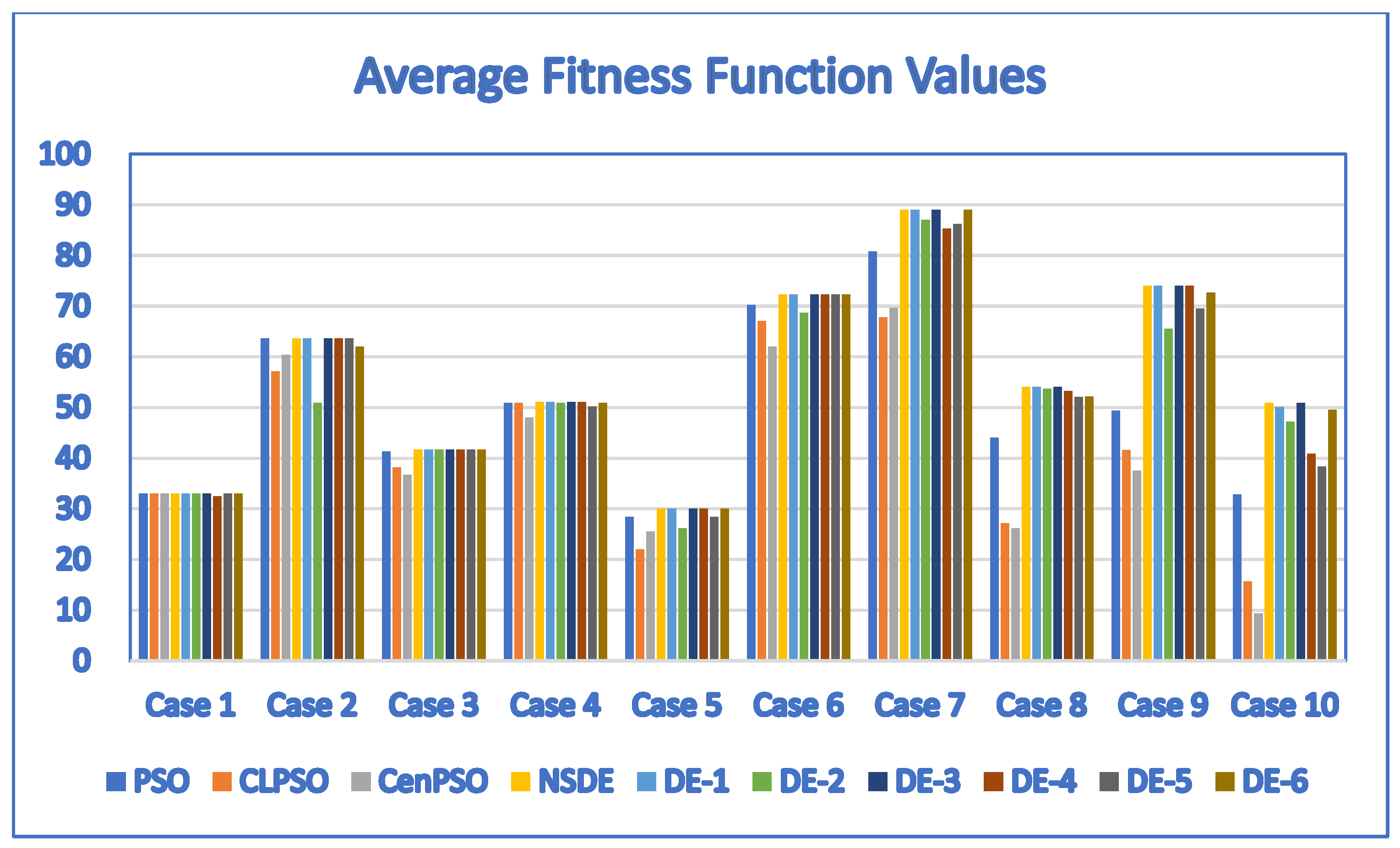
For common parameter setting 1, the population size (POP) was 30. The fitness function values obtained by applying the PSO, CLPSO, CenPSO, and DE-7 (NSDE) algorithms are listed in Table 12. Regarding the three PSO-based algorithms, the average fitness function value obtained by the PSO algorithm was the same as that of the CLPSO algorithm and the CenPSO algorithm for Case 1. The average fitness function values obtained by PSO outperformed those of the CLPSO and CenPSO algorithms for all other cases (Case 2 through Case 10) when the population size was 30.
By comparing the average fitness function values obtained by applying the PSO algorithm and the DE-7(NSDE) algorithm, we found that the average fitness function values obtained by the DE-7(NSDE) algorithm were equal to those of the PSO algorithm for Case 1 and Case 2. Moreover, the fitness function values obtained by the DE-7(NSDE) algorithm were greater than those of the PSO algorithm for all other cases (Case 3 through Case 10). This indicated that the performance of the DE-7(NSDE) algorithm was either as good as the PSO algorithm or better than the PSO algorithm for all test cases when the population size was 30.
When the population size was 30, the average fitness function values obtained by applying the six DE algorithm variations are listed in Table 13. The average fitness function values obtained by the DE-1 algorithm and the DE-3 algorithm were the same as those obtained by the NSDE algorithm for all test cases.
Although the average fitness function values of the DE-2, DE-4, DE-5, and DE-6 algorithms were not as good as those of the NSDE algorithm for all test cases, the average fitness function values obtained by these four DE algorithms were close to those of the NSDE algorithm for most test cases, with some exceptions. The DE-4 and DE-5 algorithms performed poorly in Case 10. In short, the performance of the DE-7(NSDE) algorithm was the same as that of the DE-1 algorithm and the DE-3 algorithm. In addition, the performances of the DE-1, DE-3, and DE-7(NSDE) algorithms were either as good as or better than those of the DE-2, DE-4, DE-5, and DE-6 algorithms for all test cases when the population size was 30.
Based on the analysis above, we found that the DE-1, DE-3, and DE-7(NSDE) algorithms either performed as well as or better than the three variants of the PSO algorithm and the other three DE-based algorithms when the population size was 30. Figure 4 shows the bar chart based on the results listed in Table 12 and Table 13.
We also used the free software KEEL [62] to apply the Friedman test to obtain average rankings for the ten algorithms proposed in this paper based on the results of the experiments for POP = 30 and POP = 50. To perform the Friedman test for the results when POP = 30, the data in Table 12 and Table 13 were first transformed into rank data. Then, the rank data were used as the inputs to perform the Friedman test. The average rankings of the ten algorithms proposed in this paper are shown in Table 14. The results in Table 14 indicate that the best three algorithms were the NSDE, DE-3, and DE-1 algorithms. This was consistent with our analysis. The Friedman statistics showed significant differences between the algorithms, with a value of 48.103636 and a p-value = 0.
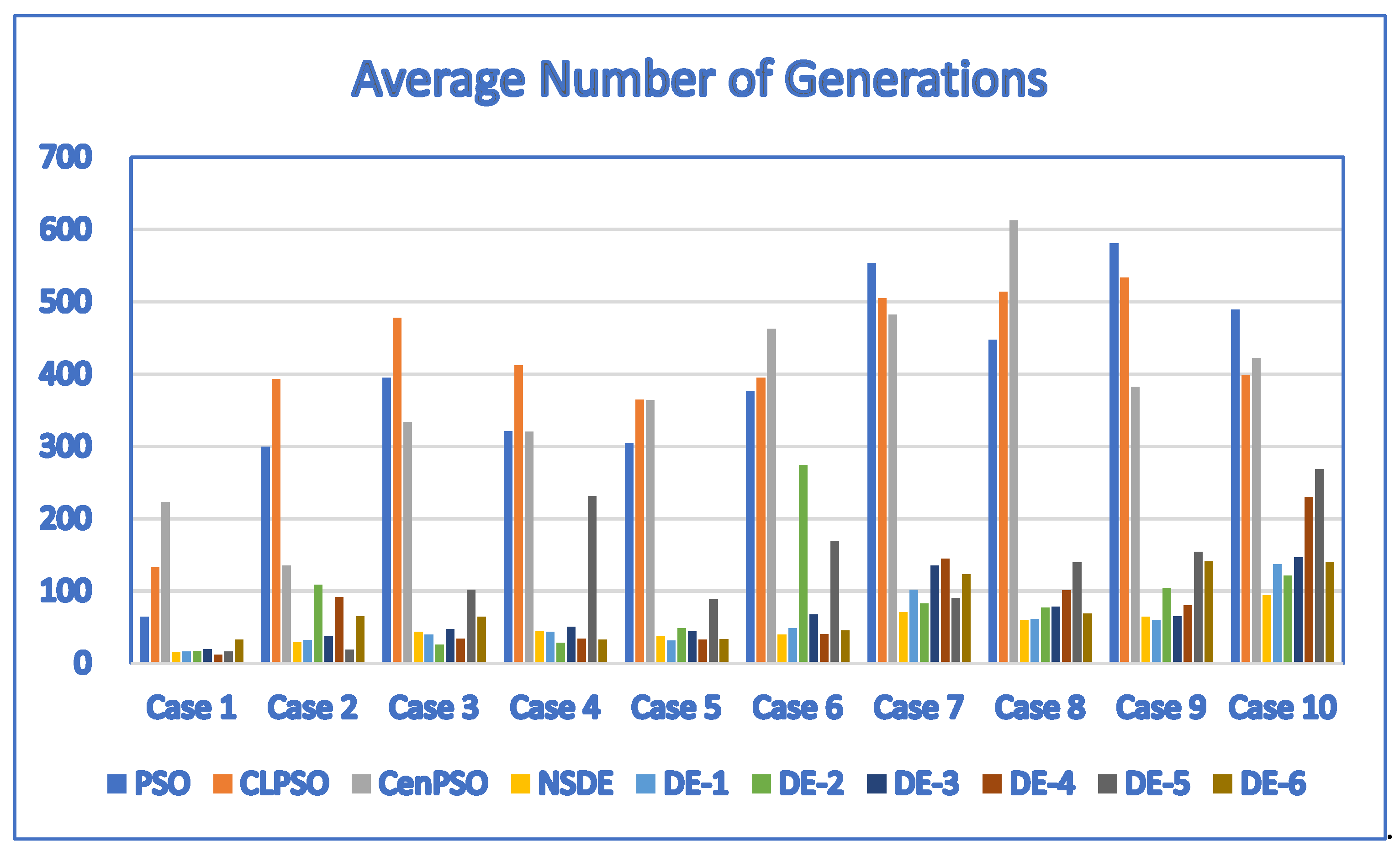
In addition to the comparison of performance based on the average fitness function values, we also compared the efficiency of the ten algorithms. Table 15 and Table 16 show the average number of generations required to find the best solutions for all runs of each algorithm when the population size was 30. Figure 5 shows the average number of generations in a bar chart based on the results listed in Table 15 and Table 16. It can be observed from Table 15 that the average number of generations required to find the best solutions for the DE-7 (NSDE) algorithm was much lower than that of the PSO, CLPSO, and CenPSO algorithms. The DE-7 (NSDE) algorithm was obviously more efficient than the three variants of the PSO algorithm.
By comparing Table 15 with Table 16, it can be seen that the average number of generations required to find the best solutions by the six DE-based algorithms was much lower than that required by the PSO, CLPSO, and CenPSO algorithms. The six DE-based algorithms were more efficient than the three variants of the PSO algorithms when the population size was 30.
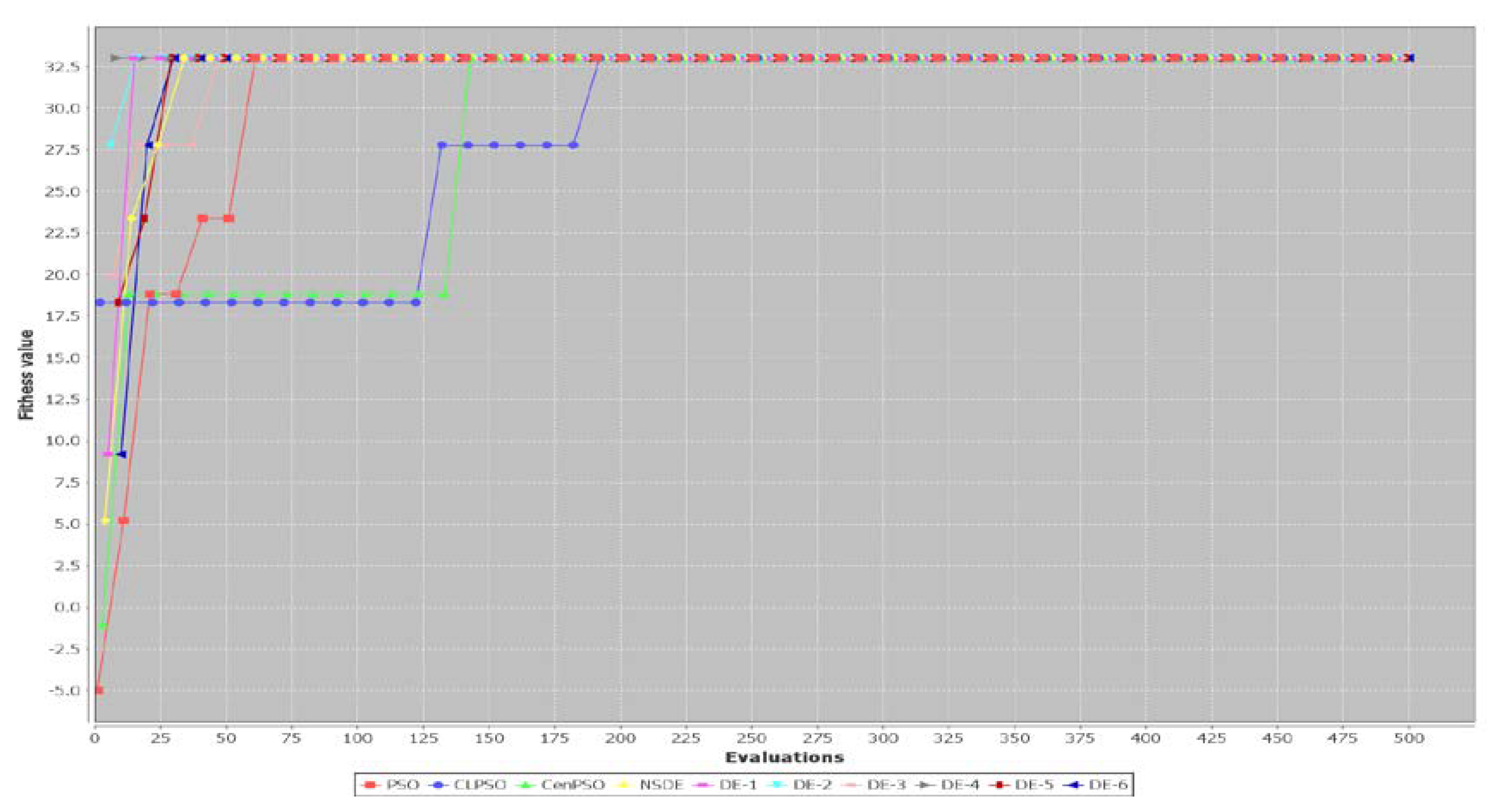
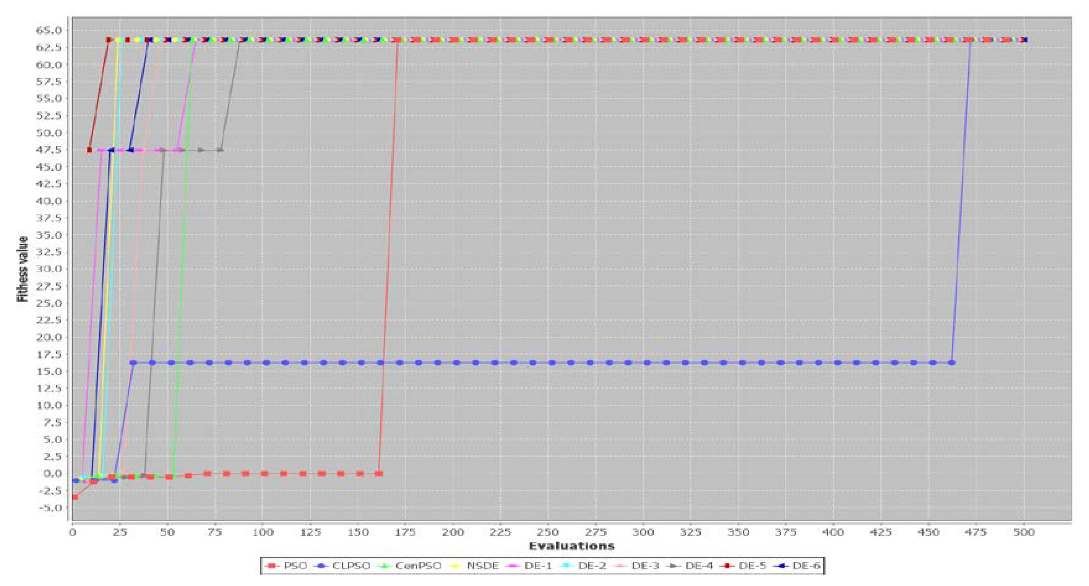
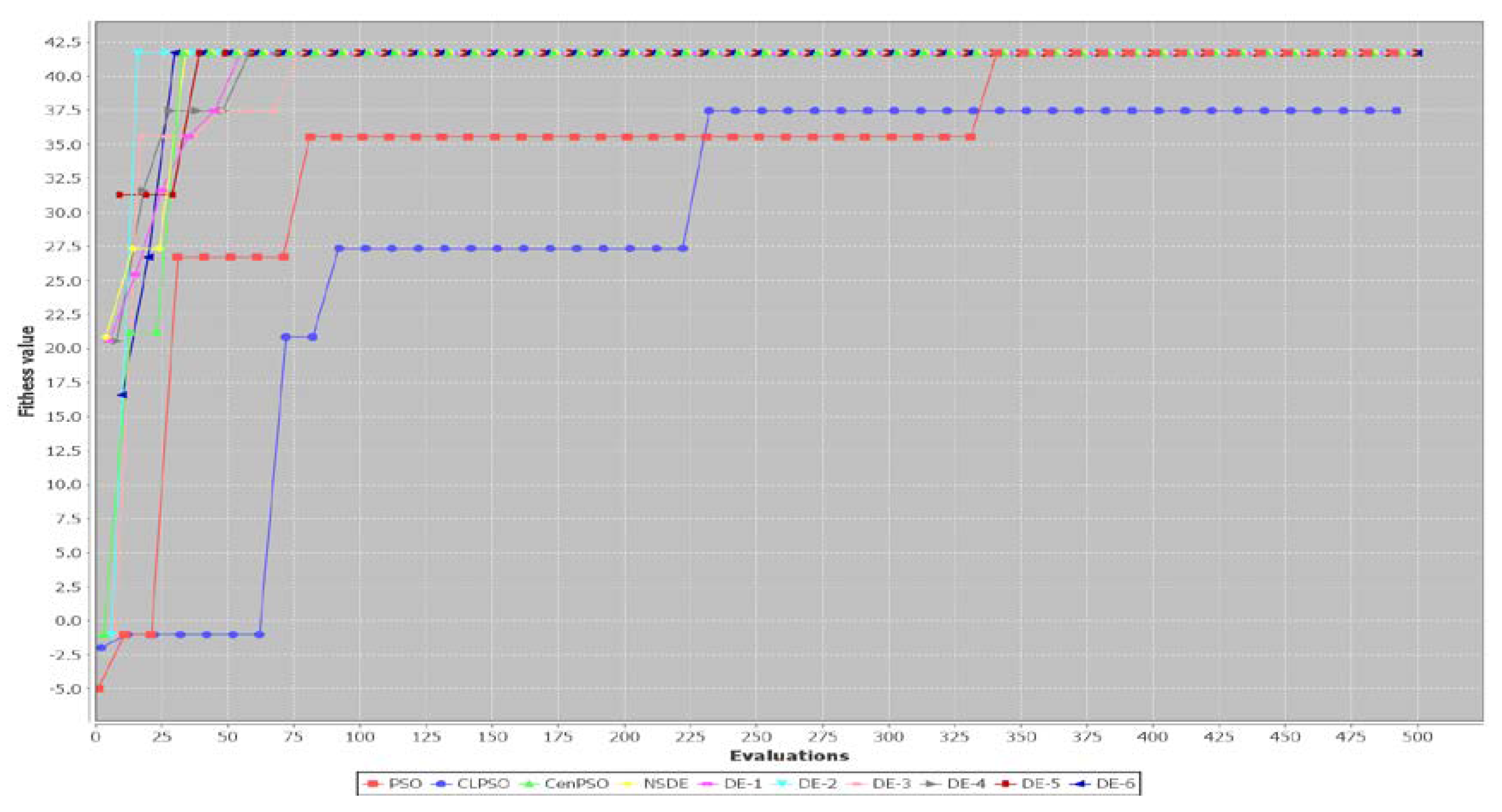
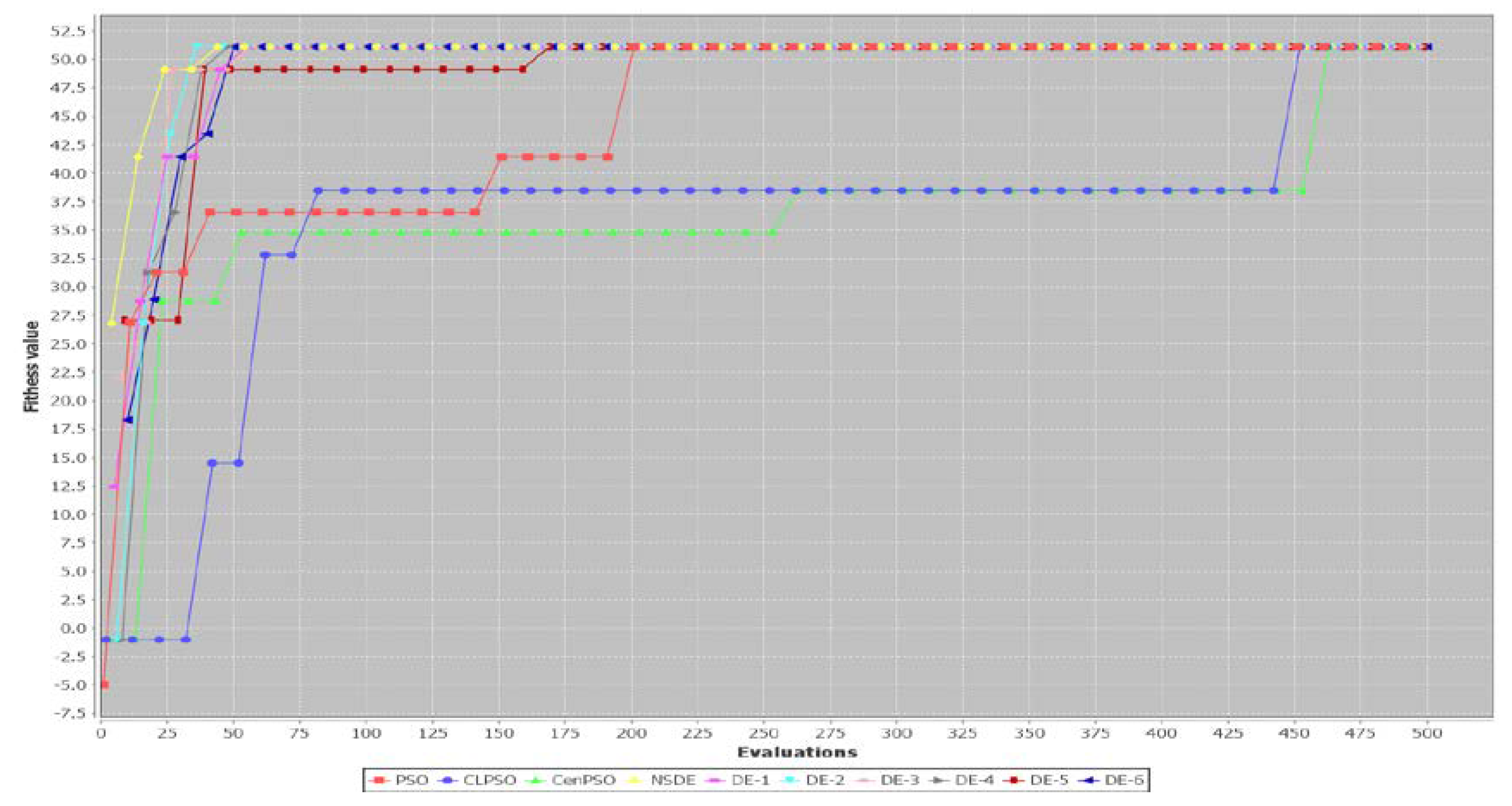
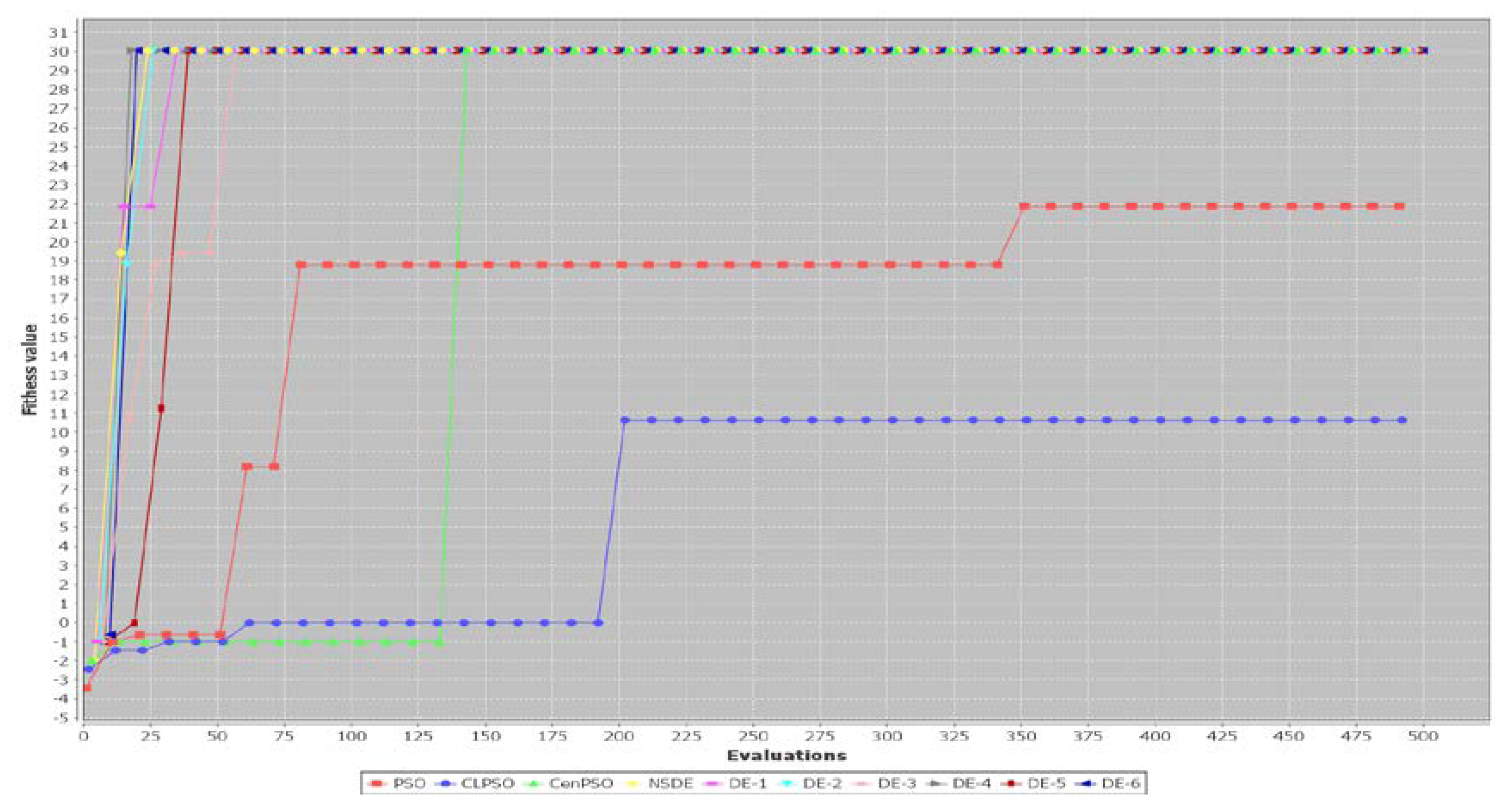
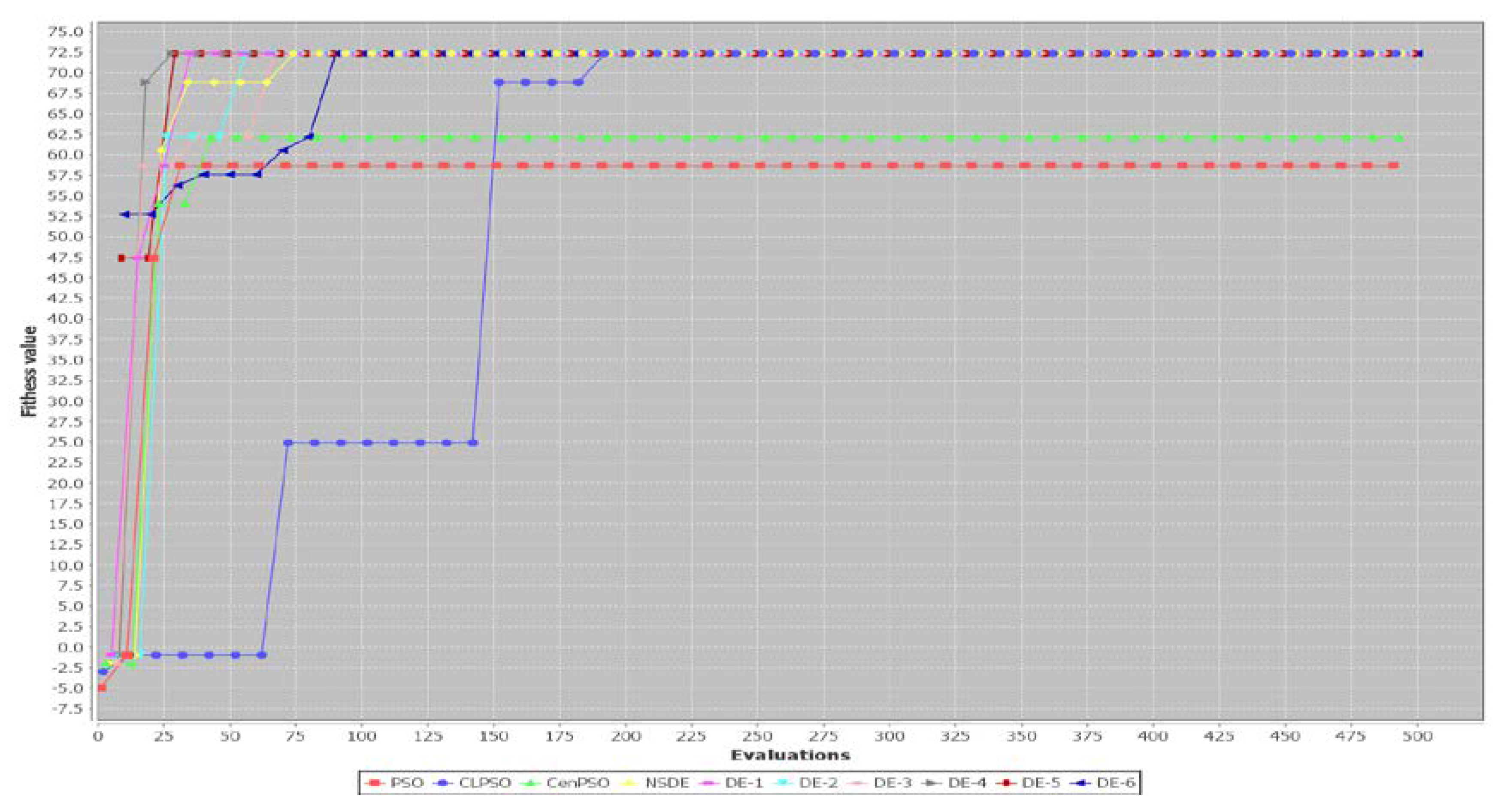
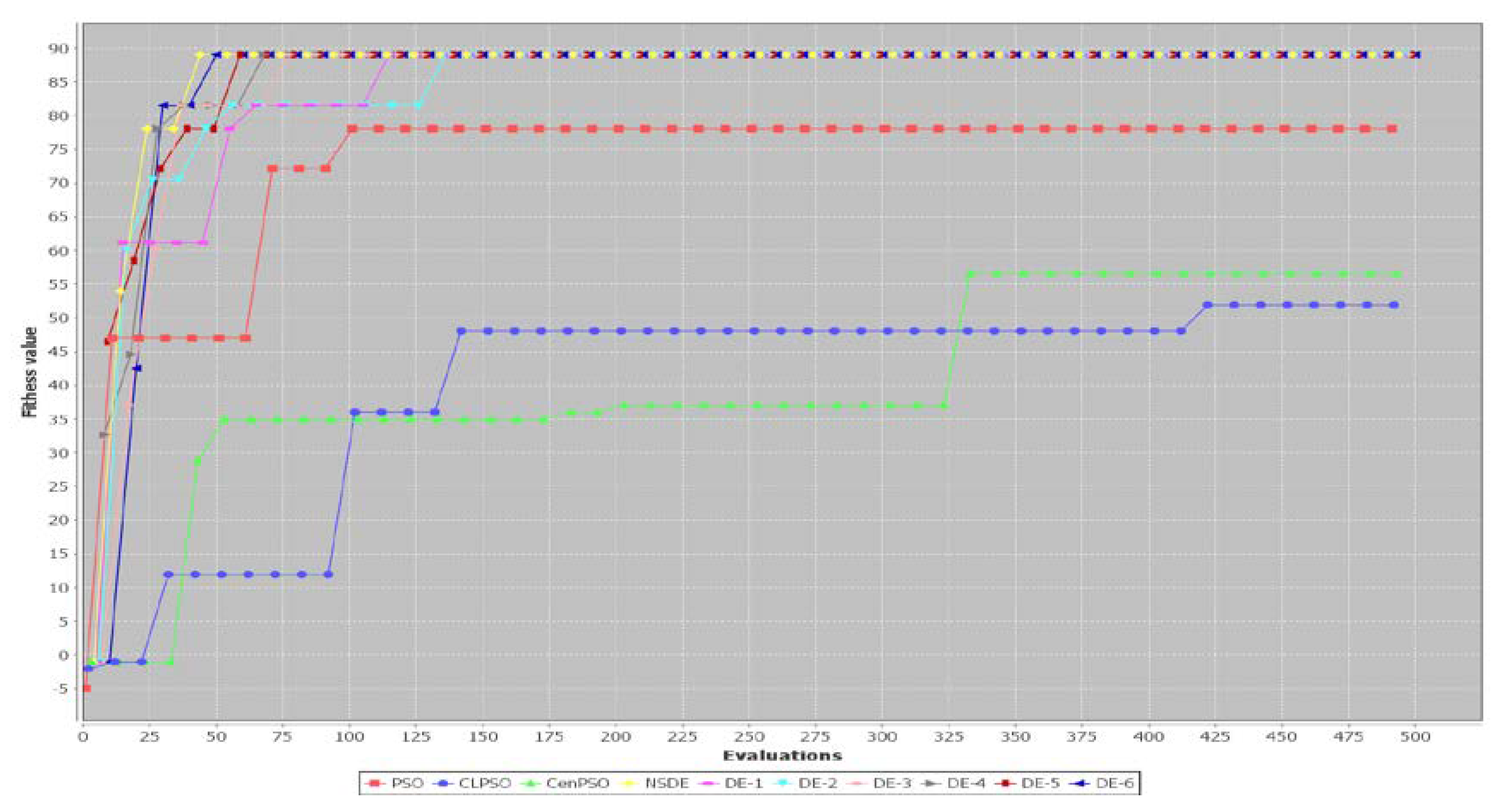
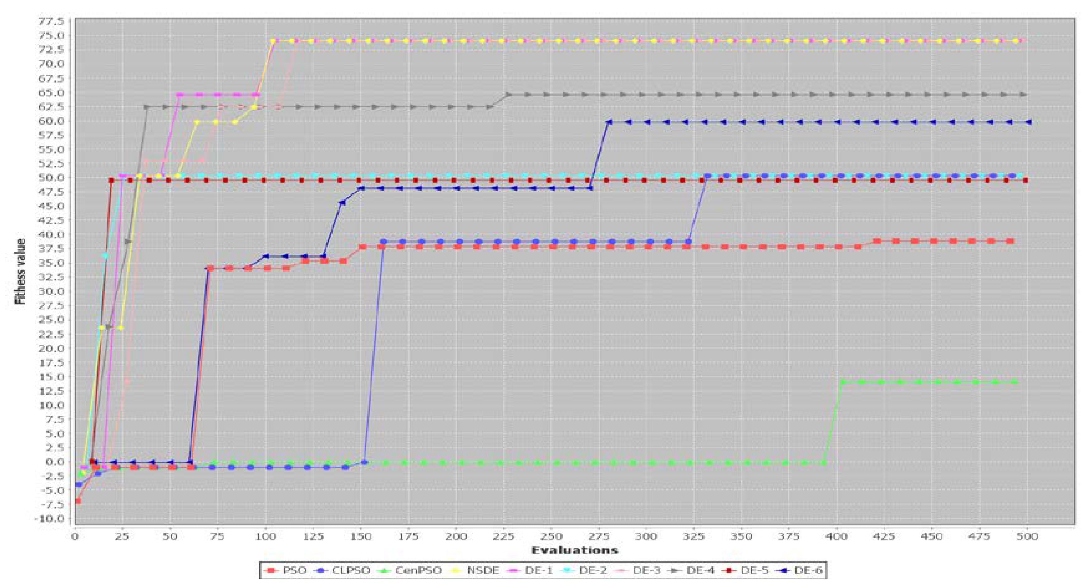
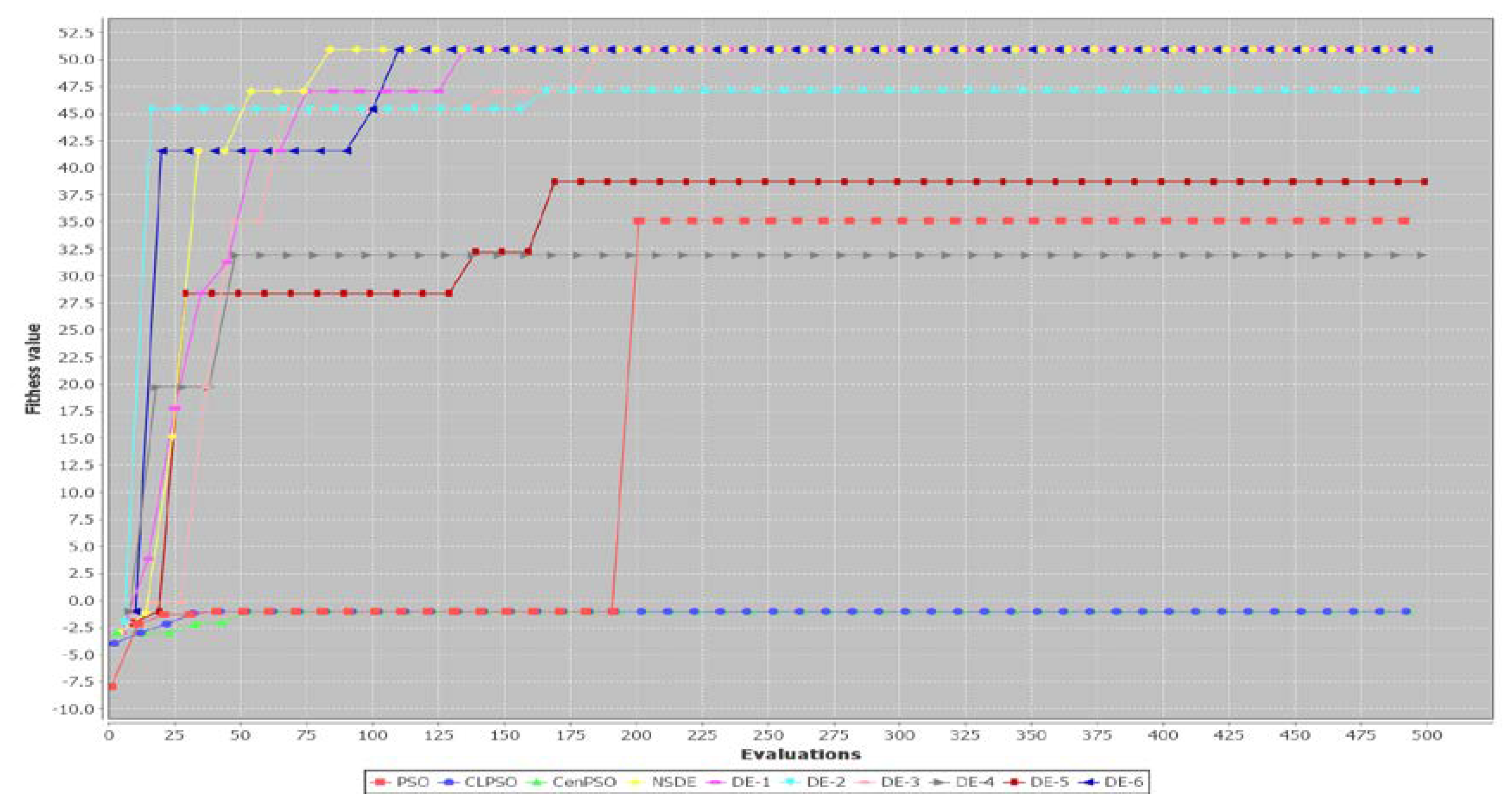
Figure A1 through Figure A10 in Appendix B show the convergence speeds of simulation runs for each algorithm and each test case.
Based on the comparison above, the seven DE-based algorithms were more efficient than the PSO, CLPSO, and CenPSO algorithms when the population size was 30.
For common parameter setting 2, the population size was 50. The average fitness function values obtained by applying the PSO, CLPSO, CenPSO, and DE-7(NSDE) algorithms are listed in Table 17. Regarding the three PSO-based algorithms, the average fitness function value obtained by the PSO algorithm was the same as that of the CLPSO algorithm and the CenPSO algorithm for Case 1. The average fitness function value obtained by the PSO algorithm was also the same as that of the CLPSO algorithm and CenPSO algorithm for Case 2. The average fitness function values obtained by the PSO algorithm were higher than those of the CenPSO algorithm for Case 2. The average fitness function values obtained by the PSO algorithm were higher than those of the CLPSO and CenPSO algorithms for all other cases (Case 3 through Case 10).
By comparing the average fitness function values obtained by the PSO algorithm and the DE-7(NSDE) algorithm, we found that the average fitness function values obtained by the DE-7(NSDE) algorithm were equal to those of the PSO algorithm for Case 1, Case 2, Case 4, and Case 5. Moreover, the average fitness function values obtained by the DE-7(NSDE) algorithm were greater than those of the PSO algorithm for all other cases (Case 3, Case 6, Case 7, Case 8, Case 9, and Case 10). This indicated that the performance of the DE-7(NSDE) algorithm was either as good as or better than that of the PSO algorithm for all the test cases when the population size was 50.
When the population size was 50, the average fitness function values obtained by applying the six DE algorithms are listed in Table 18. The average fitness function values obtained by the DE-1 algorithm and the DE-3 algorithm were the same as those of the NSDE algorithm for all test cases.
Although the average fitness function values of the DE-2, DE-4, DE-5, and DE-6 algorithms were not as good as those of the NSDE algorithm for all test cases, they were close to those of the NSDE algorithm for most test cases, with the exception of Case 10. The DE-4 and DE-5 algorithms performed poorly for Case 10. In short, the performances of the NSDE, DE-1, and DE-3 algorithms were either as good as or better than those of the DE-2, DE-4, DE-5, and DE-6 algorithms for all test cases when the population size was 50.
Based on the analysis above, we found that the DE-1, DE-3, and DE-7(NSDE) algorithms either performed as well as or better than the three variants of the PSO algorithm and the DE-2, DE-4, DE-5, and DE-6 algorithms when the population size was 50. Figure 6 shows the bar chart based on the results listed in Table 17 and Table 18.
We also used the free software KEEL [62] to apply the Friedman test to obtain average rankings for the ten algorithms proposed in this paper based on the results of the experiments for POP = 50. To perform the Friedman test for the results when POP = 50, the data in Table 17 and Table 18 were first transformed into rank data. Then, the rank data were used as the inputs to perform the Friedman test. The average rankings of the ten algorithms proposed in this paper are shown in Table 19. The results in Table 19 indicated that the best three algorithms were the NSDE, DE-3, and DE-1 algorithms. This was consistent with our analysis. The Friedman statistics showed significant differences between the algorithms, with a value of 46.445455 and a p-value = 0.
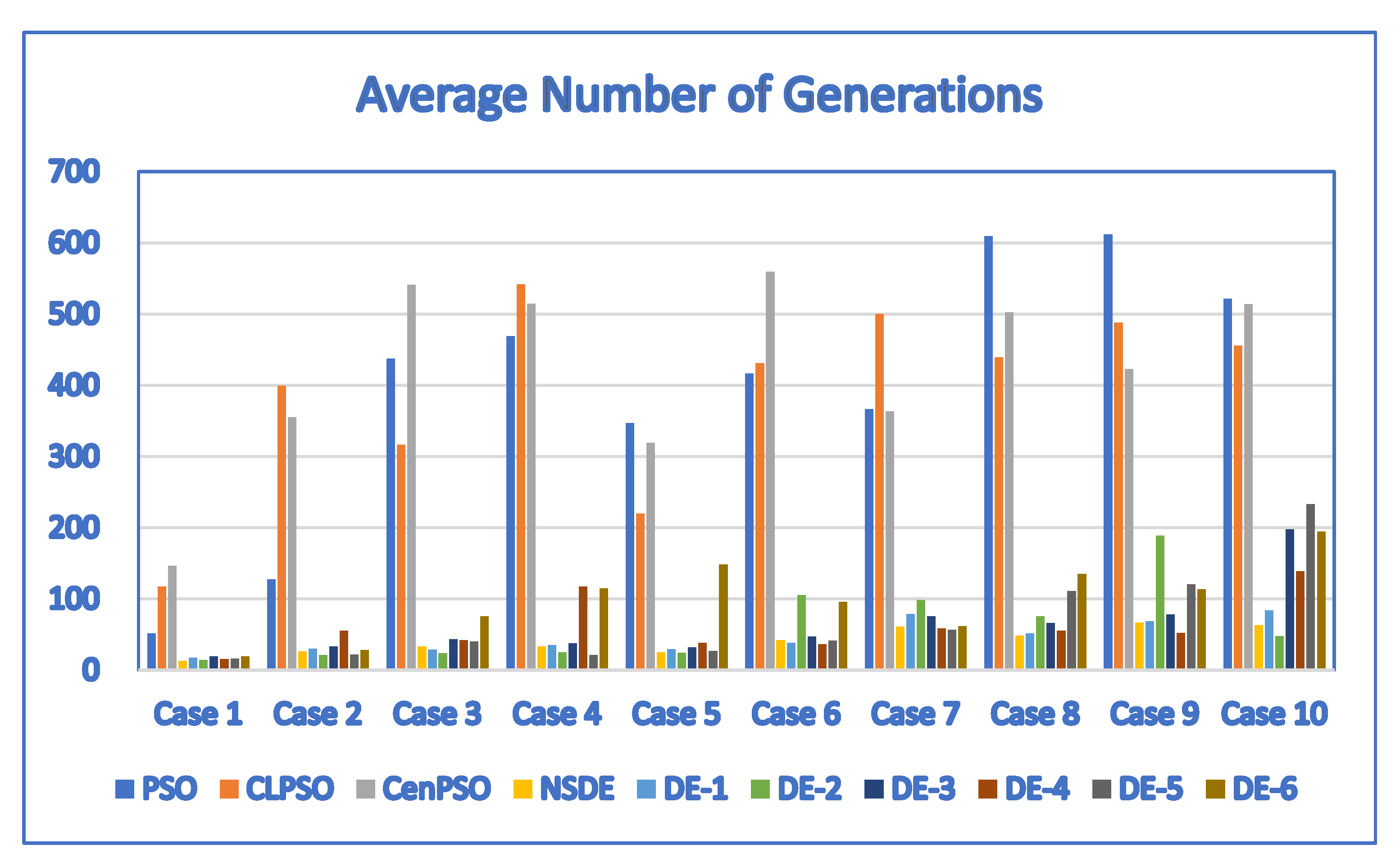
In addition to comparing the performance of the ten algorithms based on the average fitness function values, we also compared their efficiency. Table 20 and Table 21 show the average number of generations required to find the best solutions for all runs of each algorithm when the population size was 50. Figure 7 shows the average number of generations in a bar chart based on the results listed in Table 20 and Table 21. It can be observed from Table 20 that the average number of generations required to find the best solutions for the DE-7 (NSDE) algorithm was much lower than that required by the PSO, CLPSO, and CenPSO algorithms. The DE-7 (NSDE) algorithm was more efficient than the three variants of the PSO algorithm.
By comparing Table 20 with Table 21, it can be seen that the average number of generations required to find the best solutions for the six DE-based algorithms was much smaller than that of the PSO, CLPSO, and CenPSO algorithms. The six DE-based algorithms were more efficient than the three variants of the PSO algorithm when the population size was 50.
Based on the comparison above, the seven DE-based algorithms were more efficient than the PSO, CLPSO, and CenPSO algorithms when the population size was 50.
The above analysis of the POP = 30 and POP = 50 experimental results indicated that the DE-1, DE-3, and DE-7 (NSDE) algorithms were either as good as or outperformed all the other algorithms for the test cases in terms of the average fitness function values. Our analysis also indicated that the DE-1, DE-3, and DE-7 (NSDE) algorithms were much more efficient than the three variants of the PSO algorithm. The efficiency of the DE-1, DE-3, and DE-7 (NSDE) algorithms was comparable to that of the DE-2, DE-4, DE-5, and DE-6 algorithms.

6. Discussion

The results presented in the previous section showed that because the minimal expected cost savings discount parameter was considered in the decision model, it could identify a set of ridesharing participants for whom the minimal cost savings discount was guaranteed to improve user satisfaction with the ridesharing service in terms of cost savings. For example, the small example of Case 1 indicated that the minimal expected cost savings discount could be satisfied for the six ridesharing participants in the solution found by our algorithms. That is, the minimal expected cost savings discount can be guaranteed as long as a solution can be found.
The results presented in the previous section showed that the discount-guaranteed ridesharing problem could be solved by applying different approaches. In this paper, we limited our scope to two approaches: differential evolution and particle swarm optimization. Seven DE-based algorithms and three variants of the PSO algorithm were considered as the candidate solvers to find the solutions for the discount-guaranteed ridesharing problem. Depending on the approach used, the performance and efficiency varied. The seven DE-based algorithms considered in this study followed the same three-step operation process: mutation, crossover, and selection. The differences between these seven DE algorithms lay in the mutation strategies used. The method for improving the quality of a particle in PSO is different to that in DE. In PSO-based approaches, each particle attempts to improve its solution quality by adjusting its velocity. All three variants of the PSO algorithm considered in this study followed the same operation process to determine personal and global bests and update velocity. The differences between these three variants of the PSO algorithm lay in their methods of updating the velocity. Based on the results of our experiments, we compared the average fitness function values and the efficiency of the ten algorithms.
In terms of performance, the average fitness function values obtained by the DE-1, DE-3, and NSDE (DE-7) algorithms were either greater than or the same as those of the other seven algorithms for all the test cases, regardless of whether the population size was 30 or 50. This indicated that the DE-1, DE-3, and NSDE (DE-7) algorithms either performed as well as or better than the other four DE algorithms and the three PSO algorithms for all the test cases, regardless of whether the population size was 30 or 50. In terms of computational efficiency, the analysis of the results indicated that the DE-7 (NSDE) algorithm and all the other DE-based algorithms were more efficient than the three variants of the PSO algorithm for all the test cases when the population size was set to 30 or 50. The efficiency of the DE-7 (NSDE) algorithm was comparable to that of the other six DE algorithms. Overall, the DE-1, DE-3, and DE-7(NSDE) algorithms were the three best choices in terms of performance and computational efficiency for the test cases in this study. This indicated that the minimal cost savings discount constraints had a significant influence on the effectiveness of the evolutionary algorithms.

7. Conclusions

The incentives for users to adopt ridesharing transport modes include monetary incentives and non-monetary incentives. Monetary incentives are mostly related to savings on transport costs, whereas non-monetary incentives may include safety, trust, or enjoyability. In this study, we focused on a monetary incentive issue of ridesharing systems. In the literature, although the problem of optimizing cost savings has been studied extensively, the problem of guaranteeing a minimal cost savings discount for ridesharing participants has been ignored. To bridge this gap, we defined a discount-guaranteed ridesharing problem and proposed a decision model to address this problem. The decision model took into consideration the factor of a minimal cost savings discount. The goal of the decision model was to maximize the total cost savings for ridesharing participants under the constraint that the ridesharing participants’ minimal expected cost savings discount had to be satisfied. Due to the highly non-linear and objective function and constraints, seven DE-based algorithms and three PSO-based algorithms were developed and implemented to solve the decision problem. We illustrated that the proposed method can find a solution that guarantees the satisfaction of the minimal expected cost savings discount. The results were consistent with our expectations. We studied the effectiveness of the ten different algorithms developed based on the DE and PSO approaches. The results indicated that the DE-based algorithm with a neighborhood search mechanism and two other DE algorithms outperformed all the other algorithms used in the experiments. This provided valuable information for selecting the right algorithm to solve a certain type of problem. The contributions of this paper were as follows:
  • The issue of guaranteeing a minimal cost savings discount in ridesharing systems has not been addressed in the literature. Hence, the problem addressed and the decision model proposed in this study differentiate it from our previous studies and other studies in the literature. We proposed a decision model that offers a minimal cost savings discount for drivers and passengers.
  • We proposed ten solution algorithms to provide decision support tools for finding a set of users for whom the minimal cost savings discount can be guaranteed and the total cost savings achieved can be optimized.
  • We provided guidelines for selecting an appropriate solution algorithm by analyzing the results of several test cases and comparing the proposed algorithms.
In this paper, we assumed that the ridesharing information provider was a non-profit organization that aimed to promote ridesharing. The problem formulation can be extended to deal with situations in which a portion of the overall cost savings is allocated to the ridesharing information provider. As many evolutionary algorithms exist, an interesting future research direction would be to study the effectiveness of applying other approaches to solve the problem presented in this paper. We focused on the monetary aspect of ridesharing systems. Other non-monetary issues such as trust were not considered in this paper. A consideration of these issues in a decision model would be an interesting and challenging future research direction. Another challenging future research direction would be to evaluate the feasibility and effectiveness of different cost savings allocation schemes in the discount-guaranteed ridesharing problem.

Funding

This research was supported in part by the National Science and Technology Council, Taiwan, under Grant NSTC 111-2410-H-324-003.

Institutional Review Board Statement

Not applicable for studies not involving humans or animals.

Informed Consent Statement

Not applicable for studies not involving humans.

Data Availability Statement

Data are available in a publicly accessible repository, as described in the article.

Conflicts of Interest

The author declares no conflict of interest.

Appendix A

Procedure RealToBinary
Input: a
Output: c
Step 1:
  • If a > V max
    b V max
  • Else If V max a and a V max
    b a
  • Else
    b V max
  • End If
Step 2: s 1 1 + exp b
Step 3: Generate rsid, a random variable with uniform distribution U(0,1)
  • If r s i d < s
    c 1
  • Else
    c 0
  • End If
  • Return c

Appendix B

Figure A1. Convergence speed of a run of each algorithm for Case 1 with POP = 30.
Applsci 12 09544 g0a1
Figure A2. Convergence speed of a run of each algorithm for Case 2 with POP = 30.
Applsci 12 09544 g0a2
Figure A3. Convergence speed of a run of each algorithm for Case 3 with POP = 30.
Applsci 12 09544 g0a3
Figure A4. Convergence speed of a run of each algorithm for Case 4 with POP = 30.
Applsci 12 09544 g0a4
Figure A5. Convergence speed of a run of each algorithm for Case 5 with POP = 30.
Applsci 12 09544 g0a5
Figure A6. Convergence speed of a run of each algorithm for Case 6 with POP = 30.
Applsci 12 09544 g0a6
Figure A7. Convergence speed of a run of each algorithm for Case 7 with POP = 30.
Applsci 12 09544 g0a7
Figure A8. Convergence speed of a run of each algorithm for Case 8 with POP = 30.
Applsci 12 09544 g0a8
Figure A9. Convergence speed of a run of each algorithm for Case 9 with POP = 30.
Applsci 12 09544 g0a9
Figure A10. Convergence speed of a run of each algorithm for Case 10 with POP = 30.
Applsci 12 09544 g0a10

References

  1. Hyland, M.; Mahmassani, H.S. Operational benefits and challenges of shared-ride automated mobility-on-demand services. Transp. Res. Part A Policy Pract. 2020, 134, 251–270. [Google Scholar] [CrossRef]
  2. Delhomme, P.; Gheorghiu, A. Comparing French carpoolers and non-carpoolers: Which factors contribute the most to carpooling? Transp. Res. Part D Transp. Environ. 2016, 42, 1–15. [Google Scholar] [CrossRef]
  3. Julagasigorn, P.; Banomyong, R.; Grant, D.B.; Varadejsatitwong, P. What encourages people to carpool? A conceptual framework of carpooling psychological factors and research propositions. Transp. Res. Interdiscip. Perspect. 2021, 12, 100493. [Google Scholar] [CrossRef]
  4. Tsai, Y.T.; Yu, C.H.; Boonprakob, R. Assessing carpooling drivers and barriers: Evidence from Bangkok, Thailand. Transp. Res. Part F Traffic Psychol. Behav. 2021, 82, 84–95. [Google Scholar] [CrossRef]
  5. Mitropoulos, L.; Kortsari, A.; Ayfantopoulou, G. A systematic literature review of ride-sharing platforms, user factors and barriers. Eur. Transp. Res. Rev. 2021, 13, 61. [Google Scholar] [CrossRef]
  6. Agatz, N.; Erera, A.; Savelsbergh, M.; Wang, X. Optimization for dynamic ride-sharing: A review. Eur. J. Oper. Res. 2012, 223, 295–303. [Google Scholar] [CrossRef]
  7. Furuhata, M.; Dessouky, M.; Ordóñez, F.; Brunet, M.; Wang, X.; Koenig, S. Ridesharing: The state-of-the-art and future direc-tions. Transp. Res. Part B Methodol. 2013, 57, 28–46. [Google Scholar] [CrossRef]
  8. Ferber, J. Multi-Agent Systems, an Introduction to Distributed Artificial Intelligence; Addison Wesley: Reading, MA, USA, 1999. [Google Scholar]
  9. Nilsson, N.J. Artificial Intelligence: A New Synthesis; Morgan Kaufmann: San Francisco, CA, USA, 1998. [Google Scholar]
  10. De Vries, S.; Vohra, R.V. Combinatorial Auctions:A Survey. INFORMS J. Comput. 2003, 15, 284–309. [Google Scholar] [CrossRef]
  11. Satunin, S.; Babkin, E. A multi-agent approach to Intelligent Transportation Systems modeling with combinatorial auctions. Expert Syst. Appl. 2014, 41, 6622–6633. [Google Scholar] [CrossRef]
  12. Hsieh, F.S.; Zhan, F.; Guo, Y. A solution methodology for carpooling systems based on double auctions and cooperative coevolutionary particle swarms. Appl. Intell. 2019, 49, 741–763. [Google Scholar] [CrossRef]
  13. Rothkopf, M.; Pekeč, A.; Harstad, R. Computationally manageable combinational auctions. Manag. Sci. 1998, 44, 1131–1147. [Google Scholar] [CrossRef]
  14. Xia, M.; Stallaert, J.; Whinston, A.B. Solving the combinatorial double auction problem. Eur. J. Oper. Res. 2005, 164, 239–251. [Google Scholar] [CrossRef]
  15. Price, K.; Storn, R.; Lampinen, J. Differential Evolution: A Practical Approach to Global Optimization; Springer: Berlin/Heidelberg, Germany, 2005. [Google Scholar]
  16. Kennedy, J.; Eberhart, R.C. Particle swarm optimization. In Proceedings of the IEEE International Conference on Neural Networks, Perth, WA, Australia, 27 November–1 December 1995; pp. 1942–1948. [Google Scholar]
  17. Rahmi BA, K.I.; Birgoren, B.; Aktepe, A. Identifying factors affecting intention to use in distance learning systems. Turk. Online J. Distance Educ. 2021, 22, 58–80. [Google Scholar]
  18. Gerte, R.; Konduri, K.C.; Eluru, N. Is There a Limit to Adoption of Dynamic Ridesharing Systems? Evidence from Analysis of Uber Demand Data from New York City. Transp. Res. Rec. 2018, 2672, 127–136. [Google Scholar] [CrossRef]
  19. Sun, Z.; Wang, Y.; Zhou, H.; Jiao, J.; Overstreet, R.E. Travel behaviours, user characteristics, and social-economic impacts of shared transportation: A comprehensive review. Int. J. Logist. Res. Appl. 2021, 24, 51–78. [Google Scholar] [CrossRef]
  20. Abrahamse, W.; Keall, M. Effectiveness of a web-based intervention to encourage carpooling to work: A case study of Wellington. New Zealand. Transp. Policy 2012, 21, 45–51. [Google Scholar] [CrossRef]
  21. Hwang, K.; Giuliano, G. The Determinants of Ridesharing: Literature Review; Working Paper UCTC No. 38; The University of California Transportation Center: Berkeley, CA, USA, 1990; Available online: https://escholarship.org/uc/item/3r91r3r4 (accessed on 10 August 2022).
  22. Liu, K.; Liu, J. Optimization Approach to Improve the Ridesharing Success Rate in the Bus Ridesharing Service. IEEE Access 2020, 8, 208296–208310. [Google Scholar] [CrossRef]
  23. Chen, L.; Zhong, Q.; Xiao, X.; Gao, Y.; Jin, P.; Jensen, C.S. Price-and-Time-Aware Dynamic Ridesharing. In Proceedings of the 2018 IEEE 34th International Conference on Data Engineering (ICDE), Paris, France, 16–19 April 2018; pp. 1061–1072. [Google Scholar]
  24. Hsieh, F.-S. A Hybrid Firefly-DE algorithm for Ridesharing Systems with Cost Savings Allocation Schemes. In Proceedings of the 2022 IEEE World AI IoT Congress (AIIoT), Seattle, WA, USA, 6–9 June 2022; pp. 649–653. [Google Scholar]
  25. Hsieh, F.-S. A Comparison of Three Ridesharing Cost Savings Allocation Schemes Based on the Number of Acceptable Shared Rides. Energies 2021, 14, 6931. [Google Scholar] [CrossRef]
  26. Fu, X. Social-Aware Ridesharing. In Proceedings of the 2019 20th IEEE International Conference on Mobile Data Management (MDM); 2019; pp. 367–368. [Google Scholar]
  27. Guidotti, R.; Sassi, A.; Berlingerio, M.; Pascale, A.; Ghaddar, B. Social or Green? A Data-Driven Approach for More Enjoyable Carpooling. In Proceedings of the 2015 IEEE 18th International Conference on Intelligent Transportation Systems, Gran Canaria, Spain, 15–18 September 2015; pp. 842–847. [Google Scholar]
  28. Hsieh, F.S. Trust-Based Recommendation for Shared Mobility Systems Based on a Discrete Self-Adaptive Neighborhood Search Differential Evolution Algorithm. Electronics 2022, 11, 776. [Google Scholar] [CrossRef]
  29. Braverman, A.; Dai, J.G.; Liu, X.; Ying, L. Empty-Car Routing in Ridesharing Systems. Oper. Res. 2019, 67, 1437–1452. [Google Scholar] [CrossRef]
  30. Fielbaum, A.; Alonso-Mora, J. Unreliability in ridesharing systems: Measuring changes in users’ times due to new requests. Transp. Res. Part C Emerg. Technol. 2020, 121, 102831. [Google Scholar] [CrossRef]
  31. Naoum-Sawaya, J.; Cogill, R.; Ghaddar, B.; Sajja, S.; Shorten, R.; Taheri, N.; Tommasi, P.; Verago, R.; Wirth, F. Stochastic optimization approach for the car placement problem in ridesharing systems. Transp. Res. Part B Methodol. 2015, 80, 173–184. [Google Scholar] [CrossRef]
  32. Thaithatkul, P.; Seo, T.; Kusakabe, T.; Asakura, Y. A passengers matching problem in ridesharing systems by considering user preference. J. East. Asia Soc. Transp. Stud. 2015, 11, 1416–1432. [Google Scholar]
  33. Mourad, A.; Puchinger, J.; Chu, C. A survey of models and algorithms for optimizing shared mobility. Transp. Res. Part B Methodol. 2019, 123, 323–346. [Google Scholar] [CrossRef]
  34. Martins, L.C.; Torre, R.; Corlu, C.G.; Juan, A.A.; Masmoudi, M.A. Optimizing ride-sharing operations in smart sustainable cities: Challenges and the need for agile algorithms. Comput. Ind. Eng. 2021, 153, 107080. [Google Scholar] [CrossRef]
  35. Agatz, N.A.H.; Erera, A.L.; Savelsbergh, M.W.P.; Wang, X. Dynamic ride-sharing: A simulation study in metro Atlanta. Transp. Res. Part B Methodol. 2011, 45, 1450–1464. [Google Scholar] [CrossRef]
  36. Wang, X.; Agatz, N.; Erera, A. Stable Matching for Dynamic Ride-Sharing Systems. Transp. Sci. 2018, 52, 850–867. [Google Scholar] [CrossRef]
  37. Nourinejad, M.; Roorda, M.J. Agent based model for dynamic ridesharing. Transp. Res. Part C Emerg. Technol. 2016, 64, 117–132. [Google Scholar] [CrossRef]
  38. Sun, Y.; Chen, Z.-L.; Zhang, L. Nonprofit peer-to-peer ridesharing optimization. Transp. Res. Part E Logist. Transp. Rev. 2020, 142, 102053. [Google Scholar] [CrossRef]
  39. Tafreshian, A.; Masoud, N. Trip-based graph partitioning in dynamic ridesharing. Transp. Res. Part C Emerg. Technol. 2020, 114, 532–553. [Google Scholar] [CrossRef]
  40. Hsieh, F.S. A Comparative Study of Several Metaheuristic Algorithms to Optimize Monetary Incentive in Ridesharing Systems. ISPRS Int. J. Geo-Inf. 2020, 9, 590. [Google Scholar] [CrossRef]
  41. Lu, M.; Chen, Z.; Shen, S. Optimizing the Profitability and Quality of Service in Carshare Systems Under Demand Uncertainty. Manuf. Serv. Oper. Manag. 2017, 20, 162–180. [Google Scholar] [CrossRef]
  42. Shaheen, S.; Cohen, A. Innovative Mobility: Carsharing Outlook Carsharing Market Overview, Analysis, and Trends; Transportation Sustainability Research Center: Berkeley, CA, USA, 2020; Available online: https://escholarship.org/uc/item/9jh432pm (accessed on 10 August 2022).
  43. Ghallab, M.; Nau, D.S.; Traverso, P. Automated Planning: Theory and Practice, Morgan Kaufmann; Elsevier: Amsterdam, The Netherlands, 2004; ISBN 1-55860-856-7. [Google Scholar]
  44. Smith, R.G. The Contract net protocol: High-level communication and control in a distributed problem solver. IEEE Trans. Comput. 1980, 29, 1104–1113. [Google Scholar] [CrossRef]
  45. Durfee, E.H.; Lesser, V.R. Partial global planning:a coordination framework for distributed hypothesis formation. IEEE Trans. Syst. Man Cybern. 1991, 21, 1167–1183. [Google Scholar] [CrossRef]
  46. Wooldridge, M.; Jennings, N.R. The cooperative problem solving process. J. Log. Comput. 1999, 9, 563–592. [Google Scholar] [CrossRef]
  47. Guajardoa, M.; Ronnqvist, M. A review on cost allocation methods in collaborative transportation. Int. Trans. Oper. Res. 2016, 23, 371–392. [Google Scholar] [CrossRef]
  48. Shapley, L.S. A Value for N-Person Games. A Value N-Pers. Games 1952, 28, 307–317. [Google Scholar] [CrossRef]
  49. Schmeidler, D. The Nucleolus of a Characteristic Function Game. SIAM J. Appl. Math. 1969, 17, 1163–1170. [Google Scholar] [CrossRef]
  50. Kalai, E. Proportional solutions to bargaining situations: Intertemporal utility comparisons. Econometrica 1977, 45, 1623–1630. [Google Scholar] [CrossRef]
  51. Fatima, S.S.; Wooldridge, M.; Jennings, N.R. A linear approximation method for the Shapley value. Artif. Intell. 2008, 172, 1673–1699. [Google Scholar] [CrossRef]
  52. Perea, F.; Puerto, J. A heuristic procedure for computing the nucleolus. Comput. Oper. Res. 2019, 112, 104764. [Google Scholar] [CrossRef]
  53. Baki, R. An integrated, multi-criteria approach based on environmental, economic, social, and competency criteria for supplier selection. RAIRO-Oper. Res. 2021, 55, 1487–1500. [Google Scholar] [CrossRef]
  54. Majumder, S.; Saha, B.; Anand, P.; Kar, S.; Pal, T. Uncertainty based genetic algorithm with varying population for random fuzzy maximum flow problem. Expert Syst. 2018, 35, e12264. [Google Scholar] [CrossRef]
  55. Cao, Y.; Zhang, H.; Li, W.; Zhou, M.; Zhang, Y.; Chaovalitwongse, W.A. Comprehensive Learning Particle Swarm Optimization Algorithm With Local Search for Multimodal Functions. IEEE Trans. Evol. Comput. 2019, 23, 718–731. [Google Scholar] [CrossRef]
  56. Mousavirad, S.J.; Rahnamayan, S. CenPSO: A Novel Center-based Particle Swarm Optimization Algorithm for Large-scale Optimization. In Proceedings of the 2020 IEEE International Conference on Systems, Man, and Cybernetics (SMC), Toronto, ON, Canada, 11–14 October 2020; pp. 2066–2071. [Google Scholar]
  57. Yang, Z.; He, J.; Yao, X. Making a difference to differential evolution. In Advances in Metaheuristics for Hard Optimization; Michalewicz, Z., Siarry, P., Eds.; Springer: Berlin, Germany, 2007; pp. 415–432. [Google Scholar]
  58. Ravindran, A.; Ragsdell, K.M.; Reklaitis, G.V. Enginering Optimization: Methods and Applications, 2nd ed.; Wiley: Hoboken, NJ, USA, 2007. [Google Scholar]
  59. Deb, K. Optimization for Engineering Design: Algorithms and Examples; Prentice-Hall: Hoboken, NJ, USA, 2004. [Google Scholar]
  60. Deb, K. An efficient constraint handling method for genetic algorithms. Comput. Methods Appl. Mech. Eng. 2000, 186, 311–338. [Google Scholar] [CrossRef]
  61. Data of Test Cases. Available online: https://drive.google.com/drive/folders/19Zj69lRsQP8z0uuiJOqfkHBegCvZE2Pe?usp=sharing (accessed on 11 August 2022).
  62. Triguero, S.; González, J.M.; Moyano, S.; García, J.; Alcalá-Fdez, J.; Luengo, A.; Fernández, M.J.; del Jesus, L.; Sánchez, L.; Herrera, F. KEEL 3.0: An Open Source Software for Multi-Stage Analysis in Data Mining. Int. J. Comput. Intell. Syst. 2017, 10, 1238–1249. [Google Scholar] [CrossRef] [Green Version]
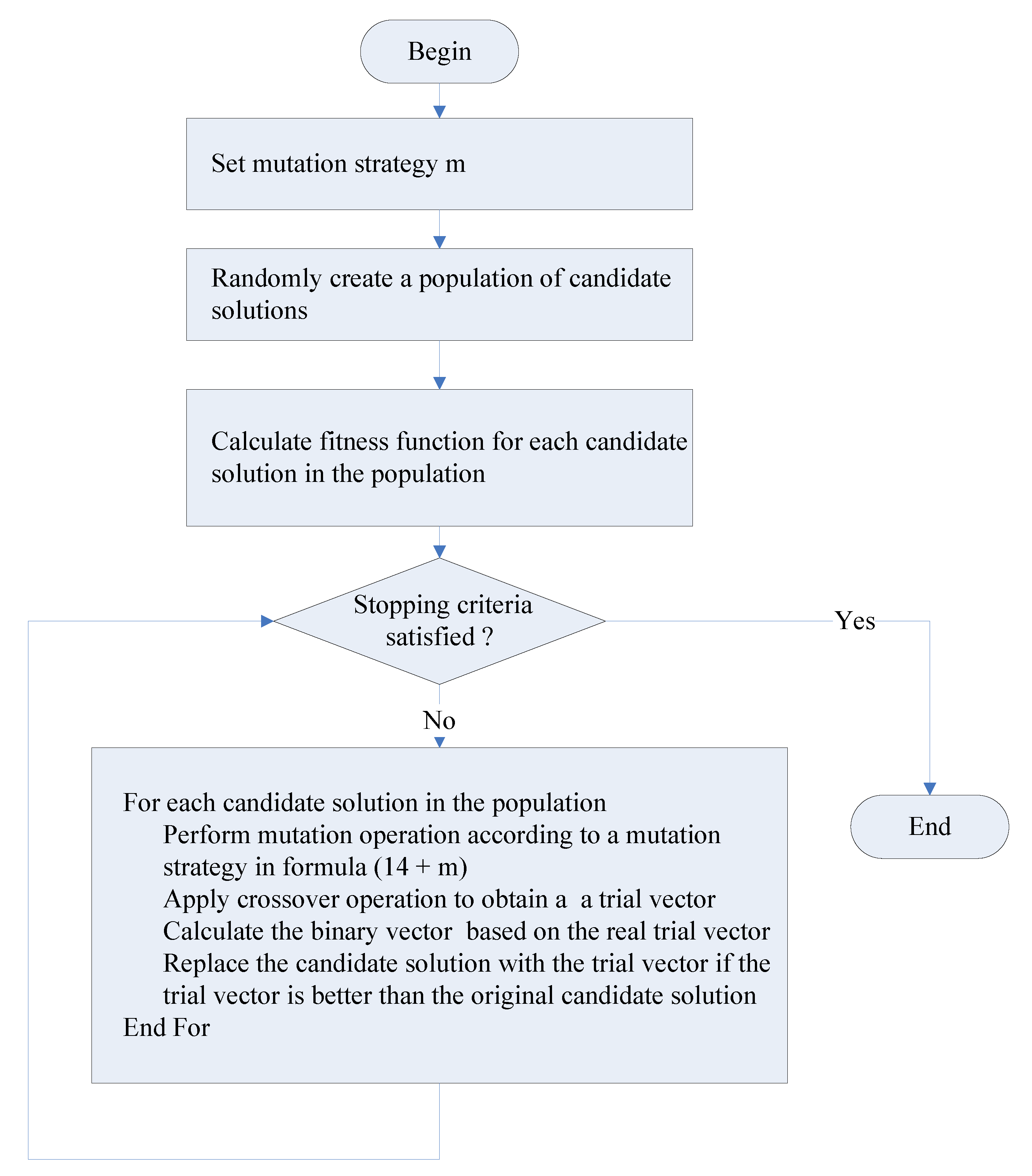
Figure 1. A flow chart for the DE-m algorithm with mutation strategy m.
Applsci 12 09544 g001
Figure 2. A flow chart for the three variants of the PSO algorithm with velocity update strategy v.
Applsci 12 09544 g002
Figure 3. Results shown on a map.
Applsci 12 09544 g003
Figure 4. Average fitness function values for rD = rP = 0.1 when NP = 30.
Applsci 12 09544 g004
Figure 5. Average number of generations for rD = rP = 0.1 with NP = 30.
Applsci 12 09544 g005
Figure 6. Average fitness function values for rD = rP = 0.1 with NP = 50.
Applsci 12 09544 g006
Figure 7. Average number of generations for rD = rP = 0.1 when NP = 50.
Applsci 12 09544 g007
Table 1. Notations of symbols, variables, and parameters.
VariableMeaning
PTotal no. of passengers.
DTotal no. of drivers.
p The   index   of   a   passenger   and   the   corresponding   passenger   agent ,   where   p { 1 , 2 , 3 , P } .
d The   index   of   a   driver   and   the   corresponding   driver   agent ,   where   d { 1 , 2 , 3 , , D } .
k The   index   of   a   location ,   k { 1 , 2 , , K } .
Jd Total   no .   of   bids   submitted   by   driver   agent   d { 1 , 2 , , D } .
j The   index   of   the   j - th   bid   placed   by   a   driver   agent   with   j { 1 , 2 , , J d } .
DBdjDBdj = (qdj1, qdj2, qdj3, …, qdjP, odj, cdj): the j-th bid of driver agent d, where
qdjp is the available seats to serve passenger p,
odj is the original cost when the driver travels alone, and
cdj is the travel cost of the bid.
q d j p 1 The   number   of   seats   for   picking   up   passengers   at   the   pick - up   location   of   passenger   p ,   q d j p 1 = q d j p .
q d j p 2 The   number   of   seats   released   after   dropping   the   passengers   at   the   drop - off   location   of   passenger   p ,   q d j p 2 = q d j p .
PBpPBp = (Sp1, Sp2, Sp3, …, SpK, fp): the bid of passenger agent p, where
Spk is the number of seats requested by passenger p for location k and
fp is the cost of passenger p without ridesharing.
s p k 1 No .   of   seats   requested   by   passenger   p   at   the   pick - up   location   of   passenger   p ,   s p k 1 = { s p p   i f   k = p 0   o t h e r w i s e .
s p k 2 No .   of   seats   requested   by   passenger   p at   the   drop - off   location   of   passenger   p ,   s p k 2 = { s p p   i f   k = p 0   o t h e r w i s e   .
xdjA decision variable: xdj = 1 if the j-th bid of driver d is a winning bid and xdj = 0 otherwise.
ypA binary decision variable: yp = 1 if the bid of passenger p is a winning bid and yp = 0 otherwise.
rDMinimal expected cost savings discount for drivers.
rPMinimal expected cost savings discount for passengers.
H(x,y)The total cost savings objective function,
H ( x , y ) = ( p = 1 P y p ( f p ) ) + ( d = 1 D j = 1 J d x d j o d j ) -   ( d = 1 D j = 1 J d x d j c d j ) .
Γ d j The set of passengers on the ride corresponding to the j-th bid submitted by driver d.
Hdj(x,y)The cost savings of the j-th bid submitted by driver d
H d j ( x , y ) = [ ( p Γ d j y p f p ) + x d j o d j -   ( x d j c d j ) ] .
cfpdj Travel   cos t   for   passenger   p   on   the   ride   corresponding   to   the   j - th   bid   submitted   by   driver   d ,   where   p Γ d j .
Table 2. Notations of symbols, variables, and parameters used in the seven DE algorithms.
VariableMeaning
N Dimension   of   the   problem ,   N = d = 1 D J d + P .
mA mutation strategy.
NPPopulation size.
GNumber of generations.
tThe generation index.
ziThe i–th candidate solution in the population.
FiScale factor of individual i.
CRCrossover rate of individual i.
viA mutant vector.
uiA trial vector.
u ¯ i The transformed binary trial vector corresponding to ui.
zbThe best candidate solution in the current population.
zrA candidate solution randomly selected from the population, where r is a random integer between 1 and NP.
r1, r2, r3, r4, r5Random integers between 1 and NP.
N ( μ , σ 1 2 ) A   random   variable   with   Gaussian   distribution   N ( μ , σ 1 2 ) ,   where   the   mean   is   μ   and   the   standard   deviation   is   σ 1 .
Table 3. Notations of symbols, variables, and parameters used in the three PSO algorithms.
VariableMeaning
N The   problem   dimension ,   N = d = 1 D J d + P .
mA mutation strategy.
NPPopulation size.
SThe number of particles randomly selected from the population.
GNumber of generations.
tThe generation index.
ziThe i-th candidate solution in the population.
P z i The   personal   best   of   particle   i ,   where   i { 1 , 2 , , N P } ,   and   P z i n   is   the   n - th   element   of   the   vector   P z i ,   where   n { 1 , 2 , , N } .
GZ The   global   best ,   with   G z n   being   the   n - th   element   of   the   vector   G Z ,   where   n { 1 , 2 , , N } .
viThe velocity of particle i; vin denotes the n-th element of the vector vi.
c1, c2, c3Non-negative real parameters less than 1.
r1, r2, r3Random variables with uniform distribution U(0,1).
Table 4. Start locations and end locations of drivers.
DriverStart Location
(Latitude/Longitude)
Destination Location
(Latitude/Longitude)
Driver 124.23785/120.6699324.11308/120.65914
Driver 224.1692536/120.684823324.20195/120.56815
Driver 324.13425/120.553924.14289/120.70549
Table 5. Start locations and end locations of passengers.
DriverStart Location
(Latitude/Longitude)
Destination Location
(Latitude/Longitude)
Passenger 124.21872/120.646924.12877/120.66223
Passenger 224.1790507/120.665747624.17369/120.61354
Passenger 324.0611/120.6434224.1465287/120.6532456
Passenger 424.07962/120.6945424.12438/120.66244
Passenger 524.19422/120.6953824.15288/120.69704
Passenger 624.16048/120.6917324.16359/120.65138
Passenger 724.0611/120.6434224.11009/120.64146
Passenger 824.19422/120.6953824.13046/120.7047
Passenger 924.13623/120.6069324.13527/120.6571
Passenger 1024.16429/120.6852224.15345/120.65495
Table 6. The number of seats in the bids submitted by drivers.
Driver ID (d)j q d j 1 q d j 2 q d j 3 q d j 4 q d j 5 q d j 6 q d j 7 q d j 8 q d j 9 q d j 10 Γ d j
110000100000{ 5 }
210000000001{ 10 }
310000000010{ 9 }
Table 7. Price information in the bids submitted by drivers.
Driver ID (d)jodjcdj
1150.402551.4975
2136.74541.1575
3157.48557.485
Table 8. Bids submitted by passengers.
Passenger ID (p) s p 1 s p 2 s p 3 s p 4 s p 4 s p 4 s p 4 s p 4 s p 4 s p 4 f p
1100000000037.0475
2010000000018.3475
3001000000028.12
4000100000019.07
5000010000014.1675
6000001000012.25
7000000100017.1175
8000000010033.11
9000000001014.6925
1000000000019.645
Table 9. Solution x for drivers when rD = rP = 0.1.
Driver Decision Variablex11x21x31
Value111
Table 10. Solution y for passengers when rD = rP = 0.1.
Passenger Decision Variabley1y2y3y4y5y6y7y8y9y10
Value0000100011
Table 11. Parameters of each algorithm.
AlgorithmAlgorithm-Specific ParametersCommon Parameter
Setting 1
Common Parameter Setting 2
PSO c 1 = 0.4 , c 2 = 0.6 , ω = 0.4 POP = 30, Gen = 1000POP = 50, Gen = 1000
CLPSO c 1 = 0.4 , c 2 = 0.6 , ω = 0.4 , p c = 0.5 POP = 30, Gen = 1000POP = 50, Gen = 1000
CenPSO c 1 = 0.4 , c 2 = 0.6 , c 3 = 0.6 , ω = 0.4 POP = 30, Gen = 1000POP = 50, Gen = 1000
DE-m
( m { 1 , 2 , 3 , 4 , 5 , 6 } )
CR = 0.5
Fi: a value arbitrarily selected from uniform (0, 2)
POP = 30, Gen = 1000POP = 50, Gen = 1000
DE-7
(NSDE)
CR = 0.5; Fi = 0.5r1 + 0.5, where r1 is a random value with Gaussian distribution N(0,1).POP = 30, Gen = 1000POP =50, Gen =1000
Table 12. Fitness function values for discrete PSO, CLPSO, CenPSO, and DE-7 (NSDE) algorithms with NP = 30; rD = rP = 0.1.
CaseDPPSOCLPSOCenPSODE-7
(NSDE)
131032.99832.99832.99832.998
251163.61557.126260.370663.615
351241.289238.192836.692241.715
461250.908550.908547.995851.11
571328.425421.963525.48230.063
681470.262967.056162.000172.328
791580.810667.756269.655189.03
8101644.002327.118926.187754.02
9111749.35641.621137.505774.05
10121832.834915.66449.36150.9
Table 13. Fitness function values for six discrete DE algorithms with population size NP = 30; rD = rP = 0.1.
CaseDPDE-1DE-2DE-3DE-4DE-5DE-6
131032.99832.99832.99832.474732.99832.998
251163.61550.892263.61563.61563.61561.9928
351241.71541.71541.71541.71541.71541.715
461251.1150.908551.1151.1150.14150.9085
571330.06326.137930.06330.06328.425430.063
681472.32868.661472.32872.32872.32872.328
791589.0386.989889.0385.32386.21389.03
8101654.0253.704654.0253.223552.053152.1271
9111774.0565.566674.0574.0569.486472.6228
10121850.062347.162350.940.911938.357149.5823
Table 14. Average rankings of the ten algorithms obtained by Friedman test for NP = 30.
AlgorithmRanking
PSO6.85
CLPSO8.55
CenPSO9.1
NSDE3
DE-13.15
DE-26.25
DE-33
DE-44.7
DE-55.75
DE-64.65
Table 15. Average number of generations for PSO, CLPSO, CenPSO, and DE-7 (NSDE) algorithms with NP = 30; rD = rP = 0.1.
CaseDPPSOCLPSOCenPSODE-7
(NSDE)
131064.6132.5222.715.6
2511299.6392.6134.929.1
3512394.5477.9333.443.3
4612320.9411.932044.1
5713304.1364.4363.737.3
6814375.6394.9462.539.6
7915553.6505.148270.7
81016447.5513.6612.659.5
91117580.7533.3382.364.2
101218489.3397.8421.994.3
Table 16. Average number of generations for six discrete DE algorithms with population size NP = 30; rD = rP =0.1.
CaseDPDE-1DE-2DE-3DE-4DE-5DE-6
131016.616.719.811.916.432.9
251132.2108.536.991.318.665.3
351239.72647.633.9101.964.6
461243.828.350.334.3231.232.6
571331.848.544.132.788.733.7
681448.327467.840.3169.145.5
7915101.482.9135144.890.3122.9
8101661.377.278.6101.1139.769
9111759.7103.36580.1154.3140.8
101218136.8121.1146.3229.7268.6140.2
Table 17. Fitness function values for discrete PSO, CLPSO, CenPSO, and DE-7 (NSDE) algorithms with NP = 50; rD = rP = 0.1.
CaseDPPSOCLPSOCenPSODE-7
(NSDE)
131032.99832.99832.99832.998
251163.61563.61558.748463.615
351241.289240.246440.011841.715
461251.1149.242550.70751.11
571330.06327.300126.787830.063
681469.948365.576268.285472.328
791580.598676.152275.20789.03
8101646.801334.971834.54454.02
9111755.935640.20151.273674.05
10121831.113119.740320.541750.9
Table 18. Fitness function values for six discrete DE algorithms with population size NP = 50; rD = rP = 0.1.
CaseDPDE-1DE-2DE-3DE-4DE-5DE-6
131032.99832.99832.99832.99832.99832.998
251163.61558.875863.61563.61563.61561.9928
351241.71540.278541.71541.71541.289241.715
461251.1151.1151.1148.393151.1151.11
571330.06330.06330.06330.06330.06330.063
681472.32868.473872.32872.32872.32872.328
791589.0384.733189.0389.0388.277888.091
8101654.0252.269354.0253.862353.862352.4425
9111774.0568.167874.0573.103368.286371.9426
10121850.950.347750.944.977349.317737.2349
Table 19. Average rankings of the ten algorithms obtained by Friedman test for NP = 50.
AlgorithmRanking
PSO6.65
CLPSO8.75
CenPSO9.05
NSDE3.2
DE-13.2
DE-26.4
DE-33.2
DE-44.65
DE-55.15
DE-64.75
Table 20. Average number of generations for discrete PSO, CLPSO, CenPSO, and DE-7 (NSDE) algorithms with NP = 50; rD = rP = 0.1.
CaseDPPSOCLPSOCenPSODE-7
(NSDE)
131051.5117.3146.612.9
2511127.3399.335526.4
3512437.2316.6540.732.9
4612468.6541.4514.633.2
5713347.1219.9319.324.8
6814416.4431.1559.341.9
7915366.4499.8363.661.3
81016609.5438.9502.148.6
91117611.5487.6422.867
101218521.5455.6513.663.1
Table 21. Average number of generations for six discrete DE algorithms with population size NP = 50; rD = rP = 0.1.
CaseDPDE-1DE-2DE-3DE-4DE-5DE-6
131017.61419.215.516.219.2
251130.221.23355.322.128
351228.723.743.341.940.175.7
461235.425.237.4117.321.4114.7
571329.324.332.238.126.7148.6
681438105.247.136.641.796
791578.998.275.458.756.761.9
8101651.575.766.355.6110.7135.3
9111768.7188.578.451.9120.2113.6
10121883.647.9197.9138.7233.2194.2
Publisher’s Note: MDPI stays neutral with regard to jurisdictional claims in published maps and institutional affiliations.