Adaptive Robust Fuzzy Impedance Control of an Electro-Hydraulic Actuator

Abstract

This paper concentrates on both velocity and force control of a single-rod electro-hydraulic actuator in the presence of parameter uncertainties and uncertain nonlinearities. Both velocity control and force control are required in some cases. Impedance control and adaptive robust control are synthesized to deal with this problem. In this paper, the primary goal is velocity control while the contact force is kept in an acceptable range. To keep proper contact force with environment or workpieces, impedance control is adopted to regulate the dynamic relationship between velocity and force. Fuzzy logic is used to adjust the parameters of impedance rules to improve control performance. The velocity command of adaptive robust velocity control is determined by impedance control based on fuzzy logic. Parameter uncertainties and uncertain nonlinearities can be compensated through adaptive robust velocity control, which leads to accurate velocity tracking. The stability of the overall system was analyzed. Comparative experiments verified that the proposed control strategy has both high-accuracy velocity tracking and force regulation performance.

1. Introduction

Electro-hydraulic systems play an important role in construction vehicles, industrial applications, and underwater operations. Accurate velocity control is necessary, e.g., hydraulic elevators [1,2]. Accurate force control is also required, e.g., load simulators [3,4]. Both velocity and force control are required in robot manipulators [5,6,7,8], underwater manipulators [9,10] and tunnel boring machines [11,12]. It is necessary to keep an expected dynamic balance between the motion of the actuator and the contact force with the environment or workpieces.

Hogan [13,14,15] developed impedance control to deal with the dynamics between the actuator and the environment. Impedance control adjusts the dynamic relationship between the position and force of the end effector as a mass-damper-spring system. After this, many researchers paid attention to impedance control. Jamwal et al. [16] developed an impedance control strategy for a lightweight intrinsically compliant parallel ankle rehabilitation robot powered by pneumatic muscle actuators. Hyun et al. [17] implemented proprioceptive impedance control in the MIT Cheetah. Zhang et al. [18] proposed an adaptive impedance control for underwater manipulator teleoperation. Michel et al. [19] presented adaptive impedance control for robotic teleoperation of contact tasks. Hu and Cao [20] proposed a control strategy combining an adaptive variable impedance tracking controller for the slabstone force/position control. Zhao et al. [21] proposed learning algorithms to find the optimal impedance control of human−robot interactions.

Because of the strong parameter uncertainties and uncertain nonlinearities in electro-hydraulic systems, many control algorithms have been employed to obtain high-accuracy motion control. Feedback linearization [22] cancels the known nonlinear terms but cannot deal with system uncertainties. Adaptive control (AC) [23,24] improves the control system’s dynamic performance and static precision. Parameter drift and even instability are the disadvantages of AC when encountering disturbances or measurement noise. Sliding mode control (SMC) [25,26] can compensate system uncertainties and external disturbances, but high frequency modes may be excited and degrade system performance. Yao put forward a control strategy called adaptive robust control (ARC) [27,28,29,30,31], which synthesized AC and SMC effectively. Parameter estimation with smooth limitation can be adopted in ARC to handle parameter drift and system instability, and the chattering problem can be solved in ARC through employing continuous processing of the control input.

A disturbance observer is another way to achieve better motion tracking performance. Since disturbance is always impossible to measure directly in practice, a disturbance observer is an effective strategy to estimate disturbance and cancel its influence. Chen [32] developed a nonlinear disturbance observer to attenuate the disturbance generated by an exogenous system. Guo et al. [33], Li et al. [34], Wei et al. [35], Zhang et al. [36], Shi et al. [37], and Li et al. [38] developed an extended disturbance observer to estimate both external disturbances and uncertain parameters. State estimation errors and tacking errors are both employed to drive the extended disturbance observer, whose effectiveness has been verified in different kinds of electro-hydraulic systems.

Fuzzy control [39,40,41] is commonly used and does not require a precise system model. Shibata et al. [42] used fuzzy logic-based impedance control to realize force control. Xu and Fang [43] integrated fuzzy logic and neural networks into impedance control to improve performance of the controller. Thus, fuzzy logic could be employed to regulate parameters of impedance rules, which helps to obtain a better performance in different environmental stiffnesses [44].

The current control strategies for hydraulic systems only focus on impedance control or motion control. The two control schemes could be synthesized to improve the control performance of hydraulic systems. Therefore, an adaptive robust fuzzy impedance control (ARFIC) strategy was developed in our research that combines ARC and fuzzy impedance control. ARFIC can not only compensate the parameter uncertainties and uncertain nonlinearities, but also adjust the dynamic behavior between velocity and force. Fuzzy impedance control determines the velocity command. If the contact force lies in the regular range, the velocity command does not change, and high-accuracy velocity tracking performance can be realized. If the contact force exceeds the regular range, the contact force is regulated to an acceptable range by adjusting the velocity command, and an expected dynamic behavior between velocity and force is maintained.

This article is organized as follow. In Section 2, a detailed nonlinear mathematic model of the electro-hydraulic actuator is derived. In Section 3, a fuzzy impedance algorithm is described to regulate output force and velocity. In Section 4, a nonlinear velocity controller based on adaptive robust control and backstepping is designed. In Section 5, the overall control system stability is analyzed. In Section 6, experiments are described to validate the effectiveness of the proposed control strategy. Finally, conclusions are drawn in Section 7.

2. System Modeling

Figure 1 shows a schematic diagram of the electro-hydraulic system under study. The drive cylinder and load cylinder are both controlled by servo valves. The control target is making the controlled mass track a desired velocity trajectory if the load force is within the regular range. Nevertheless, regulation based on the impedance rule is activated to maintain an acceptable output force if the load force exceeds the regular range.

As shown in Figure 1, the drive cylinder, load cylinder and mass are combined together as a lumped mass $m$. Thus, the dynamics of the lumped mass is given by

$$m{\ddot{x}}_p=P_1{A}_1-P_2{A}_2-b{\dot{x}}_p-F_L+G-F_{fc}+f$$

(1)

where $x_p$ is the displacement of the load mass, $P_1$ and $P_2$ are the pressures of the forward and return chamber of the drive cylinder, $A_1$ and $A_2$ are the ram areas of the chambers respectively, $b$ is the damping coefficient, $F_L$ is the load force that is caused by the load cylinder ($F_L=P_L{A}_3$, $P_L$ is the pressure of load cylinder, $A_3$ is the corresponding area), $G$ is the gravity of the lumped mass, $F_{fc}$($F_{fc}\left({\dot{x}}_p\right)=F_{fc0}\tanh \left(\eta {\dot{x}}_p\right)$) is the Coulomb friction and $f$ is the lumped uncertain nonlinearities.

Neglecting external leakage, pressure dynamics in the chambers of the drive cylinder are written as

$$\begin{array}{l}{\dot{P}}_1=\frac{{\beta }_e}{V_{01}+A_1{x}_p}\left[Q_1-A_1{\dot{x}}_p-C_t\left(P_1-P_2\right)\right]\\ {\dot{P}}_2=\frac{{\beta }_e}{V_{02}-A_2{x}_p}\left[-Q_2+A_2{\dot{x}}_p+C_t\left(P_1-P_2\right)\right]\end{array}$$

(2)

where $V_{01}$ and $V_{02}$ are the initial volumes of the two chambers in the drive cylinder, ${\beta }_e$ is the hydraulic fluid bulk modulus, $C_t$ is the internal leakage coefficient due to pressure of the drive cylinder, and $Q_1$ and $Q_2$ are the flow rate of the forward and return chambers, respectively.

The flow rate of the drive cylinder chambers can be expressed as

$$\begin{array}{l}{Q}_1=k_q{x}_v\left[s_g\left(x_v\right)\sqrt{P_s-P_1}+s_g\left(-x_v\right)\sqrt{P_1-P_t}\right]\\ Q_2=k_q{x}_v\left[s_g\left(x_v\right)\sqrt{P_2-P_t}+s_g\left(-x_v\right)\sqrt{P_s-P_2}\right]\end{array}$$

(3)

where $k_q$ and $x_v$ are the flow gain coefficient and spool displacement of the servo valve, respectively, $P_s$ is the supply pressure, $P_t$ is the tank pressure, and $s_g\left(\Delta \right)$ is defined as

$$s_g\left(\Delta \right)=\left\{\begin{array}{c}1, \mathrm{if} \Delta \ge 0\\ 0, \mathrm{if} \Delta <0\end{array}\right.$$

(4)

Since a high response servo valve is applied in the system, the dynamics of the servo valve can be neglected. Therefore, it is assumed that $x_v=k_{x}u$, where $k_x$ is the gain of servo valve spool and $u$ is the control input voltage. Define $k_{qx}=k_q{k}_x$.

The state variables are defined as $\mathrm{x}={\left[x_1,x_2,x_3,x_4\right]}^{\mathrm{T}}={\left[x_p,{\dot{x}}_p,P_1,P_2\right]}^{\mathrm{T}}$ and combining (1) to (4), the dynamics of the system in state space form can be expressed as

$$\left\{\begin{array}{l}{\dot{x}}_1=x_2\\ {\dot{x}}_2=\frac{1}{m}\left[A_1{x}_3-A_2{x}_4-b{x}_2-F_L+G-F_{fc}\right]+d\\ {\dot{x}}_3={\beta }_e{h}_1\left(x_1\right)\left[-A_1{x}_2-C_t\left(x_3-x_4\right)+k_{qx}u{g}_1\left(x_3,u\right)\right]\\ {\dot{x}}_4={\beta }_e{h}_2\left(x_1\right)\left[A_2{x}_2+C_t\left(x_3-x_4\right)-k_{qx}u{g}_2\left(x_4,u\right)\right]\end{array}\right.$$

(5)

were

$$\begin{array}{l}d=\frac{f}{m}\\ h_1\left(x\right)=\frac{1}{V_{01}+A_1{x}_1}\\ h_2\left(x\right)=\frac{1}{V_{02}-A_2{x}_1}\\ g_1\left(x_3,u\right)=s_g\left(u\right)\sqrt{P_s-x_3}+s_g\left(-u\right)\sqrt{x_3-P_t}\\ g_2\left(x_4,u\right)=s_g\left(u\right)\sqrt{x_4-P_t}+s_g\left(-u\right)\sqrt{P_s-x_4}\end{array}$$

(6)

A new state variable is introduced as ${\overline{x}}_3=x_3-\alpha x_4$, where $\alpha =A_2/A_1$. Therefore, the system (5) can be dealt with using the backstepping method. Thus, the dynamics of the overall system is transformed into

$$\left\{\begin{array}{l}{\dot{x}}_1=x_2\hfill \\ {\dot{x}}_2=\frac{1}{m}\left[A_1{\overline{x}}_3-b{x}_2-F_L+G-F_{fc}\right]+d\hfill \\ {\dot{\overline{x}}}_3={\beta }_e\left[-f_1{x}_2-f_2{C}_t\left(x_3-x_4\right)+k_{qx}{f}_{3}u\right]\hfill \end{array}\right.$$

(7)

where

$$\begin{array}{l}{f}_1\left(x_1\right)=h_1\left(x_1\right)A_1+\alpha h_2\left(x_1\right)A_2\\ f_2\left(x_1\right)=h_1\left(x_1\right)+\alpha h_2\left(x_1\right)\\ f_3\left(x_1,x_3,x_4,u\right)=h_1\left(x_1\right)g_1\left(x_3,u\right)+\alpha h_2\left(x_1\right)g_2\left(x_4,u\right)\end{array}$$

(8)

The following assumption is made before the controller design.

Assumption 1.

The desired velocity trajectory${\dot{x}}_d$, and their derivatives ${\ddot{x}}_d$,${\stackrel{⃛}{x}}_d$are bounded.

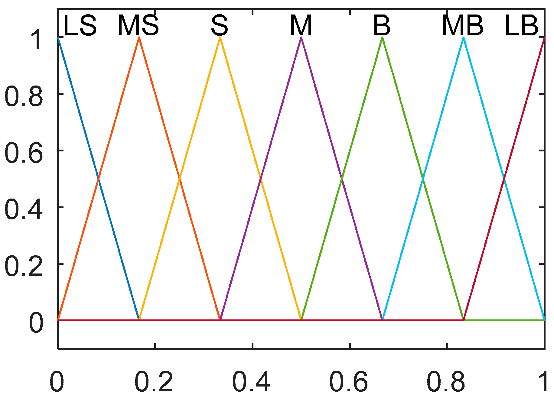
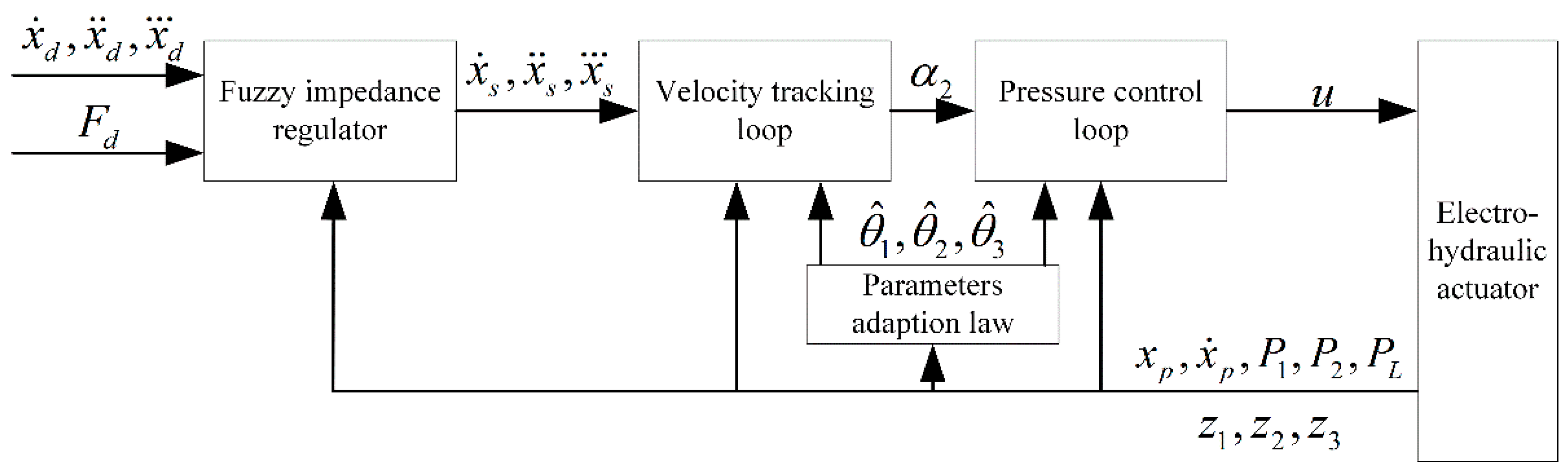
3. Fuzzy Impedance Control

From Figure 1, load force $F_L$ is positively correlated with the drive velocity, which should be kept in a regular range to protect the environment or workpieces. The desired dynamic relationship between velocity and force can be acquired through fuzzy impedance control. Define a first-order impedance rule

$$m_c{\ddot{e}}_x+b_c{\dot{e}}_x=e_F$$

(9)

where $m_c$ and $b_c$ are the desired mass and damping coefficient, respectively, $e_F=F_L-F_{Ld}$ is the force deviation, $F_{Ld}$ is the desired load force, ${\dot{e}}_x={\dot{x}}_d-\dot{x}$ is the velocity correction, and ${\ddot{e}}_x$ is its derivative.

A number of impedance rules are required to obtain a better dynamic relationship between velocity and force, due to the variation of velocity command and load force requirement. Therefore, fuzzy logic was adopted to adjust parameters of impedance rules. The parameters were predetermined based on the velocity command and load force requirement.

The fuzzy impedance controller was designed based on Mamdani-type fuzzy inference engine and center of gravity defuzzification. The input and output membership functions are defined as Figure 2 and Figure 3 respectively. Five membership functions are used for input variables $V_c$ and $F_c$, named as LS, S, M, B, LB in a range of [0, 1], whereas seven membership functions are used for output variables $M$ and $B$, named as LS, MS, S, M, B, MB, LB in a range of [0, 1]. The following are the scaling functions

$$\begin{array}{l}{V}_c=\frac{1}{2}+\frac{1}{v_{\max }-v_{\min }}\left(v_c-\frac{v_{\max }+v_{\min }}{2}\right)\\ F_c=\frac{1}{2}+\frac{1}{F_{Ln\max }-F_{Ln\min }}\left(F_{Ln}-\frac{F_{Ln\max }+F_{Ln\min }}{2}\right)\\ m_c=\left(m_{c\max }-m_{c\min }\right)\times M+m_{c\min }\\ b_c=\left(b_{c\max }-b_{c\min }\right)\times B+b_{c\min }\end{array}$$

(10)

where $v_c={\dot{x}}_d$ is the velocity command, $v_{\max }$ and $v_{\min }$ are its maximum and minimum values; $F_{Ln}$ is the nominal load force, and $F_{Ln\max }$ and $F_{Ln\min }$ are its maximum and minimum values. The nominal load force can be measured in advance. It is the force of the load cylinder when it moves at a desired velocity with a normal load. $m_{c\max }$ and $m_{c\min }$ are the maximum and minimum values of desired mass, and $b_{c\max }$ and $b_{c\min }$ are the maximum and minimum values of desired damping coefficient.

Table 1. Fuzzy rules of desired mass $M$.

$\mathit{M}$		${\mathit{V}}_{\mathit{c}}$
		LS	S	M	B	LB
$F_c$	LS	LB	LB	MB	B	M
	S	LB	MB	B	M	S
	M	MB	B	M	S	MS
	B	B	M	S	MS	LS
	LB	M	S	MS	LS	LS

and

Table 2. Fuzzy rules of desired damping coefficient $B$.

$\mathit{B}$		${\mathit{V}}_{\mathit{c}}$
		LS	S	M	B	LB
$F_c$	LS	LS	LS	MS	S	M
	S	LS	MS	S	M	B
	M	MS	S	M	B	MB
	B	S	M	B	MB	LB
	LB	M	B	MB	LB	LB

show the fuzzy rules, velocity command $V_c$ and nominal load force $F_c$ are the input variables, whereas desired mass $M$ and desired damping coefficient $B$ are the output variables. The goal of fuzzy impedance control is to adjust the load force to an acceptable range and provide an expected dynamic response between velocity and load force. According to the load cylinder in the system, a larger velocity leads to a larger load force that requires a smaller $m_c$ to improve the dynamics, and a larger $b_c$ to ease the restriction of the load force, respectively. A larger nominal load force also demands a smaller $m_c$ and a larger $b_c$, because the system is much more vulnerable to disturbances, which means a small change of velocity will result in a larger change of load force.

Considering fuzzy impedance control in the control process, the desired velocity trajectory turns into ${\dot{x}}_s={\dot{x}}_d-{\dot{\overline{e}}}_x$, and the derivatives become ${\ddot{x}}_s={\ddot{x}}_d-{\ddot{\overline{e}}}_x$, ${\stackrel{⃛}{x}}_s={\stackrel{⃛}{x}}_d-{\stackrel{⃛}{\overline{e}}}_x$. ${\dot{\overline{e}}}_x$, ${\ddot{\overline{e}}}_x$ and ${\stackrel{⃛}{\overline{e}}}_x$ are the computation results of (9), which are different from ${\dot{e}}_x$, ${\ddot{e}}_x$ and ${\stackrel{⃛}{e}}_x$.

Assumption 2.

Based on Assumption 1 and the first-order impedance rule,${\dot{x}}_s$, ${\ddot{x}}_s$, ${\stackrel{⃛}{x}}_s$are assumed to be bounded.

4. Adaptive Robust Velocity Control

4.1. Model Analysis

Parameter uncertainties are unavoidable in the electro-hydraulic system, such as the variations of $m$, $b$, $F_{fc}$, ${\beta }_e$, $k_q$, $k_x$ and so on. For simplicity, only the prime parameters, $m$, ${\beta }_e$ and $d_n$ (the nominal value of system uncertain nonlinearity $d$, $d=d_n+\tilde{d}$) are taken into parameters adaption.

Define the unknown parameters set as $\theta ={\left[\begin{array}{ccc}{\theta }_1& {\theta }_2& {\theta }_3\end{array}\right]}^T={\left[\begin{array}{ccc}1/m& d_n& {\beta }_e\end{array}\right]}^T$. Thus, the system dynamics (7) is transformed to

$$\left\{\begin{array}{l}{\dot{x}}_1=x_2\hfill \\ {\dot{x}}_2={\theta }_1\left[A_1{\overline{x}}_3-b{x}_2-F_L+G-F_{fc}\right]+{\theta }_2+\tilde{d}\hfill \\ {\dot{\overline{x}}}_3={\theta }_3\left[-f_1{x}_2-f_2{C}_t\left(x_3-x_4\right)+k_{qx}{f}_{3}u\right]\hfill \end{array}\right.$$

(11)

In practical applications, the extents of parameters and uncertain nonlinearity are known. So, we made the following assumption.

Assumption 3.

The parameter uncertainties and uncertain nonlinearity are bounded as

$$\begin{array}{l}\theta \in {\Omega }_{\theta }\triangleq \left\{\theta :{\theta }_{\min }\le \theta \le {\theta }_{\max }\right\}\hfill \\ \left|\tilde{d}\right|\le \delta \hfill \end{array}$$

(12)

In (12), the operation ‘$\le$’ is performed in terms of the corresponding elements of the vectors. In practice,${\theta }_{\min }={\left[\begin{array}{ccc}{\theta }_{1\min }& {\theta }_{2\min }& {\theta }_{3\min }\end{array}\right]}^T$, ${\theta }_{\max }={\left[\begin{array}{ccc}{\theta }_{1\max }& {\theta }_{2\max }& {\theta }_{3\max }\end{array}\right]}^T$, $\delta$are all known, and ${\theta }_{1\min }>0$, ${\theta }_{3\min }>0$.

4.2. Projection Mapping and Parameter Adaptation

Define $\widehat{\theta }$ as the estimation of $\theta$ and estimation error as $\tilde{\theta }=\theta -\widehat{\theta }$. A discontinuous projection [45] is defined as

$${\mathrm{Proj}}_{{\widehat{\theta }}_i}=\left\{\begin{array}{l}0, {\widehat{\theta }}_i={\theta }_{i\max } \mathrm{and} {•}_i>0\\ 0, {\widehat{\theta }}_i={\theta }_{i\min } \mathrm{and} {•}_i<0 \\ {•}_i,\mathrm{otherwise}\end{array}\right.$$

(13)

where $i=1,2,3$, ‘${•}_i$’ is the $i\mathrm{th}$ element of the vector ‘$•$’. Under this projection, an adaption law [45] is given

$$\dot{\widehat{\theta }}={\mathrm{Proj}}_{\widehat{\theta }}\left(\Gamma \tau \right), \mathrm{with} {\theta }_{\min }\le \widehat{\theta }\left(0\right)\le {\theta }_{\max }$$

(14)

where $\Gamma =diag\left\{\begin{array}{lll}{\Gamma }_1\hfill & {\Gamma }_2\hfill & {\Gamma }_3\hfill \end{array}\right\}$ is a symmetric positive definite adaption rate matrix, and $\tau$ is an adaption function to guarantee

$$\left\{\begin{array}{l}\widehat{\theta }\in {\Omega }_{\widehat{\theta }}\triangleq \left\{\widehat{\theta }:{\theta }_{\min }\le \widehat{\theta }\le {\theta }_{\max }\right\}\hfill \\ {\tilde{\theta }}^T\left[{\Gamma }^{-1}{\mathrm{Proj}}_{\widehat{\theta }}\left(\Gamma \tau \right)-\tau \right]\le 0\hfill \end{array}\right.$$

(15)

4.3. Velocity Control Design

The velocity control consists of an outer-loop velocity control and an inner-loop pressure control. According to the recursive backstepping technique, a velocity controller can be designed.

Step 1:

The velocity tracking error is defined as $z_1=x_2-{\dot{x}}_s$. Then, a sliding surface $z_2$ can be defined as

$$z_2=z_1+k_1{\displaystyle \int z_{1}dt}$$

(16)

where $k_1$ is a positive constant. Since making $z_1$ small or converge to zero is same as making $z_2$ small or converge to zero, the rest of the controller design concentrates on making $z_2$ as small as possible. Differentiating (16) and noting (11) based on Assumption 2, yielding

$${\dot{z}}_2={\theta }_1\left[A_1{\overline{x}}_3-b{x}_2-F_L+G-F_{fc}\right]+{\theta }_2+\tilde{d}-{\dot{x}}_{2eq}$$

(17)

where ${\dot{x}}_{2eq}={\ddot{x}}_s-k_1\left(x_2-{\dot{x}}_s\right)$.

A virtual control input ${\alpha }_2$ for ${\overline{x}}_3$ is designed as

$$\begin{array}{l}{\alpha }_2={\alpha }_{2a}+{\alpha }_{2s}\\ {\alpha }_{2a}=\frac{1}{A_1}\left[\left(b{x}_2+F_L-G+F_{fc}\right)+{\widehat{\theta }}_1\left({\dot{x}}_{2eq}-{\widehat{\theta }}_2\right)\right]\\ {\alpha }_{2s}={\alpha }_{2s1}+{\alpha }_{2s2}\\ {\alpha }_{2s1}=-k_{2s1}{z}_2, k_{2s1}\ge \frac{1}{{\theta }_{1\min }{A}_1}\left({‖C_{{\varphi }_2}\Gamma {\varphi }_2‖}^2+k_2\right)\\ {\tau }_2=w_2{\varphi }_2{z}_2, w_2>0\end{array}$$

(18)

where $C_{{\varphi }_2}$ is a positive definite constant diagonal matrix, and ${\alpha }_{2s2}$ is a robust control function, which will be designed later. $k_2$ and $w_2$ are positive constants, $k_{2s1}$ is the positive feedback coefficient in the outer velocity control loop. ${\varphi }_2$ is defined as

$${\varphi }_2={\left[\begin{array}{l}{A}_1{\alpha }_{2a}-b{x}_2-F_L+G-F_{fc}\hspace{1em}1\hspace{1em}0\hfill \end{array}\right]}^T$$

(19)

${\alpha }_{2a}$ is a model compensation through online parameter adaption, ${\alpha }_{2s}$ is a robust control law, of which ${\alpha }_{2s2}$ is a function satisfying the following conditions [45]

$$\begin{array}{l}\mathrm{i} z_2\left[{\theta }_1{\alpha }_{2s2}-{\tilde{\theta }}^T{\varphi }_2+\tilde{d}\right]\le {\epsilon }_2\\ \mathrm{ii} z_2{\alpha }_{2s2}\le 0\end{array}$$

(20)

where ${\epsilon }_2$ is a positive constant that can arbitrarily be small.

Define a following Lyapunov function

$$V_2=\frac{1}{2}{w}_2{z}_2^2$$

(21)

Let $z_3={\overline{x}}_3-{\alpha }_2$ represent the tracking error of the inner pressure control loop, and taking (17)–(19) into account, the time derivative of $V_2$ is expressed as

$${\dot{V}}_2=w_2{\theta }_1{A}_1{z}_2{z}_3+w_2{A}_1{z}_2\left({\theta }_1{\alpha }_{2s2}-\tilde{\theta }{\varphi }_2+\tilde{d}\right)-w_2{\theta }_1{A}_1{k}_{2s1}{z}_2^2$$

(22)

Step 2:

The time derivative of $z_3$ is expressed as

$${\dot{z}}_3={\theta }_3\left[-f_1{x}_2-f_2{C}_t\left(x_3-x_4\right)+k_{qx}{f}_{3}u\right]-{\dot{\alpha }}_{2c}-{\dot{\alpha }}_{2u}$$

(23)

where

$$\begin{array}{l}{\dot{\alpha }}_{2c}=\frac{\partial {\alpha }_2}{\partial x_1}{x}_2+\frac{\partial {\alpha }_2}{\partial x_2}{\widehat{\dot{x}}}_2+\frac{\partial {\alpha }_2}{\partial t}\\ {\dot{\alpha }}_{2u}=\frac{\partial {\alpha }_2}{\partial x_2}\left[-\left(A_1{\overline{x}}_3-b{x}_2-F_L+G-F_{fc}\right){\tilde{\theta }}_1-{\tilde{\theta }}_2+\tilde{d}\right]+\frac{\partial {\alpha }_2}{\partial \widehat{\theta }}\dot{\widehat{\theta }}\end{array}$$

(24)

${\dot{\alpha }}_{2c}$ is the calculable part of ${\alpha }_2$, which will be used in the control function design, ${\dot{\alpha }}_{2u}$ is the incalculable part which should be handled with robust feedback. ${\widehat{\dot{x}}}_2$ represents the calculable part of ${\dot{x}}_2$, from (11), ${\widehat{\dot{x}}}_2$ can be expressed as

$${\widehat{\dot{x}}}_2={\widehat{\theta }}_1\left[A_1{\overline{x}}_3-b{x}_2-F_L+G-F_{fc}\right]+{\widehat{\theta }}_2$$

(25)

The actual control input $u$ needs to be designed to make ${\overline{x}}_3$ track the virtual control input ${\alpha }_2$. Similar as Step 1, $u$ is given by

$$\begin{array}{l}u=u_a+u_s\\ u_a=\frac{1}{k_{qx}{f}_3}\left[f_1{x}_2+f_2{C}_t\left(x_3-x_4\right)+\frac{{\dot{\alpha }}_{2c}}{{\widehat{\theta }}_3}-\frac{w_2{\widehat{\theta }}_1{A}_1{z}_2}{w_3{\widehat{\theta }}_3}-\frac{\partial {\alpha }_2}{\partial \widehat{\theta }}{\mathrm{Proj}}_{\widehat{\theta }}\left(\Gamma \tau \right)\right]\\ u_s=u_{s1}+u_{s2}\\ u_{s1}=-\frac{k_{3s1}}{k_{qx}{f}_3}{z}_3,k_{3s1}\ge \frac{1}{{\theta }_{3\min }}\left(k_3+{‖\frac{\partial {\alpha }_2}{\partial \widehat{\theta }}{C}_{{\theta }_3}‖}^2+{‖C_{{\varphi }_3}\Gamma {\varphi }_3‖}^2\right)\\ \tau ={\tau }_2+w_3{\varphi }_3{z}_3, w_3>0\end{array}$$

(26)

where $C_{{\theta }_3}$ and $C_{{\varphi }_3}$ are positive definite constant diagonal matrixes, and ${\alpha }_{2s2}$ is a robust control function designed later. $k_3$ and $w_3$ are positive constants, $k_{3s1}$ is the positive feedback coefficient in the inner pressure control loop. ${\varphi }_3$ is defined as

$${\varphi }_3=\left[\begin{array}{c}\frac{w_2}{w_3}{A}_1{z}_2-\frac{\partial {\alpha }_2}{\partial x_2}\left(A_1{\overline{x}}_3-b{x}_2-F_L+G-F_{fc}\right)\\ -\frac{\partial {\alpha }_2}{\partial x_2}\\ k_{qx}{f}_3{u}_a-f_1{x}_2-f_2{C}_t\left(x_3-x_4\right)\end{array}\right]$$

(27)

$u_a$ is a model compensation through online parameter adaption, $u_s$ is a robust control law, of which $u_{s2}$ is a function satisfying the following conditions [45]

$$\begin{array}{l}\mathrm{i} z_3\left[{\theta }_3{k}_{qx}{f}_3{u}_{s2}-{\tilde{\theta }}^T{\varphi }_3-\frac{\partial {\alpha }_2}{\partial x_2}\tilde{d}\right]\le {\epsilon }_3\\ \mathrm{ii} z_3{u}_{s2}\le 0\end{array}$$

(28)

where ${\epsilon }_3$ is a positive constant which can arbitrarily be small.

Define a following Lyapunov function

$$V_3=V_2+\frac{1}{2}{w}_3{z}_3^2$$

(29)

Taking Equations (22)–(24) and (26) into account, the time derivative of $V_3$ is expressed as

$$\begin{array}{ll}{\dot{V}}_3=& w_2{A}_1{z}_2\left({\theta }_1{\alpha }_{2s2}-\tilde{\theta }{\varphi }_2+\tilde{d}\right)-w_2{\theta }_1{A}_1{k}_{2s1}{z}_2^2\\ & +w_3{z}_3\left[{\theta }_3{k}_{qx}{f}_3{u}_{s2}-{\tilde{\theta }}^T{\varphi }_3-\frac{\partial {\alpha }_2}{\partial x_2}\tilde{d}\right]-w_3{\theta }_3{k}_{3s1}{z}_3^2-w_3{z}_3\frac{\partial {\alpha }_2}{\partial \widehat{\theta }}\dot{\widehat{\theta }}\end{array}$$

(30)

4.4. Stability of ARC

For simplicity, choosing nonlinear controller gains $k_{2s1}$ and $k_{3s1}$ large enough [45] so that the inequality conditions in (18) and (26) are satisfied for $C_{{\theta }_j}=diag\left\{c_{{\theta }_{jl}}\right\},l=1,2,3,j=3$ and $C_{{\varphi }_k}=diag\left\{c_{{\varphi }_{kl}}\right\},k=2,3$ with $c_{{\varphi }_{kl}}^2\ge \frac{3w_k{w}_3}{4c_{{\theta }_{3l}}^2},\forall k,l$, then the control input as (26) with the adaption law (14) guarantees that

$$V_4\le \exp \left(-{\lambda }_{V}t\right)V_4\left(0\right)+\frac{{\epsilon }_V}{{\lambda }_V}\left[1-\exp \left(-{\lambda }_{V}t\right)\right]$$

(31)

where ${\lambda }_V=2\min \left\{k_2,k_3\right\}$ and ${\epsilon }_V=A_1{w}_2{\epsilon }_2+w_3{\epsilon }_3$.

Proof of (31).

$$\begin{array}{l}\left|w_3{z}_3\frac{\partial {\alpha }_2}{\partial \widehat{\theta }}\dot{\widehat{\theta }}\right|=\left|{\sum }_{k=2}^3{w}_3{z}_3\frac{\partial {\alpha }_2}{\partial \widehat{\theta }}\frac{1}{\sqrt{3w_3}}{C}_{{\theta }_3}\sqrt{3w_3}{C}_{{\theta }_3}^{-1}\Gamma {\varphi }_k{w}_k{z}_k\right|\\ \le {\sum }_{k=2}^3\left(\frac{1}{\sqrt{3}}\sqrt{w_3}\left|z_3\right|‖C_{{\theta }_3}{\left(\frac{\partial {\alpha }_2}{\partial \widehat{\theta }}\right)}^T‖\right)\left(\sqrt{3w_3{w}_k}‖C_{{\theta }_3}^{-1}\Gamma {\varphi }_k‖\sqrt{w_k}\left|z_k\right|\right)\\ \le {\sum }_{k=2}^3\left[\frac{1}{3}{w}_3{z}_3^2{‖C_{{\theta }_3}{\left(\frac{\partial {\alpha }_2}{\partial \widehat{\theta }}\right)}^T‖}^2+\frac{3}{4}{w}_3{w}_k{‖C_{{\theta }_3}^{-1}\Gamma {\varphi }_k‖}^2{w}_k{z}_k^2\right]\\ \le w_3{‖C_{{\theta }_3}{\left(\frac{\partial {\alpha }_2}{\partial \widehat{\theta }}\right)}^T‖}^2{z}_3^2+{\sum }_{k=2}^3{w}_k\left(\frac{3}{4}{w}_k{w}_3{‖C_{{\theta }_3}^{-1}\Gamma {\varphi }_k‖}^2\right)z_k^2\end{array}$$

(32)

If $C_{{\varphi }_j}$ and $C_{{\theta }_j}$ satisfy the aforementioned condition, then (32) becomes

$$\left|w_3{z}_3\frac{\partial {\alpha }_2}{\partial \widehat{\theta }}\dot{\widehat{\theta }}\right|\le w_3{‖C_{{\theta }_3}{\left(\frac{\partial {\alpha }_2}{\partial \widehat{\theta }}\right)}^T‖}^2{z}_3^2+{\sum }_{k=2}^3{w}_k\left({‖C_{{\theta }_3}\Gamma {\varphi }_k‖}^2\right)z_k^2$$

(33)

Thus, considering the formula for $k_{2s1}$ and $k_{3s1}$, (30) turns into

$$\begin{array}{ll}{\dot{V}}_3\le & -w_2{k}_2{z}_2^2-w_3{k}_3{z}_3^2+w_2{A}_1{z}_2\left({\theta }_1{\alpha }_{2s2}-\tilde{\theta }{\varphi }_2+\tilde{d}\right)\\ & +w_3{z}_3\left[{\theta }_3{k}_{qx}{f}_3{u}_{s2}-{\tilde{\theta }}^T{\varphi }_3-\frac{\partial {\alpha }_2}{\partial x_2}\tilde{d}\right]\end{array}$$

(34)

Noting the condition i of Equations (20) and (28) yields

$${\dot{V}}_3\le -w_2{k}_2{z}_2^2-w_3{k}_3{z}_3^2+A_1{w}_2{\epsilon }_2+w_3{\epsilon }_3\le -2{\lambda }_V{V}_3+{\epsilon }_V$$

(35)

which leads to (31).

If, after a finite time, $t_0$, $\tilde{d}=0$, i.e., only exiting parameter uncertainties, apart from results in (31), asymptotic output tracking (i.e., zero final tracking error) can be achieved [45].

This can be proved by defining a new Lyapunov function

$$V=V_3+\frac{1}{2}{\tilde{\theta }}^T{\Gamma }^{-1}\tilde{\theta }$$

(36)

Assume the unknown parameter vector is constant; thus, $\dot{\tilde{\theta }}=\dot{\widehat{\theta }}$, so the time derivative of $V$ is

$$\dot{V}\le -{\sum }_{j=2}^3{w}_j{k}_j{z}_j^2-{\tilde{\theta }}^T\tau +{\tilde{\theta }}^T{\Gamma }^{-1}\dot{\widehat{\theta }}\le -{\sum }_{j=2}^3{w}_j{k}_j{z}_j^2$$

(37)

Therefore, the stability of the ARC designed above is proved. □

5. Stability Analysis of the Whole System

As Figure 4 shown, a fuzzy impedance controller and a nonlinear velocity controller are synthesized together in the whole cascade system. The parameters of impedance rules are predetermined. Thus, the impedance system (9) is a time invariant first-order system with positive coefficients. According to the concerned load system, the input $e_F$ is bounded. Therefore, the impedance system is stable based on Routh’s stability criterion.

Defining a sliding function as

$$s_I=m_c{\ddot{e}}_x+b_c{\dot{e}}_x-e_F$$

(38)

it can be seen that the sliding function (38) generates the expected impedance behavior (46), when $s_I$ vanishes [46]. The above definitions yield

$$\begin{array}{ll}{s}_I& =m_c\left({\ddot{x}}_d-\ddot{x}\right)+b_c\left({\dot{x}}_d-\dot{x}\right)-e_F\\ & =m_c\left(-{\dot{z}}_1+{\ddot{\overline{e}}}_x\right)+b_c\left(-z_1+{\dot{\overline{e}}}_x\right)-e_F\\ & =-\left(m_c{\dot{z}}_1+b_c{z}_1\right)\end{array}$$

(39)

Since the stability of ARC is already proved, $z_1$ will converge to zero after a finite time only under parameter uncertainties. To make the force vary smoothly, the response of ARC is designed much faster than the fuzzy impedance controller. Thus, ${\ddot{x}}_s$ and ${\dot{x}}_2$ can be finally treated as small enough, since ${\dot{x}}_d$ is always set as constant and the load is assumed to vary slowly in practice. Then, ${\dot{z}}_1={\dot{x}}_2-{\ddot{x}}_s$ can be considered small enough to make $s_I$ converge to zero. Consequently, impedance performance can be guaranteed under certain conditions.

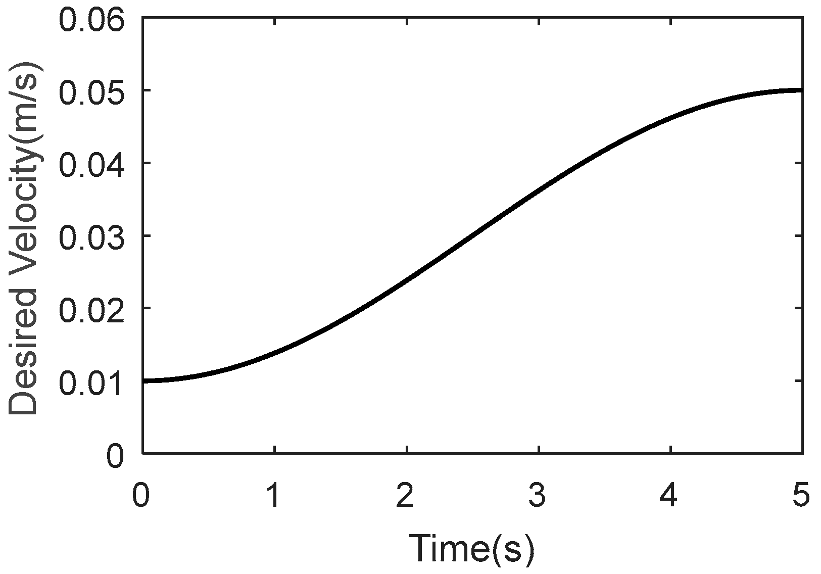
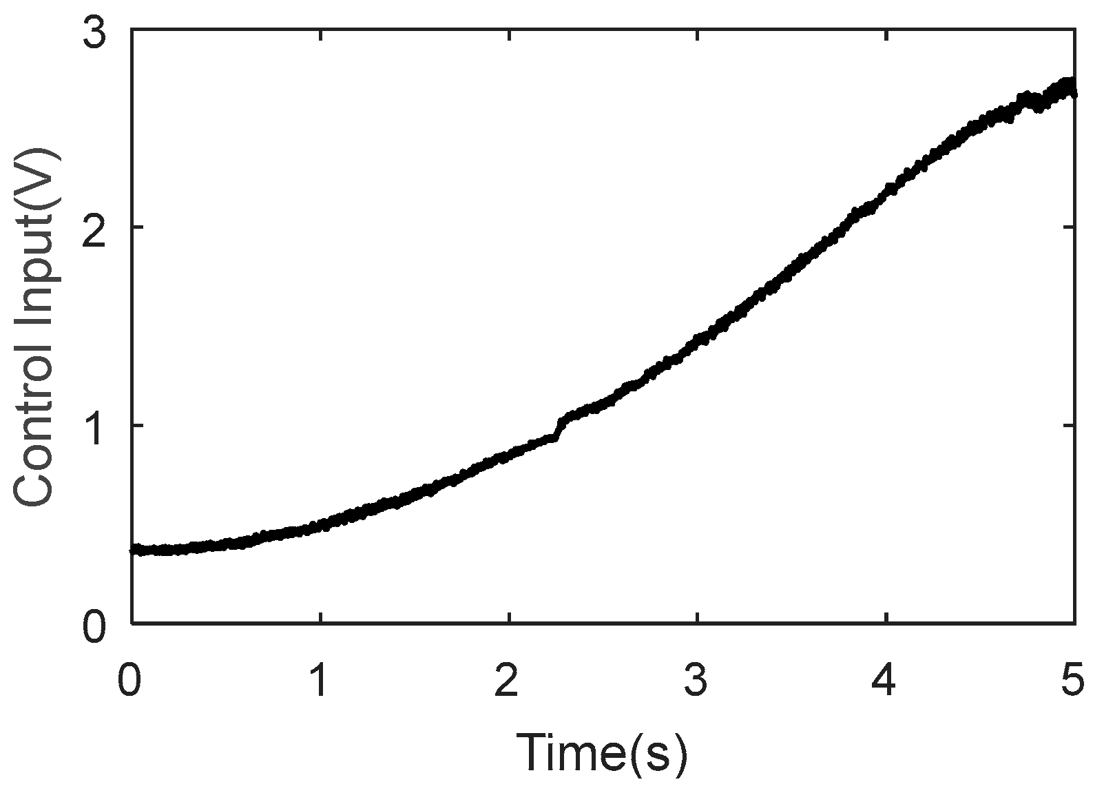
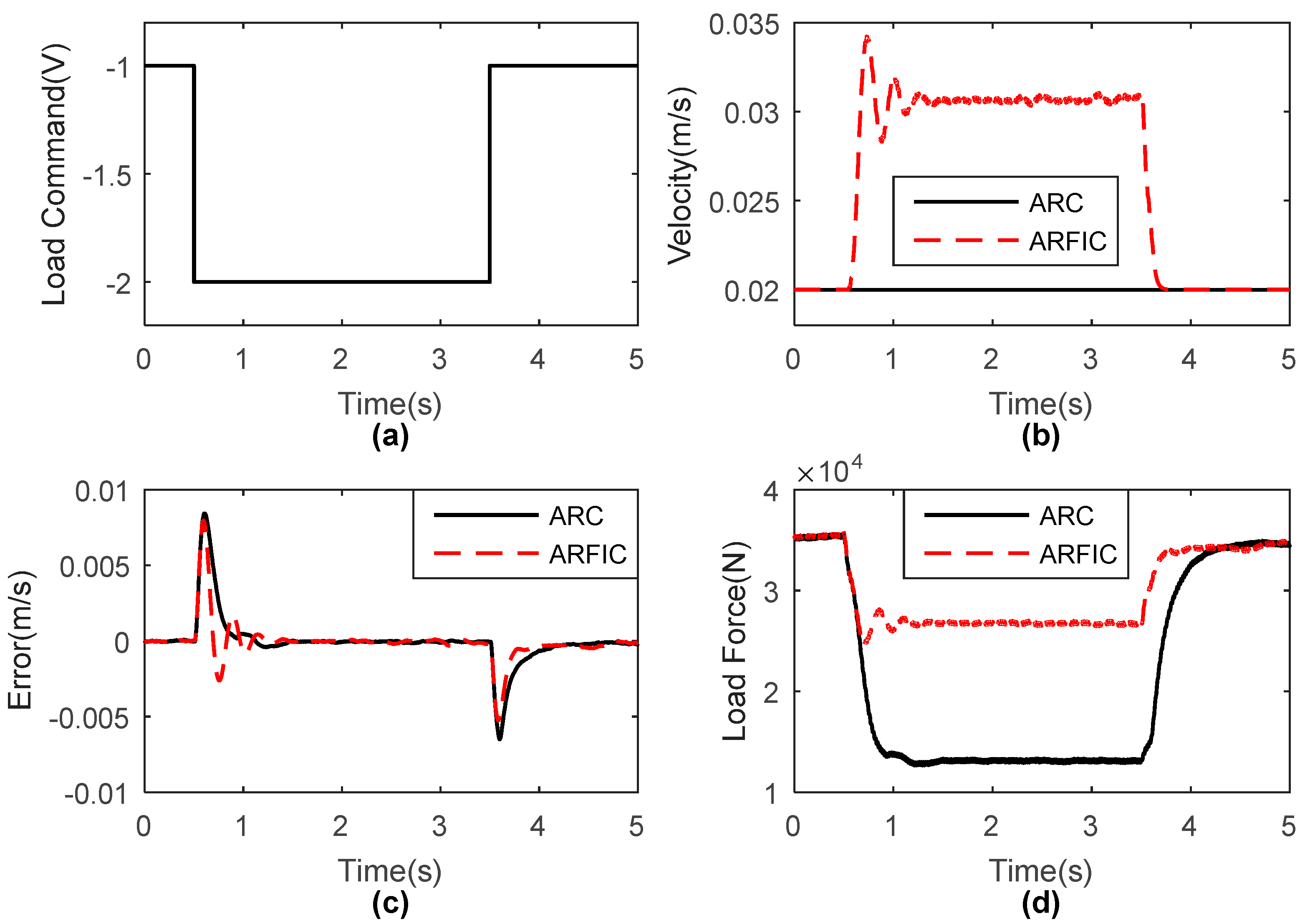
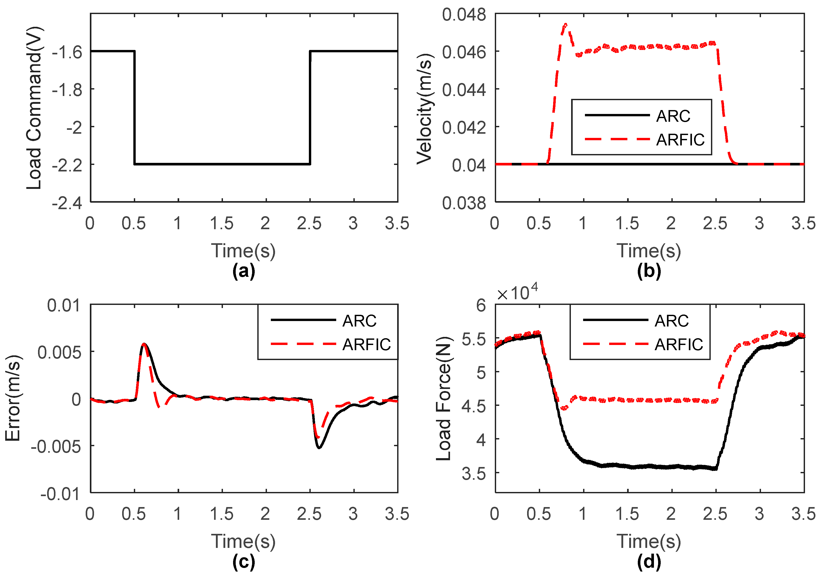
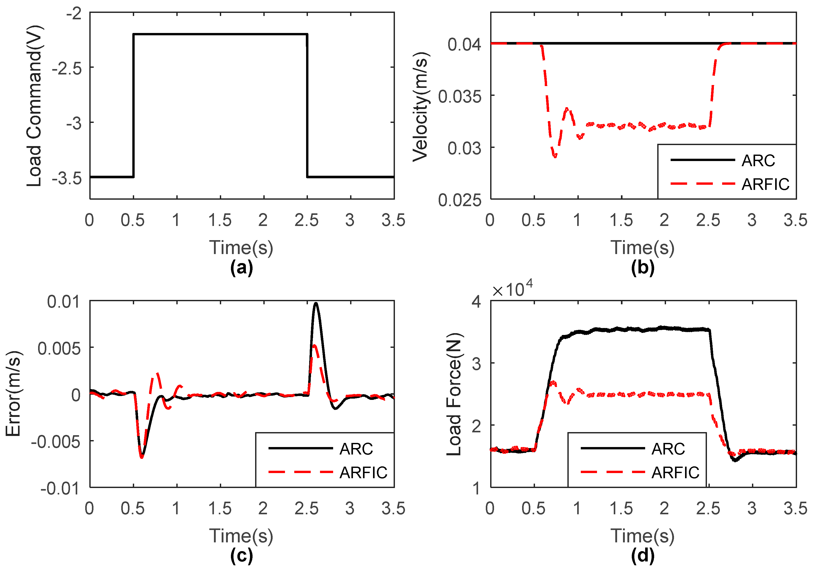
6. Experimental Results

Experiments were conducted to validate the performance of the proposed ARFIC. The drive cylinder and the load cylinder were both controlled by servo valves. Four pressure sensors were utilized. A position sensor was used to obtain the displacement and velocity of the drive cylinder. A data acquisition card was employed to collect data and output control inputs. The control strategy was implemented in the MATLAB Simulink Realtime environment with a 1 kHz control rate.

Firstly, ARC (without impedance control) was tested.

Table 3. Parameters of the electro-hydraulic system.

Symbol	Value	Unit
$A_1$	$5.0265\times {10}^{-3}$	${\mathrm{m}}^2$
$A_2$	$3.0631\times {10}^{-3}$	${\mathrm{m}}^2$
$b$	$1\times {10}^5$	$\mathrm{Ns}/\mathrm{m}$
$F_{fc0}$	$1.2\times {10}^3$	$\mathrm{N}$
$\eta$	$10$
$G$	$1715$	$\mathrm{N}$
$A_3$	$3.8485\times {10}^{-3}$	${\mathrm{m}}^2$
$P_s$	$2.1\times {10}^6$	$\mathrm{Pa}$
$P_t$	$0$	$\mathrm{Pa}$
$C_t$	$0$	${\mathrm{m}}^4/\mathrm{kg}$
$k_{qx}$	$3.5635\times {10}^{-8}$	${\mathrm{m}}^3/\left(\mathrm{sV}\sqrt{\mathrm{Pa}}\right)$

lists the parameters of the electro-hydraulic system.

Table 4. Nominal Values and bounds of ${\theta }_i$.

Symbol (Unit)	Nominal Value	${\mathit{\theta }}_{\mathit{i}\mathbf{m}\mathbf{i}\mathbf{n}}$	${\mathit{\theta }}_{\mathit{i}\mathbf{m}\mathbf{a}\mathbf{x}}$
${\theta }_1$$(1/\mathrm{kg}$)	$5.7143\times {10}^{-3}$	$5\times {10}^{-4}$	$6\times {10}^{-2}$
${\theta }_2$$(\mathrm{N}/\mathrm{kg}$)	$0$	$-30$	$30$
${\theta }_3$$(\mathrm{Pa}$)	$7\times {10}^8$	$7\times {10}^7$	$7\times {10}^9$

and

Table 5. Parameters of ARC.

Symbol	Value	Symbol	Value
$k_1$	$56$	${\Gamma }_1$	$1\times {10}^{-18}$
$k_{2s1}$	$1.86\times {10}^7$	${\Gamma }_2$	$5\times {10}^{-12}$
$k_{3s1}$	$5\times {10}^{-7}$	${\Gamma }_3$	$1\times {10}^4$

list controller parameters. Figure 5 shows the desired velocity trajectory, ${\dot{x}}_d=0.02\sin \left(\frac{\pi }{5}t+\frac{3\pi }{2}\right)+0.03 \mathrm{m}/\mathrm{s}$. $u_L=-2 \mathrm{V}$ is the servo valve command of load cylinder. As Figure 6 shown, the tracking errors of ARC were small. Figure 7 shows the control input and Figure 8 shows the parameter estimations. ARC achieved accurate velocity tracking, because the parameter uncertainties and uncertain nonlinearities could be compensated. The initial values of parameter estimations were defined according to parameter identification when ${\dot{x}}_d=0.02 \mathrm{m}/\mathrm{s}$. However, it cannot be guaranteed that parameter estimations converged to true values because only control errors were used to drive the parameter adaption law, and persistent excitation condition [47] may not be satisfied.

Next, ARFIC was verified when the velocity command was constant at 0.02 m/s and 0.04 m/s. The parameters of the fuzzy impedance rule were chosen according to

Table 6. Parameters of the fuzzy impedance rule.

Symbol	Value	Unit
$v_{\max }$	$0.05$	$\mathrm{m}/\mathrm{s}$
$v_{\min }$	$0.01$	$\mathrm{m}/\mathrm{s}$
$F_{Ln\max }$	$6\times {10}^4$	$\mathrm{N}$
$F_{Ln\min }$	$2000$	$\mathrm{N}$
$m_{c\max }$	$850$	${\mathrm{Ns}}^2/\mathrm{m}$
$m_{c\min }$	$350$	${\mathrm{Ns}}^2/\mathrm{m}$
$b_{c\max }$	$1\times {10}^6$	$\mathrm{Ns}/\mathrm{m}$
$b_{c\min }$	$1\times {10}^5$	$\mathrm{Ns}/\mathrm{m}$

. ARFIC was tested compared with ARC (without impedance control), to validate the effectiveness of fuzzy impedance control. A step-like signal was applied to the servo valve which controls the load cylinder. A pressure sensor was used to measure the load force in experiments.

As shown in Figure 9a, the velocity command was 0.02 m/s, and the load command changed in a step-wise manner from $-1 \mathrm{V}$ to $-0.7 \mathrm{V}$ then to $-1 \mathrm{V}$. The regulated velocity commands are shown in Figure 9b, which guaranteed an expected impedance behavior when load command change occurred. A smooth smaller velocity command was produced by fuzzy impedance control in ARFIC. The load force of ARFIC was kept in a close range, as shown in Figure 9d. Tracking errors with respect to unregulated or regulated velocity command are shown in Figure 9c. Both ARFIC and ARC achieved accurate velocity tracking. ARFIC showed a great ability to handle load change through velocity adjustment.

Fuzzy impedance control worked when the deviation of load force exceeded 10% of the nominal value in experiments. It can be seen that dynamic balance behavior was achieved with a fuzzy logic-based impedance control. To validate the effectiveness of ARFIC further, some other load and velocity commands were tested. Similarly, in all kinds of cases, ARFIC demonstrated accurate velocity tracking and impedance regulation between velocity and force. The experiment results are shown in Figure 10, Figure 11 and Figure 12. A smooth regulated velocity command was generated when the load force was beyond the regular range. ARFIC could keep the load force in a close range, comparing with ARC.

Impedance control regulates the load force in a close area which can protect the environment or workpieces. It is quite useful in practice, because motion control has to consider the contact force with the environment or workpieces. ARFIC provides a solution to keep a compromise of velocity control and force control. In ARFIC, contact force is considered as the protection for the system, which should be kept in an acceptable range. Accurate velocity tracking can be achieved, when the contact force is in the regular range, but the velocity command is adjusted, when the contact force exceeds the regular range.

7. Conclusions

In this research, an adaptive robust controller and an impedance control strategy were developed to handle both velocity and force control for an electro-hydraulic actuator. The developed control strategy has the merits of an adaptive robust controller and impedance controller. Parameter uncertainties and uncertain nonlinearities could be compensated through ARC, which led to high-accuracy velocity tracking. A compromise of velocity control and force control could be acquired through the impedance controller. Fuzzy logic was employed to tune the parameters of the impedance controller to obtain better performance. The velocity command was regulated by the fuzzy impedance controller, which is the control target of ARC. The stability of the whole cascade system was analyzed. In experiments, parameter uncertainties and uncertain nonlinearities were successfully canceled, and high-accuracy velocity tracking and force regulation were also attained, which validated the effectiveness of the ARFIC strategy.

References

1. Sha, D.; Bajic, V.B.; Yang, H. New model and sliding mode control of hydraulic elevator velocity tracking system. Simulat. Pract. Theory 2002, 9, 365–385. [Google Scholar] [CrossRef]
2. Yang, H.; Yang, J.; Xu, B. Computational simulation and experimental research on speed control of VVVF hydraulic elevator. Control Eng. Pract. 2004, 12, 563–568. [Google Scholar]
3. Nam, Y.; Hong, S.K. Force control system design for aerodynamic load simulator. Control Eng. Pract. 2002, 10, 549–558. [Google Scholar] [CrossRef]
4. Truong, D.Q.; Ahn, K.K. Force control for hydraulic load simulator using self-tuning grey predictor—Fuzzy PID. Mechatronics 2009, 19, 233–246. [Google Scholar] [CrossRef]
5. Sirouspour, M.R.; Salcudean, S.E. Nonlinear control of hydraulic robots. IEEE Trans. Rob. Autom. 2001, 17, 173–182. [Google Scholar] [CrossRef]
6. Zhu, W.-H.; Piedboeuf, J.-C. Adaptive Output Force Tracking Control of Hydraulic Cylinders with Applications to Robot Manipulators. J. Dyn. Syst. Meas. Control 2005, 127, 206. [Google Scholar] [CrossRef]
7. Guo, K.; Pan, Y.; Yu, H. Composite Learning Robot Control with Friction Compensation: A Neural Network-Based Approach. IEEE Trans. Ind. Electron. 2019, 66, 7841–7851. [Google Scholar] [CrossRef]
8. Guo, K.; Pan, Y.; Zheng, D.; Yu, H. Composite learning control of robotic systems: A least squares modulated approach. Automatica 2020, 111, 108612. [Google Scholar] [CrossRef]
9. Farivarnejad, H.; Moosavian, S.A.A. Multiple Impedance Control for object manipulation by a dual arm underwater vehicle–manipulator system. Ocean. Eng. 2014, 89, 82–98. [Google Scholar] [CrossRef]
10. Wang, T.; Li, Y.; Zhang, J.; Zhang, Y. A novel bilateral impedance controls for underwater tele-operation systems. Appl. Soft Comput. 2020, 91, 106194. [Google Scholar] [CrossRef]
11. Wang, Q.; Xie, X.; Shahrour, I.; Huang, Y. Use of deep learning, denoising technic and cross-correlation analysis for the prediction of the shield machine slurry pressure in mixed ground conditions. Autom. Constr. 2021, 128, 103741. [Google Scholar] [CrossRef]
12. Zhang, H.; Fang, J.; Yu, H.; Hu, H.; Yang, Y. Disturbance observer-based adaptive position control for a cutterhead anti-torque system. PLoS ONE 2022, 17, e0268897. [Google Scholar] [CrossRef] [PubMed]
13. Hogan, N. Impedance control: An approach to manipulation: Part I—Theory. J. Dyn. Syst. Meas. Control 1985, 107, 1–7. [Google Scholar] [CrossRef]
14. Hogan, N. Impedance control: An approach to manipulation: Part II—Implementation. J. Dyn. Syst. Meas. Control 1985, 107, 8–16. [Google Scholar] [CrossRef]
15. Hogan, N. Impedance Control: An Approach to Manipulation: Part III—Applications. J. Dyn. Syst. Meas. Control 1985, 107, 17–24. [Google Scholar] [CrossRef]
16. Jamwal, P.K.; Hussain, S.; Ghayesh, M.H.; Rogozina, S.V. Impedance Control of an Intrinsically Compliant Parallel Ankle Rehabilitation Robot. IEEE Trans. Ind. Electron. 2016, 63, 3638–3647. [Google Scholar] [CrossRef]
17. Hyun, D.J.; Seok, S.; Lee, J.; Kim, S. High speed trot-running: Implementation of a hierarchical controller using proprioceptive impedance control on the MIT Cheetah. Int. J. Robot Res. 2014, 33, 1417–1445. [Google Scholar] [CrossRef]
18. Zhang, J.; Liu, W.; Gao, L.E.; Li, L.; Li, Z. The master adaptive impedance control and slave adaptive neural network control in underwater manipulator uncertainty teleoperation. Ocean. Eng. 2018, 165, 465–479. [Google Scholar] [CrossRef]
19. Michel, Y.; Rahal, R.; Pacchierotti, C.; Giordano, P.R.; Lee, D. Bilateral Teleoperation With Adaptive Impedance Control for Contact Tasks. IEEE Robot. Autom. Lett. 2021, 6, 5429–5436. [Google Scholar] [CrossRef]
20. Hu, H.; Cao, J. Adaptive variable impedance control of dual-arm robots for slabstone installation. ISA Trans. 2022, 128, 397–408. [Google Scholar] [CrossRef]
21. Zhao, X.; Han, S.; Tao, B.; Yin, Z.; Ding, H. Model-Based Actor–Critic Learning of Robotic Impedance Control in Complex Interactive Environment. IEEE Trans. Ind. Electron. 2022, 69, 13225–13235. [Google Scholar] [CrossRef]
22. Plummer, A.R. Feedback linearization for acceleration control of electrohydraulic actuators. Proc. Inst. Mech. Eng. Part I J. Syst. Contr. Eng. 2005, 211, 395–406. [Google Scholar] [CrossRef]
23. Daher, N.; Ivantysynova, M. An Indirect Adaptive Velocity Controller for a Novel Steer-by-Wire System. J. Dyn. Syst. Meas. Control. Trans. ASME 2014, 136, 051012. [Google Scholar] [CrossRef]
24. Ahn, K.K.; Nam, D.N.C.; Jin, M. Adaptive Backstepping Control of an Electrohydraulic Actuator. IEEE/ASME Trans. Mech. 2014, 19, 987–995. [Google Scholar] [CrossRef]
25. Zhu, D. Sliding mode synchronous control for fixture clamps system driven by hydraulic servo systems. Proc. Inst. Mech. Eng. C J. Mec. 2007, 221, 1039–1045. [Google Scholar]
26. Lin, Y.; Shi, Y.; Burton, R. Modeling and robust discrete-time sliding-mode control design for a fluid power electrohydraulic actuator (EHA) system. IEEE/ASME Trans. Mech. 2013, 18, 1–10. [Google Scholar] [CrossRef]
27. Yao, B.; Tomizuka, M. Adaptive robust control of SISO nonlinear systems in a semi-strict feedback form. Automatica 1997, 33, 893–900. [Google Scholar] [CrossRef]
28. Yao, B.; Bu, F.P.; Reedy, J.; Chiu, G.T.C. Adaptive robust motion control of single-rod hydraulic actuators: Theory and experiments. IEEE/ASME Trans. Mech. 2000, 5, 79–91. [Google Scholar]
29. Chen, Z.; Yao, B.; Wang, Q.F. Accurate Motion Control of Linear Motors With Adaptive Robust Compensation of Nonlinear Electromagnetic Field Effect. IEEE/ASME Trans. Mech. 2013, 18, 1122–1129. [Google Scholar] [CrossRef]
30. Zhang, Q.; Fang, J.H.; Wei, J.H.; Xiong, Y.; Wang, G. Adaptive robust motion control of a fast forging hydraulic press considering the nonlinear uncertain accumulator model. Proc. Inst. Mech. Eng. Part I J. Syst. Contr. Eng. 2016, 230, 483–497. [Google Scholar] [CrossRef]
31. Chen, S.; Chen, Z.; Yao, B.; Zhu, X.; Zhu, S.; Wang, Q.; Song, Y. Adaptive robust cascade force control of 1-DOF hydraulic exoskeleton for human performance augmentation. IEEE/ASME Trans. Mech. 2017, 22, 589–600. [Google Scholar] [CrossRef]
32. Chen, W.H. Disturbance observer based control for nonlinear systems. IEEE/ASME Trans. Mech. 2004, 9, 706–710. [Google Scholar] [CrossRef]
33. Guo, K.; Wei, J.H.; Fang, J.H.; Feng, R.L.; Wang, X.C. Position tracking control of electro-hydraulic single-rod actuator based on an extended disturbance observer. Mechatronics 2015, 27, 47–56. [Google Scholar] [CrossRef]
34. Li, S.Z.; Wei, J.H.; Guo, K.; Zhu, W.L. Nonlinear Robust Prediction Control of Hybrid Active-Passive Heave Compensator with Extended Disturbance Observer. IEEE Trans. Ind. Electron. 2017, 64, 6684–6694. [Google Scholar] [CrossRef]
35. Wei, J.; Zhang, Q.; Li, M.; Shi, W. High-performance motion control of the hydraulic press based on an extended fuzzy disturbance observer. Proc. Inst. Mech. Eng. Part I J. Syst. Contr. Eng. 2016, 230, 1044–1061. [Google Scholar] [CrossRef]
36. Zhang, Q.; Wei, J.; Fang, J.; Li, M. Nonlinear motion control of the hydraulic press based on an extended piecewise disturbance observer. Proc. Inst. Mech. Eng. Part I J. Syst. Contr. Eng. 2016, 230, 830–850. [Google Scholar] [CrossRef]
37. Shi, W.; Wei, J.; Fang, J.; Li, M. Nonlinear cascade control of high-response proportional solenoid valve based on an extended disturbance observer. Proc. Inst. Mech. Eng. Part I J. Syst. Contr. Eng. 2018, 233, 921–934. [Google Scholar] [CrossRef]
38. Li, M.; Shi, W.; Wei, J.; Fang, J.; Guo, K.; Zhang, Q. Parallel Velocity Control of an Electro-Hydraulic Actuator with Dual Disturbance Observers. IEEE Access 2019, 7, 56631–56641. [Google Scholar] [CrossRef]
39. Wang, L.-X. A Course in Fuzzy Systems and Control; Prentice Hall: Englewood Cliffs, NJ, USA, 1996. [Google Scholar]
40. Ho, T.H.; Ahn, K.K. Speed control of a hydraulic pressure coupling drive using an adaptive fuzzy sliding-mode control. IEEE/ASME Trans. Mech. 2012, 17, 976–986. [Google Scholar] [CrossRef]
41. Tian, Q.Y.; Wei, J.H.; Fang, J.H.; Guo, K. Adaptive fuzzy integral sliding mode velocity control for the cutting system of a trench cutter. Front. Inform. Technol. Electron. Eng. 2016, 17, 55–66. [Google Scholar] [CrossRef]
42. Shibata, M.; Murakami, T.; Ohnishi, K. A unified approach to position and force control by fuzzy logic. IEEE Trans. Ind. Electron. 1996, 43, 81–87. [Google Scholar] [CrossRef]
43. Xu, Z.-L.; Fang, G. Fuzzy-Neural Impedance Control for Robots. In Robotic Welding, Intelligence and Automation; Tarn, T.-J., Zhou, C., Chen, S.-B., Eds.; Springer: Berlin/Heidelberg, Germany, 2004; pp. 263–275. [Google Scholar]
44. Fateh, M.M.; Alavi, S.S. Impedance control of an active suspension system. Mechatronics 2009, 19, 134–140. [Google Scholar] [CrossRef]
45. Yao, B.; Bu, F.P.; Chiu, G.T.C. Non-linear adaptive robust control of electro-hydraulic systems driven by double-rod actuators. Int. J. Control 2001, 74, 761–775. [Google Scholar] [CrossRef]
46. Xu, Q. Robust impedance control of a compliant microgripper for high-speed position/force regulation. IEEE Trans. Ind. Electron. 2015, 62, 1201–1209. [Google Scholar] [CrossRef]
47. Slotine, J.-J.E.; Li, W. Applied Nonlinear Control; Prentice Hall: Englewood Cliffs, NJ, USA, 1991. [Google Scholar]
Figure 1. Schematic diagram of the electro-hydraulic system.
Applsci 12 09575 g001
Figure 2. Membership functions for inputs.
Applsci 12 09575 g002
Figure 3. Membership functions for outputs.
Applsci 12 09575 g003
Figure 4. Schematic diagram of the proposed ARFIC control strategy.
Applsci 12 09575 g004
Figure 5. Desired velocity trajectory.
Applsci 12 09575 g005
Figure 6. Tracking errors of ARC.
Applsci 12 09575 g006
Figure 7. Control input of ARC.
Applsci 12 09575 g007
Figure 8. Parameter estimations of ARC: (a) estimation of θ 1 ; (b) estimation of θ 2 ; (c) estimation of θ 3 .
Applsci 12 09575 g008
Figure 9. Tracking performance with a 0.02 m/s velocity command and 1   V 0.7   V 1   V load command: (a) load command; (b) velocity commands; (c) velocity tracking errors; (d) load forces.
Applsci 12 09575 g009
Figure 10. Tracking performance with a 0.02 m/s velocity command and 1   V 2   V 1   V load command: (a) load command; (b) velocity commands; (c) velocity tracking errors; (d) load forces.
Applsci 12 09575 g010
Figure 11. Tracking performance with a 0.04 m/s velocity command and 1.6   V 2.2   V 1.6   V load command: (a) load command; (b) velocity commands; (c) velocity tracking errors; (d) load forces.
Applsci 12 09575 g011
Figure 12. Tracking performance with a 0.04 m/s velocity command and 3 . 5   V 2.2   V 3.5   V load command: (a) load command; (b) velocity commands; (c) velocity tracking errors; (d) load forces.
Applsci 12 09575 g012