One Novel Dynamic-Load Time-Domain-Identification Method Based on Function Principle

Abstract

In order to ensure the reliability of the structural design, it is necessary to know the external loads acting on the structure. In this paper, we propose a novel method to identify the dynamic loads based on function principles in the time domain. Assuming the external load remains constant within one micro segment, we establish a linear relationship between external load and structural response in the micro segments based on the mechanical energy conservation law. Next, the external load is obtained by solving the inverse problem in each micro-segment. Finally, the external load in the whole time domain is achieved by fitting the load-identification results in each micro segment. In order to verify the effectiveness and accuracy, single-force and two-force identification, and load identification with noise simulations, are performed on the structures, and the identification results are compared to the ones of the traditional time-domain method with a deviation of less than 5%. The proposed method can effectively solve the problem of cumulative errors in the time-domain method, while its resistance to noise interference is also strong. At last, we verify the experimental performance of the proposed method. The experimental results show the effectiveness and high accuracy of the proposed method. This work presents a first attempt to solve the structural dynamic load with an approach based on a function principle.

1. Introduction

In engineering practice, in order to study the dynamic characteristics of the structure, carry out structural parameter design and failure analysis, and ensure the reliability of the structure, it is often necessary to accurately know the external load acting on the structure [1]. However, in most cases, due to the constraints of the surrounding environment and technical conditions, the dynamic load on the structure is usually difficult to directly measure, but the dynamic response is relatively easy to measure, so it is proposed to measure the dynamic response of the structure (displacement, velocity, and acceleration) to identify the load [2,3].

Dynamic load identification can be divided into the frequency domain method [4,5,6] and the time domain method [7,8,9,10]. The frequency domain method for dynamic-load identification is the process of establishing the frequency response function matrix of the system in the frequency domain and identifying the dynamic input through the output of the system. Compared with the frequency domain identification method, the time domain method started relatively late. H. Ory, H. Glaser, and D. Holzdepp first proposed the time domain method for dynamic-load identification when analyzing the rocket loading [11]. The time-domain rule of dynamic-load identification is to use the parameters of the structure to establish a reverse model of the structural system in the time domain, to solve the input dynamic load based on the output response data. In the past few decades, many researchers have proposed some mature time domain methods for load identification. M. L. Wang, T. Kreitinger, and H. L. Luo proposed the SWAT (weighted acceleration method) method in the time domain [12]. The SWAT method can identify steady-state load and impact load, but it is only suitable for structures with rigid-body modes and the resultant force of dynamic loads is sought, so its application has great limitations [13,14]. The wavelet deconvolution method has the characteristics of multi-resolution analysis and time-frequency analysis, so this method has advantages in terms of the signal reconstruction of the impact load [15]. Moreover, the wavelet deconvolution method has strong anti-noise ability and improves the accuracy of load identification [16]. The generalized Chebyshev orthogonal polynomial is used to fit the modal load function, combined with the Duhamel integral equation to identify the modal load of the system, and then the dynamic load is solved by modal coordinate transformation [17,18,19]. This method cannot identify harmonic loads containing white noise. In addition, because the recursive chain calculation format is used in the load-identification process, it is prone to error accumulation [20,21,22].

In the existing load-identification time-domain method, due to the accumulated error in time, the accuracy of the identification result will be reduced or even lead to the divergence of the identified load. Therefore, in this paper, we propose a novel time domain method for dynamic-load identification based on the conservation of mechanical energy. The collected time domain signal is divided into several isochronous micro-segments, and the load is identified for each micro-segment. It is equivalent to every micro-element segment being a new beginning, and the identified results are different from each other. This eliminates errors caused by time accumulation and greatly improve the accuracy of dynamic-load identification in the time domain. This method is a new attempt to reconstruct the structural dynamic load by the relationship between the work done by external forces and the structural energy.

This paper aims to identify the unknown dynamic load acting on structures based on the functional principle method. The remainder of this paper is organized as follows. The energy conservation principle of the single degree freedom system and multi-degree freedom system are presented in Section 2. The simulation calculation is explained in Section 3, while in Section 4 the experiments are run to evaluate the accuracy and the efficiency of the proposed method. We finish with some concluding remarks in Section 5.

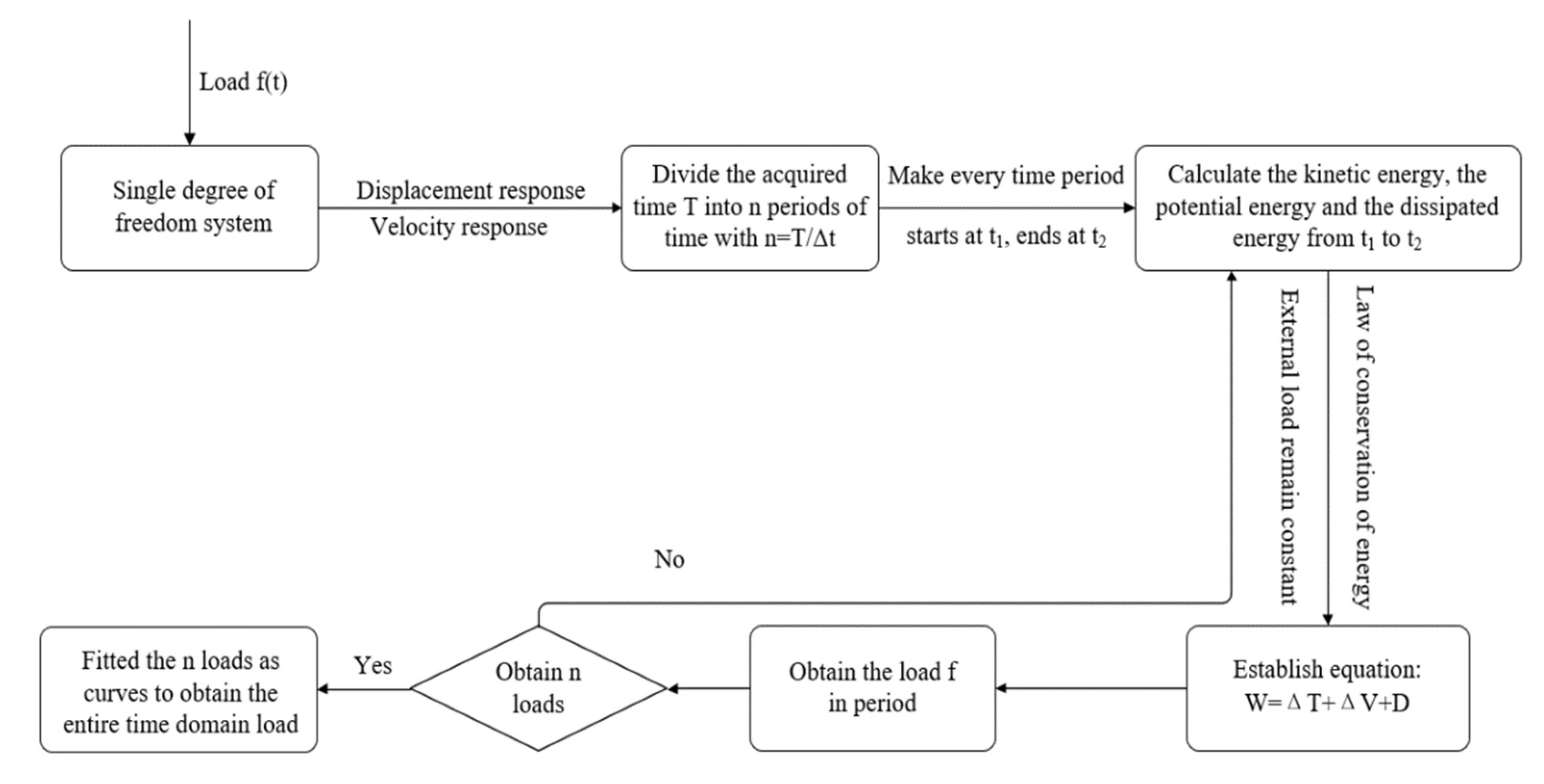
2. Function Principle Dynamic Load Identification Method

According to the law of conservation of energy, the work done by the external force to the system equals the variation of the energy of the system, which includes kinetic energy, potential energy, and dissipation energy.

In the multiple-degree-of-freedom vibration system, from t₁ to t₂, the work done by the external force to the system equals the sum of the variation of the kinetic energy, the potential energy, and the dissipated energy of the system, which is written as [23]

$$W=\mathrm{\Delta }T+\mathrm{\Delta }V+D$$

(1)

where $W,\mathrm{\Delta }T,\mathrm{\Delta }V$, and D refer to, respectively, the work done by the external force, the variation of the kinetic energy, the variation of the potential energy, and the dissipated energy generated by the damp in this period.

The work done by the external force to the system is [23]

$$W={{\displaystyle {\int }_{t_1}^{t_2}f\left(t\right)dx\left(t\right)}}^{ }$$

(2)

where $f\left(t\right) \mathrm{and} x\left(t\right)$ represent the external force and the displacement.

The expressions of the kinetic energy and the potential energy are [23]

$$T=\frac{1}{2}m{\dot{u}}^2$$

(3)

$$\mathrm{V}=\frac{1}{2}k\mathrm{\Delta }{u}^2$$

(4)

The expression of the dissipated energy is [23]

$$D={\displaystyle {\int }_{t_1}^{t_2}c{\dot{u}}^{2}dt}$$

(5)

where $\dot{u}$ represents the velocity of the certain mass and ∆u represents a certain spring deformation.

Suppose in a tiny period of time, the magnitude of external force f remain constant, donated as $\overline{f}$; then, the work done by the external forces in this segment is

$$W=\overline{f}\mathrm{\Delta }u$$

(6)

where ∆u represents the displacement of external load application point.

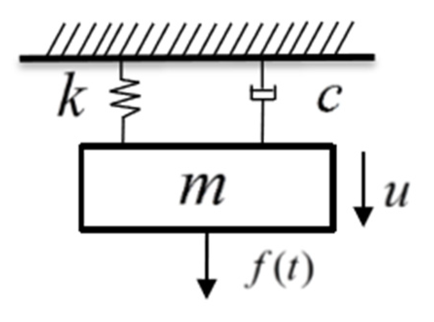
2.1. Time-Domain Identification Method of Dynamic Load Based on Function Principle for Single-Degree-of-Freedom System

Figure 1 presents a single-degree-of-freedom system, in which the mass is represented by m and the spring stiffness is noted K. The external force acting on the system is unknown, and the displacement and velocity of the system can be measured.

Assuming a zero initial state and the system is in equilibrium position, the entire duration of the observation is T, and divided into n tiny periods with the interval time ∆t, then $n=T/\mathrm{\Delta }t$. In one period of the time that starts at t₁ and ends at t₂, the variation of the energy of the system is

$$\mathrm{\Delta }E=\frac{1}{2}m\dot{u}{\left(t_2\right)}^2+\frac{1}{2}ku{\left(t_2\right)}^2-[\frac{1}{2}m\dot{u}{\left(t_1\right)}^2+\frac{1}{2}ku{\left(t_1\right)}^2]+{\displaystyle {\int }_{t_1}^{t_2}c{\dot{u}}^{2}dt}$$

(7)

where $u \mathrm{and} \dot{u}$ represent the displacement and velocity of the mass block, respectively.

During this short period, because the external load changes continuously and the amount of change is small, the external load remains constant. Then, the external force in this short period is

$$W=\overline{f}\mathrm{\Delta }u$$

(8)

$$\mathrm{\Delta }u=u\left(t_2\right)-u\left(t_1\right)$$

(9)

According to the law of conservation of energy, we can obtain the equation

$$W=\mathrm{\Delta }E$$

(10)

The equation has only one unknown number $\overline{f}$, so the external load on the micro segment can be obtained

$$\overline{f}=\frac{\frac{1}{2}m\dot{u}{\left(t_2\right)}^2+\frac{1}{2}ku{\left(t_2\right)}^2-[\frac{1}{2}m\dot{u}{\left(t_1\right)}^2+\frac{1}{2}ku{\left(t_1\right)}^2]+{\displaystyle {\int }_{t_1}^{t_2}c{\dot{u}}^{2}dt}}{u\left(t_2\right)-u\left(t_1\right)}$$

(11)

Similarly, apply the above method on each micro-period of time to obtain the external load value of each micro segment. Fit all the obtained external loads to a curve to obtain the external load value in the entire time domain.

The flow chart of load identification for the single-degree-of-freedom system is shown as Figure 2.

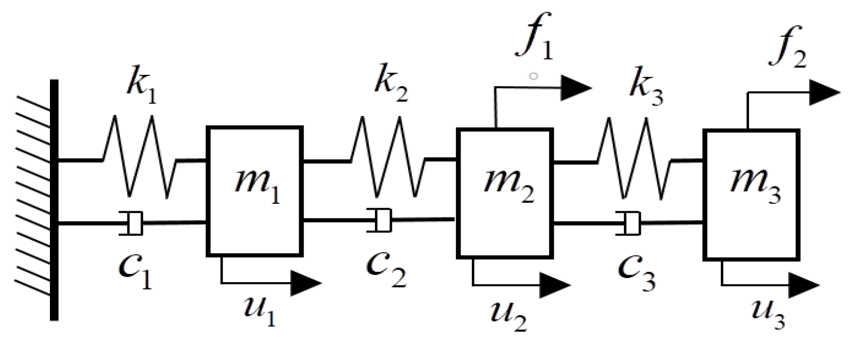
2.2. Time-Domain Identification Method of Multi-Point Dynamic Loads Based on Function Principle for Multiple-Degree-of-Freedom System

For multi-point loads acting on a multiple-degree-of-freedom system, we take the two external loads of the three-degrees-of-freedom system shown in Figure 3 as an example and apply external loads on the mass m₂ and m₃.

In this system, the kinetic energy is the sum of the kinetic energy of each degree, while the potential energy and the dissipated energy of the damping include the relative displacement quantity and the relative velocity quantity. Taking a three-degrees-of-freedom system as an example, the expressions of the kinetic energy, the potential energy, and the dissipated energy are as follows:

The expression of kinetic energy

$$T={\displaystyle \sum _{i=1}^3\frac{1}{2}}{m}_i{u}_i^2$$

(12)

The expression of potential energy

$$V=\frac{1}{2}{k}_1{u}_1^2+\frac{1}{2}{k}_2{\left(u_2-u_1\right)}^2+\frac{1}{2}{k}_3{\left(u_3-u_2\right)}^2$$

(13)

The expression of dissipated energy

$$D={\int }_{t_1}^{t_2}[c_1{\dot{u}}_1^2+c_2{\left({\dot{u}}_2-{\dot{u}}_1\right)}^2+c_3{\left({\dot{u}}_3-{\dot{u}}_2\right)}^2]dt$$

(14)

The acquisition time domain T is divided into n micro segments by Δt; if there are m external loads that need to be identified, then m segments regarded as an identification unit.

Take the system shown in the Figure 3 as an example, in which there are two external loads to be identified, which are applied on the mass m₂ and m₃; then, there are two segments $\left(t_1-t_2,t_2-t_3\right)$ in an identification unit.

In the first segments of an identification unit t₁ to t₂, the external loads are regarded as constant ${\overline{f}}_1$ and ${\overline{f}}_2$, and the displacements of the mass are Δu₁ and Δu₂, respectively. Based on the relationship between work done by the external load and the change of energy, the following equation can be listed:

$${\overline{f}}_1\mathrm{\Delta }{u}_2+{\overline{f}}_2\mathrm{\Delta }{u}_3=\mathrm{\Delta }T+\mathrm{\Delta }V+D=W$$

(15)

where the variation of kinetic energy ΔT, the variation of potential energy ΔV, and the dissipated energy D from t₁ to t₂ are given as

$$\mathrm{\Delta }T={\displaystyle \sum _{i=1}^3\frac{1}{2}}{m}_i{\dot{u}}_i{\left(t_2\right)}^2-{\displaystyle \sum _{i=1}^3\frac{1}{2}}{m}_i{\dot{u}}_i{\left(t_1\right)}^2$$

(16)

$$\begin{array}{cc}\mathrm{\Delta }V& =\frac{1}{2}\left\{k_1{u}_1{\left(t_2\right)}^2+k_2{\left[u_2\left(t_2\right)-u_1\left(t_2\right)\right]}^2+k_3{\left[u_3\left(t_2\right)-u_2\left(t_2\right)\right]}^2\right\}\\ & -\frac{1}{2}\left\{k_1{u}_1{\left(t_1\right)}^2+k_2{\left[u_2\left(t_1\right)-u_1\left(t_1\right)\right]}^2+k_3{\left[u_3\left(t_1\right)-u_2\left(t_1\right)\right]}^2\right\}\end{array}$$

(17)

$$D={\int }_{t_1}^{t_2}[c_1{\dot{u}}_1^2+c_2{\left({\dot{u}}_2-{\dot{u}}_1\right)}^2+c_3{\left({\dot{u}}_3-{\dot{u}}_2\right)}^2]dt$$

(18)

In another segment, from t₂ to t₃, based on the function principle, we can obtain the equation about ${\overline{f}}_1$ and ${\overline{f}}_2$.

$${\overline{f}}_1\mathrm{\Delta }{u^{\prime }}_2+{\overline{f}}_2\mathrm{\Delta }{u^{\prime }}_3=\mathrm{\Delta }{T}^{\prime }+\mathrm{\Delta }{V}^{\prime }+D^{\prime }=W^{\prime }$$

(19)

Simultaneously, we can obtain Equations (15) and (19),

$$\left[\begin{array}{c}{\overline{f}}_1\\ {\overline{f}}_2\end{array}\right]\left[\begin{array}{cc}\mathrm{\Delta }{u}_2& \mathrm{\Delta }{u}_3\\ \mathrm{\Delta }{u^{\prime }}_2& \mathrm{\Delta }{u^{\prime }}_3\end{array}\right]=\left[\begin{array}{c}W\\ W^{\prime }\end{array}\right]$$

(20)

By solving Equation (20), we can obtain the external load values ${\overline{f}}_1$ and ${\overline{f}}_2$ in an identification unit

$$\left[\begin{array}{c}{\overline{f}}_1\\ {\overline{f}}_2\end{array}\right]=\left[\begin{array}{c}W\\ W^{\prime }\end{array}\right]{\left[\begin{array}{cc}\mathrm{\Delta }{u}_2& \mathrm{\Delta }{u}_3\\ \mathrm{\Delta }{u^{\prime }}_2& \mathrm{\Delta }{u^{\prime }}_3\end{array}\right]}^{-1}$$

(21)

The flow chart of multi-load identification of the multiple-degree-of-freedom system is as shown in Figure 4:

3. Simulation Example

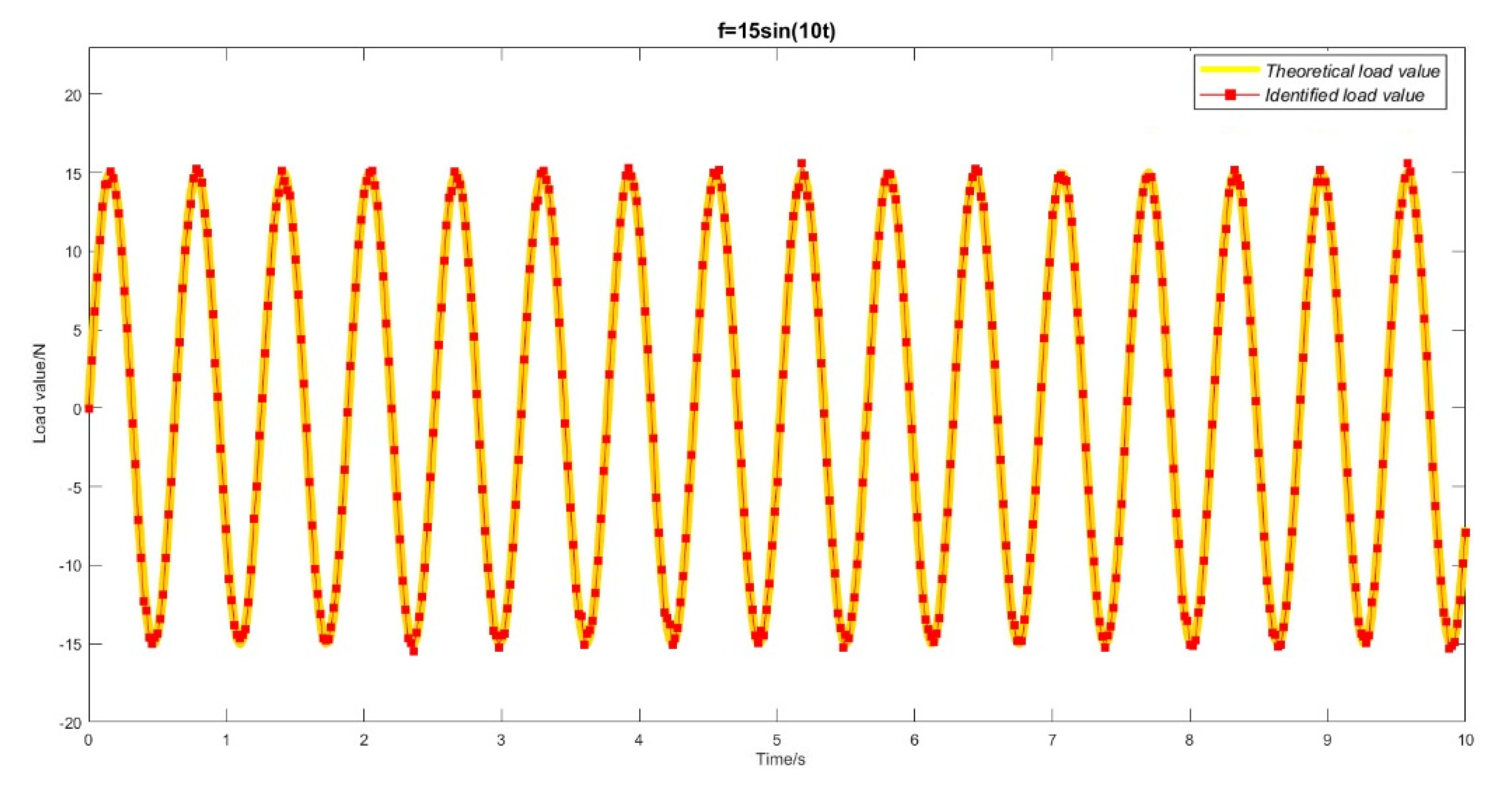
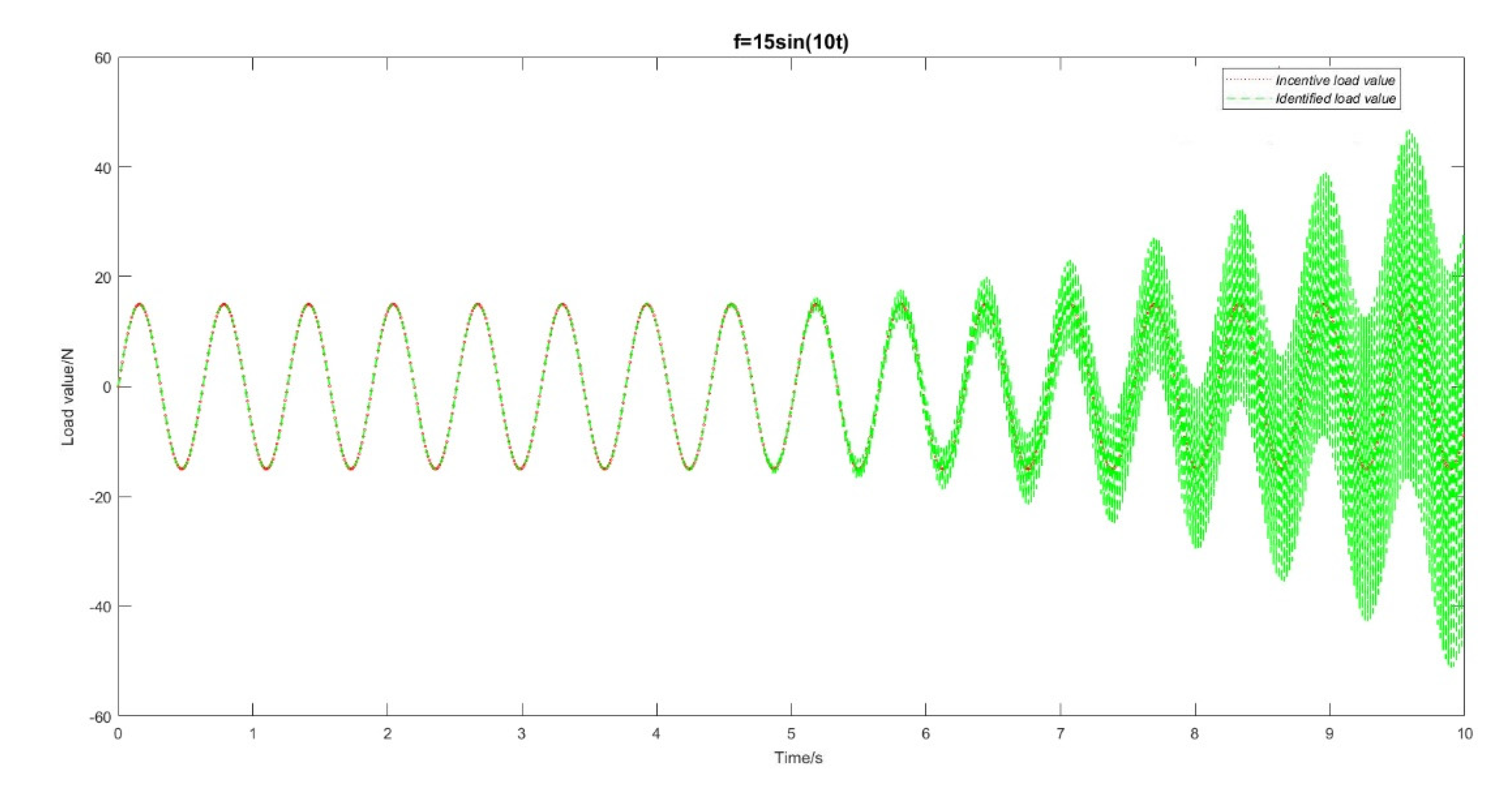
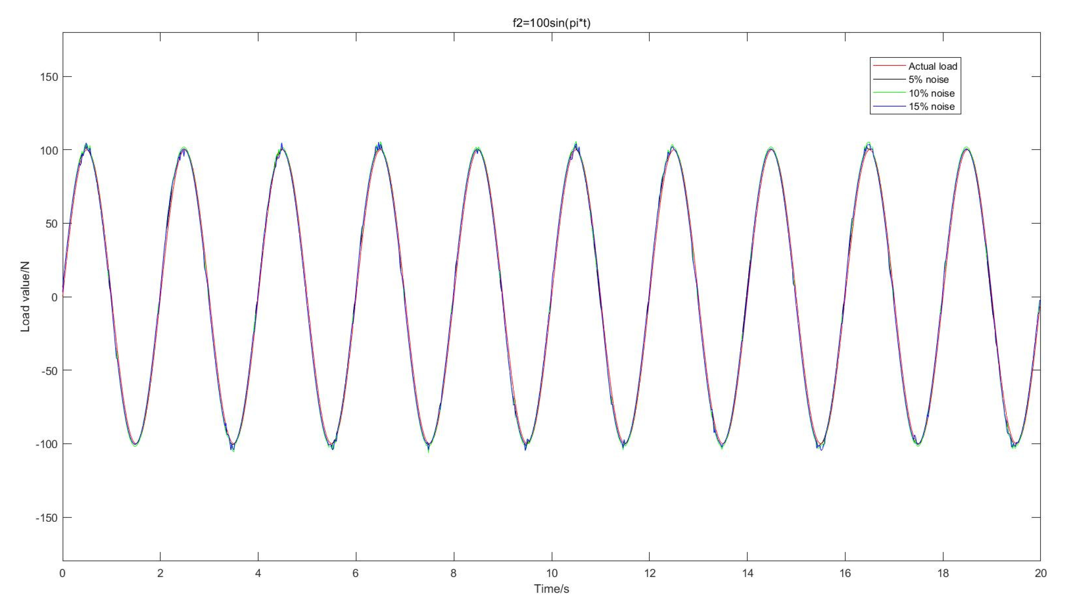
3.1. Example 1: Single-Degree-of-Freedom System

Here, we take the single-degree-of-freedom system as an example as shown in Figure 1. We put an external force $f=15\sin (10t)$ on the system. The time interval between t₁ and t₂ is $\mathrm{\Delta }t=0.02 \mathrm{s}$. We set $m=2 \mathrm{kg}$, $k=20 \mathrm{N}/\mathrm{m}$, and $c=0.05$. The initial state is 0, and observation lasts for 10 s. The identification results are as follows.

From the Figure 5, we can see that the load identified by the algorithm is highly consistent with the real load applied to the system, with a deviation of less than 5%. The feasibility of this method for the load identification of the single-degree-of-freedom system is proven. There is no divergence of the results caused by accumulated errors in the time domain. Using the Newmark method [24] for load identification in the same load-identification model, the identification results are as follows.

Figure 6 indicates that the load identified by the Newmark method has good identification accuracy in the first 5 s and then starts to diverge; the error exceeds 100% after 8 s. However, there are no corresponding problems in the function principle identification method; the load identification of each micro segment is independent of the others, and there is no accumulated error.

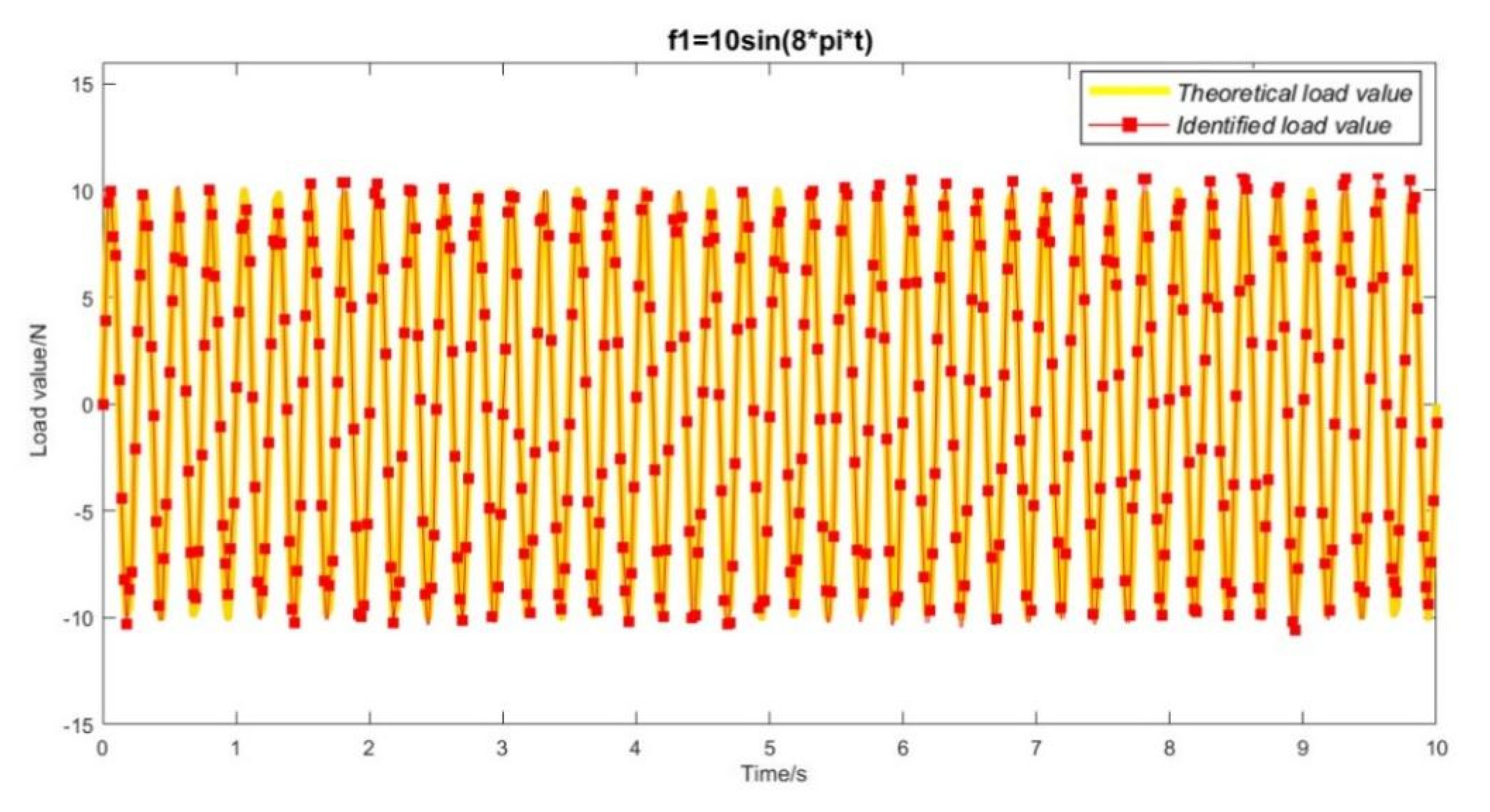
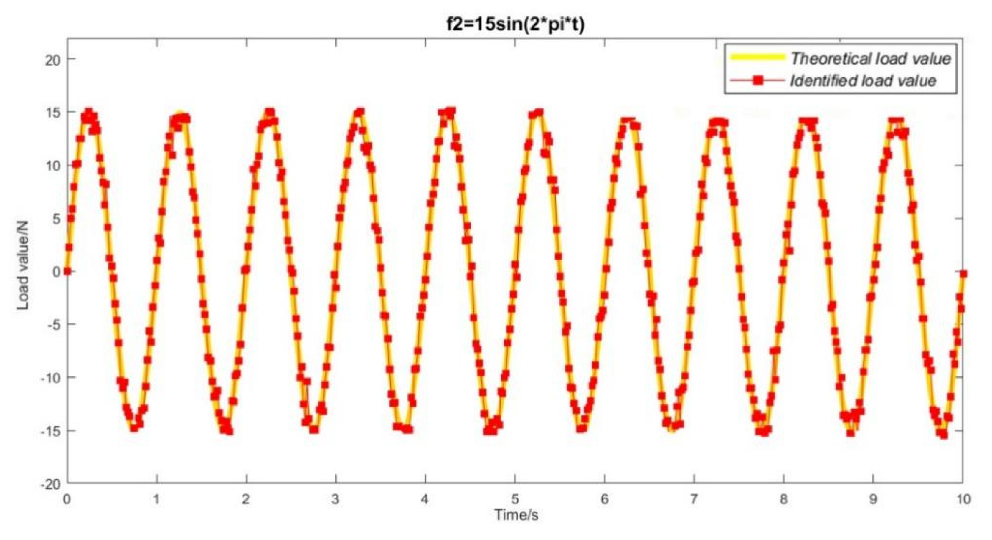
3.2. Multiple-Degree-of-Freedom System

Case 1: In this example, we take the multiple-degree-of-freedom system shown in Figure 3 as a research object and identify the dynamic load on it. We set the stiffness of the system to $k_1=4 \mathrm{N}/\mathrm{m},k_2=5 \mathrm{N}/\mathrm{m}$ and $k_3=6 \mathrm{N}/\mathrm{m}$, the mass to $m_1=3 \mathrm{kg},m_2=2 \mathrm{kg},m_3=1 \mathrm{kg}$, and the damping to $c=0.01$. Apply the external load $f=8\cos \left(t\right)\sin \left(3t\right)$ on the mass m₃. The external force represents a kind of relatively complex force, whose amplitude changes harmoniously. The similar performance is also able to be obtained for other functions. The time interval from t₁ to t₂ is $\mathrm{\Delta }t=0.02 \mathrm{s}$. The initial state is 0, and observation lasts for 10 s. The identification results are as follows.

Figure 7 presents that the load identified by the algorithm is highly consistent with the actual load applied to the system, with a deviation of less than 5%, which proves the feasibility of the method for the load identification of multiple-degree-of-freedom systems.

The previous example verifies the feasibility of the method for identifying a single load of a multiple-degree-of-freedom system. Next, we will use another example to discuss the feasibility of identifying a multiple-degree-of-freedom system under multiple loads. Let us also take the three-degrees-of-freedom system shown in Figure 3 as an example.

Case 2: Assume that the stiffness of the system is $k_1=4 \mathrm{N}/\mathrm{m},k_2=5 \mathrm{N}/\mathrm{m},k_3=6 \mathrm{N}/\mathrm{m}$; the mass is $m_1=3 \mathrm{kg},m_2=2 \mathrm{kg},m_3=4 \mathrm{kg}$; and the damping is $c=0.01$. The forces applied on mass m₂ and m₃ are $f_1=10\sin \left(8\pi t\right)$ and $f_2=15\sin \left(2\pi t\right)$, respectively. The time interval from t₁ to t₂ is $\mathrm{\Delta }t=0.02 \mathrm{s}$. The initial state is 0, and observation lasts for 10 s. The identification results are as follows.

From the identification results of two loading points of three degrees of freedom identified in Figure 8 and Figure 9, each excitation is identified with a derivation less than 5%, which proves the feasibility of the method for multi-loads identification of multiple-degree-of-freedom system.

Case 3: Assume that the system parameters are the same as in Case 2. the loads applied on the mass m₂ and m₃ are $f_1=50\sin (2\pi t)$ and $f_2=100\sin (\pi t)$, respectively. The time interval from t₁ to t₂ is $\mathrm{\Delta }t=0.02 s$. The initial state is 0, and observation lasts for 20 s. To discuss the effect of the noise level on the performance of the proposed method, 5%, 10%, and 15% random noises are added to the response signal, respectively. The load-identification results are shown in Figure 10 and Figure 11.

Table 1. Load identification errors with different noise levels.

Noise Level	5%	10%	15%
f1	1.43%	2.02%	3.72%
f2	2.48%	3.28%	4.12%

shows the errors of load identification with different noise levels. In the case of response with 15% noise, the maximum value of errors is 4.12%. The accuracy of load identification is still in the acceptable range. This also proves that the proposed method has good noise immunity.

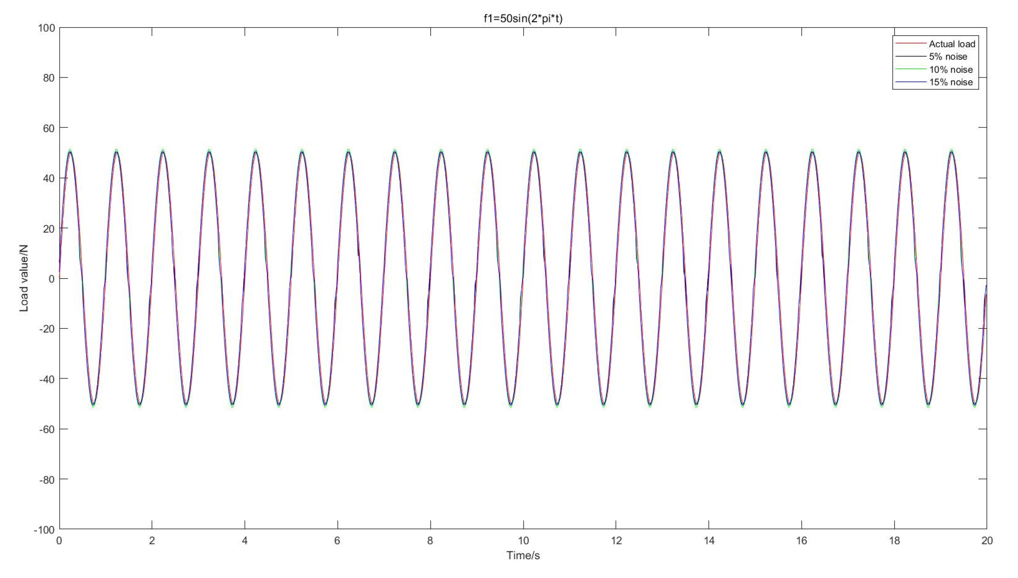
4. Experimental Verification

The correctness of the above theory is tested by experiments. In this experiment, a cantilever beam with a mass $m=0.5 \mathrm{kg}$ at the end, as shown in Figure 12, is used to simulate a single-degree-of-freedom system.

The specific parameters of the simulated SDOF system are shown in

Table 2. The parameters of the cantilever beam.

$\mathbf{Length}/\mathbf{m}$	$\mathbf{Width}/\mathbf{m}$	$\mathbf{Thickness}/\mathbf{m}$	$\mathbf{Elastic} \mathbf{Modulus}/\mathbf{GPa}$
0.5	0.02	0.002	200

, below.

According to the knowledge of mechanics of materials, the equivalent stiffness of cantilever beam to mass block in the loading direction is

$$k=\frac{3EI}{L^3}$$

(22)

where I is the moment of inertia of the beam section.

Based on Equation (22), the equivalent stiffness of spring $k=64 \mathrm{N}/\mathrm{m}$. The displacement and velocity signals of the mass block are collected by laser sensors, and the force signals are collected by force sensor and loaded by a vibration exciter. The sampling frequency of this experiment is 1024, and the time length of each micro segment is 0.01 s. The sampling duration is 20 s, and the applied excitation is $f=10\sin \left(10\pi t\right)$.

Table 3. The equipment details for the experiment.

Equipment Type	Model
Exciter	Labworks LW161.138
Displacement laser sensors	OptoNCDT 2310
Velocity laser sensors	Polytec PDV-100
Force sensors	PCB 208C03

shows the equipment details for the identification experiment.

The identification results are as follows.

It can be seen from the identification results in Figure 13 that there are still some errors between the identification results and the actual load. Through the error analysis of the identification results, it is found that the maximum error occurs at t = 4.6 s, and the error reaches 33%. The position with larger error is mainly concentrated in the extreme value of the actual load. The main reason for the errors is the experimental conditions—not only the noise in the environment but also the boundary condition of the cantilever beam cannot be idealized in the experiment. However, through global error statistics, it can be found that the mean-square error is about 5.78%. From this perspective, it can be considered that the experiment has verified the accuracy and the feasibility of the proposed dynamic-load identification method.

5. Conclusions

This paper proposed a novel method based on the function principle to solve the problem of load identification. According to the law of conservation of mechanical energy, the work done by the external load of the system is equal to the energy change of the system, so we established the equation between the unknown external load and the response of the discrete system. This method discretizes the overall time into several micro segments, and each micro segment can be regarded as a new beginning, so it can avoid the divergence of the identification result caused by the accumulated error in the time domain. From the above series of examples, it can be seen that this method can be used to identify a variety of different external load types, and the maximum value of errors is less than 5%, which meets the needs of engineering practice and has a certain degree of noise resistance. In addition, it can be seen from the above simulation that the accuracy of load identification has a certain relationship with the time interval of micro segments. The smaller the time interval, the higher the identification accuracy.

It should be pointed that this novel identification method requires every free displacement and velocity in the application process, which is more complicated in the implementation process, especially when there are many degrees of freedom. For continuous systems, it is difficult to obtain the change of kinetic energy and potential energy, so next we will try to solve the continuous system load-identification problem using the proposed method.

References

1. Yang, Z.; You, J. Identification Method of Dynamic Loads. J. Adv. Mech. 2015, 45, 29–54. [Google Scholar]
2. Qin, Y. Research on Application Technology of Dynamic Load Identification. Ph.D. Thesis, Nanjing University of Aeronautics and Astronautics, Nanjing, China, 2007. [Google Scholar]
3. Yang, Z.; You, Y. Research Progress of Dynamics Load Identification Method. Chin. J. Theor. Appl. Mech. 2015, 47, 384. [Google Scholar]
4. Hu, Y. Research on Load Identification Method Based on Least Square in Frequency Domain and Its Application. Ph.D. Thesis, Harbin Engineering University, Harbin, China, 2011. [Google Scholar]
5. Hu, J.; Zhang, X. An Optimization Method of Load Identification in Frequency Domain. J. Noise Vib. Control 2009, 29, 34–36. [Google Scholar]
6. Qin, Y. A Frequency Method: Two-dimension Distributed Load Identification. In Chinese Society of Theoretical and Applied Mechanics, Chinese Society of Vibration Engineering, Chinese Society of Aeronautics and Astronautics, Chinese Mechanical Engineering Society, Chinese Society of Astronautics. Abstract of Papers of the 9th National Conference on Vibration Theory and Application, Hangzhou, China, 17–19 October 2007; Chinese Society For Vibration Engineering: Nanjing, China, 2007; p. 2. [Google Scholar]
7. Zhou, P.; Zhang, Q.; Shuai, Z.; Li, W. Review of Research and Development Status of Dynamic Load Identification in Time Domain. J. Noise Vib. Control 2014, 34, 6–11. [Google Scholar]
8. Ma, X. Research of Some Issues of Dynamic Load Location Identification in Time Domain. Ph.D. Thesis, Nanjing University of Aeronautics and Astronautics, Nanjing, China, 2012. [Google Scholar]
9. Mao, Y. The Theoretical Approach and Experimental Study on the Inverse Problem of Dynamic Force Identification in Time Domain. Ph.D. Thesis, Dalian University of Technology, Dalian, China, 2010. [Google Scholar]
10. Jiang, J.; Luo, S.; Zhang, F. One novel dynamical calibration method to identify two-dimensional distributed load. J. Sound Vib. 2021, 515, 116465. [Google Scholar] [CrossRef]
11. Ory, H.; Glaser, H.; Holzdeppe, D. The Reconstruction of Forcing Function Based on Measured Structural Responses. In Proceedings of the 2nd International Symposium on Aeroelasticity and Structural Dynamics, Aachen, Germany, 1–3 April 1985. [Google Scholar]
12. Kreitinger, T.; Luo, H.L. Force Identification from Structural Response. In Proceedings of the 1987 SEM Spring Conference, Houston, TX, USA, 14–19 June 1987; pp. 851–855. [Google Scholar]
13. Lu, D.; Wu, M. Study on SWAT Method for Dynamic Load Identification. J. Vib. Impact 1999, 18, 78–82. [Google Scholar]
14. Chen, L.; Zhou, H. Weighted Acceleration Method of Dynamic Load Identification. J. Noise Vib. Control 2002, 14–16. [Google Scholar]
15. Doyle, J.F. A Wavelet Deconvolution Method for Impact Force Identification. J. Exp. Mech. Exp. Mech. 1997, 37, 403–408. [Google Scholar] [CrossRef]
16. Cheng, L.; Song, Z.; Wang, Z.; Ma, H. Impact Force Identification Based on Wavelet Deconvolution. J. Jinan Univ. (Nat. Sci. Ed.) 2008, 29, 443–446. [Google Scholar]
17. Gunawan, F.E.; Homma, H.; Kanto, Y. Two-step B-splines Regularization Method for Solving an Ill-posed Problem of Impact Force Reconstruction. J. Sound Vib. 2006, 297, 200–214. [Google Scholar] [CrossRef]
18. Hu, N.; Fukunaga, H.; Matsumoto, S.; Yan, B.; Peng, X.H. An Efficient Approach for Identifying Impact Force Using Embedded Piezoelectric Sensors. Int. J. Impact Eng. 2007, 34, 1258–1271. [Google Scholar] [CrossRef]
19. Gunawan, F.E.; Homma, H.; Morisawa, Y. Impact Force Estimation by Quadratic Spline Approximation. J. Solid Mech. Mater. Eng. 2008, 2, 1092–1103. [Google Scholar] [CrossRef]
20. Mao, Y.; Guo, X. Experiment Study on Dynamic Force Identification by a Parameter Estimation Method. In Proceedings of the SEM Annual Conference, Albuquerque, NM, USA, 1–4 June 2009; pp. 1–4. [Google Scholar]
21. Guo, X.; Mao, Y.; Zhao, Y. Research on Load Identification Based on Markov Parameter Precise Integration Method. J. Vib. Impact 2009, 28, 27–30. [Google Scholar]
22. Jiang, J.; Seaid, M.; Mohamed, M.S. Inverse algorithm for real-time road roughness estimation for autonomous vehicles. Arch. Appl. Mech. 2020, 90, 1333–1348. [Google Scholar] [CrossRef]
23. Hand, L.; Finch, J. Analytical Mechanics; Cambridge University Press: Cambridge, UK, 1998. [Google Scholar]
24. Jiang, J.; Ding, M.; Li, J. A novel time-domain dynamic load identification numerical algorithm for continuous systems. Mech. Syst. Signal Process. 2021, 160, 107881. [Google Scholar] [CrossRef]
Figure 1. Single-degree-of-freedom system.
Applsci 12 09623 g001
Figure 2. Single-degree-of-freedom system load identification.
Applsci 12 09623 g002
Figure 3. Multi-load of multiple-degree-of-freedom system.
Applsci 12 09623 g003
Figure 4. Multi-load identification of multi-DOF system.
Applsci 12 09623 g004
Figure 5. Single-degree-of-freedom system load-identification results.
Applsci 12 09623 g005
Figure 6. Load identification error comparison with Newmark method.
Applsci 12 09623 g006
Figure 7. Multiple-degree-of-freedom system load-identification results.
Applsci 12 09623 g007
Figure 8. f1 load-identification results.
Applsci 12 09623 g008
Figure 9. f2 load-identification results.
Applsci 12 09623 g009
Figure 10. f1 load identification with different noise levels.
Applsci 12 09623 g010
Figure 11. f2 load identification with different noise levels.
Applsci 12 09623 g011
Figure 12. Test-state diagram.
Applsci 12 09623 g012
Figure 13. Identification results.
Applsci 12 09623 g013