Abstract
Resilience has become an interesting parameter to assess the seismic risk connected with functionality of structures. In this regard, losses due to earthquakes may be significantly reduced by applying isolation at the base of the structures. However, design of isolation needs to consider the effects of soil deformability and all the connected effects of Soil Structure Interaction (SSI). In particular, soil deformability may reduce significantly the benefit of base isolation and thus the computation of resilience needs to consider such conditions. This paper aims to consider the issue by considering several isolated configurations on different soil conditions and for each of them, the seismic resilience has been computed. Numerical simulations have been performed in order to calculate the resilience of the various configurations and then this parameter was chosen a reference for comparing the isolation models on different soil conditions.
1. Background
Structural vulnerability to earthquakes may be significantly reduced by the application of base isolation, as demonstrated since the first studies by Kelly [1,2]. However, when isolation technique is applied on structures founded on deformable soil, its benefits may be reduced, as shown in [3,4,5,6,7]. Moreover, the role of Soil Structure Interaction (SSI) on base isolation has been assessed by experimental studies [8]. In this regard, SSI effects has been demonstrated [9,10,11] to consist of two important mechanisms: lengthening the structural periods and increasing the damping of the system. Moreover, [12] analyzed the interaction between SSI and base isolation (BI) by performing numerical analyses, ref. [13] studied the multi-story buildings with and without sliders in the cases of ground shock due to tunnel explosions. Spyrakos et al. [14,15] investigated the effect of SSI on the response of base-isolated buildings by considering equivalent fixed-base systems. In addition, ref. [16] assessed the local site conditions of the soil and their effects in the isolated structures.
In addition, since the first contribution by [17], seismic resilience has been applied as a parameter to assess the seismic performance of buildings. Moreover, ref. [18] defined resilience as the capacity to reduce the consequences of events, and to recover quickly from a damaged to an operational state. More recently, the resilience-based earthquake design initiative (REDi) rating system proposed a methodology to design resilient structures based on several criteria [19]. Many applications have been developed from this framework for assessing the seismic resilience of single structural configurations [20,21,22]. In particular, ref. [23] proposed an integrated approach to assess the seismic resilience of acute-care facilities with fragility functions.
In this background, there are still few contributions that assess the resilience of base isolated configurations. In particular, ref. [24] proposed a methodology to assess the seismic resilience of conventional and base-isolated steel structures by considering the aspects of sustainability (economic, social and environmental).
However, the assessment of the role of SSI on base isolated buildings by considering a resilience-based approach is still a hole in literature and thus the principal goal of this paper is to propose a framework that may calculate resilience of based-isolated structures founded on deformable soil.
In this regard, numerical simulations are performed with Opensees, enabling to consider the mutual effects of structural properties and soil deformations. In particular, the soil is represented with non-linear hysteretic materials and advanced plasticity models as to assess the mutual effects of BI and soil non-linearity at the same time. The models have been implemented in Opensees that may reproduce soil hysteretic elasto-plastic shear response, foundation impedances, realistic boundary conditions and advanced interface between the soil and the structure. The main objective is to assess these two dynamic mechanisms by investigating the cases where BI becomes detrimental. In particular, isolated structures on rigid soil are compared with the same structural schemes on soil with decreasing deformability showing the effects on the periods and on the damping of the performed systems.
In this regard, historically, ref. [25] showed that period elongation depends mainly on the so-called structure to soil stiffness ratio (depending on the height and the shear velocity of the flexible layer). Later, ref. [26] extensively investigated the formulas in ASCE 7-05 for several buildings by considering over 800 fundamental periods. Moreover, ref. [27] proposed an empirical formula for assessing the fundamental period of reinforced concrete structures by performing 3D numerical simulations of SSI effects. Additionally, ref. [28] investigated the effects of SSI on several residential RC buildings with different capacity design principles founded on four different soil conditions and applying 20 acceleration records. Other studies, such as refs. [29,30] proposed analytical surveys on the effects of SSI in terms of fundamental period and damping ratio. In addition, ref. [31] considered both experimental and numerical results and ref. [32] investigated the effects of SSI with a 1/4-scale steel-frame structure by reproducing 34 scenarios under fixed-base and flexible-base conditions. Moreover, the interaction between SSI and BI has been relatively studied in the literature. In this regard, ref. [12] analyzed the interaction between SSI and BI by performing numerical analyses, ref. [6] studied the multi-story buildings with and without sliders in the cases of ground shock due to tunnel explosions. Spyrakos et al. [14,15] investigated the effect of SSI on the response of base-isolated buildings by considering equivalent fixed-base systems.
This paper aims to overcome the previous literature, by proposing several novelties. (1) The interaction between base isolation (BI) and SSI effects are considered with advanced 3D numerical simulations, to capture the highly non-linear mechanisms between the soil, the foundation, the isolators and the superstructure. (2) The paper proposes a novel framework that consider resilience as the reference parameter. (3) The comparisons of the behaviour of the different configurations may be helpful for code provisions.
2. Case Studies
In order to investigate the relationships between base isolation and SSI effects, this paper investigates several configurations (see Table 1).

Table 1.
Performed models.
Model B1 represents a benchmark building with no isolation;
Model B2 consists of a base isolated systems with linear elastomeric bearings;
Model B3 consists of a base isolated models with non-linear isolators.
The models have been founded on a rigid slab foundation standing on a soil one-layer (depth: 30 m) mesh. The soil mesh is the same for all the models, in order to allow comparisons and the soil deformability has been varied by increasing the shear velocity from 80 m/s to 870 m/s (more details in Section 2.2).
2.1. Structural Models
The structure (Figure 1 and Figure 2) represents a low-rise stiff two-story (floor height: 3.2 m, total height: 6.4 m) reinforced concrete building with a 4 × 3 columns scheme (4 along the x-direction and 8 m spaced and 3 along y-direction and 6 m spaced, cross Area: 0.16 m2), designed in accordance with Eurocode 2 and 8 [33,34]. The hypothesis at the base of the structural model is that because of the presence of the isolation, the building may be assumed to be capacity designed being able to respond in the elastic range [35]. Therefore, the structure has been modelled with Elastic Beam Column elements (characteristics in Table 2). The masses calculated with the seismic combination following [34] were concentrated at each floor and included the structural components (such as beams, columns, slabs, balconies, stairs). The floors were modelled as rigid by applying the RigidDiaphragm [36], and thus the hypothesis of shear type behaviour was assumed (plan and vertical regularity has been assumed).
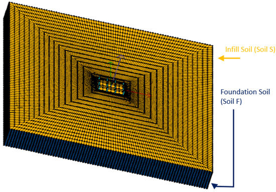
Figure 1.
3D view of the numerical model (Model B1, B2 and B3). Soil S: Infill soil (Yellow); Soil F: Foundation soil (Blue).
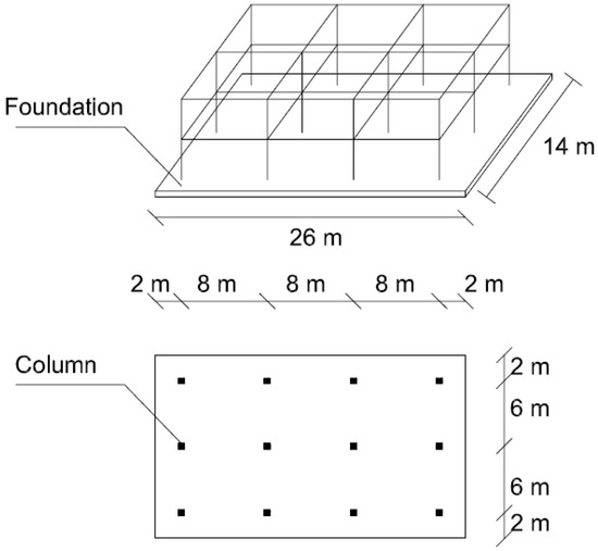
Figure 2.
Schematic view of the structure and the foundation (Model B1, B2 and B3).
Table 2.
Structural properties.
A superficial foundation (26 m × 14 m × 0.5 m, 15,264 nodes and 11,076 elements, Figure 2) has been simulated with a rigid concrete slab that may be considered typical for low-rise buildings with limited bearing pressures (180 kPa) at the base level, (see [37]). The slab was modeled with the Pressure Independent Multiyield (PIMY, [36,38], properties in Table 3) and was designed by considering the maximum eccentricity (the ratio between the overturning bending moment and the vertical axial forces) calculated with the minimum vertical loads (gravity and seismic loads) and maximum bending moments (due to the seismic loads). The PIMY is based on the Von Mises multi-surface kinematic plasticity model with an associate non-linear deviatoric part of the flow rule that is independent from the volumetric part (non-associate and linear-elastic). The backbone curves are defined by hyperbolic relations and described by two parameters (the strain shear modulus and ultimate shear strength). The interface between the structure and the foundation was modeled in order to represent the rocking component (rotations and over turning moments) that is fundamental to reproduce the SSI effects. The nodes of the last 50 cm of the columns were connected with horizontal rigid beam-column links (see [36]) to model the continuity of the link slab-column. EqualDOF constraint (see [36]) were used to connect the points (one belonging to the rigid link and the second to the foundation) in order to have the same displacements between the structure and the slab nodes. Zerolength elements (see [36]) were used to model the interface between the surrounding soil (named S soil) and the foundation by reproducing the uplifts and gapping mechanisms and non-linear effects (i.e., tilts and settlements) due to SSI. This assumption guaranteed to maintain the dynamic equilibrium at each step and thus resolving the convergence problems. The soil around the foundation (soil S) represents the infill weak soil and has been modeled with the Pressure Independent Multiyield (PIMY, [36,38]). The considered properties are shown in Table 3.
Table 3.
Geotechnical properties.
2.2. Soil Models
Soil F consists of a 30-m homogeneous layer modeled with the Pressure IndependMultiYield (PIMY) [38]. Table 3 shows the representative parameters, with increasing the shear velocity: 800 m/s (soil F1); 600 m/s (soil F2); 300 m/s (soil F3) and 100 m/s (soil F4), to consider the effects of soil deformability (total: 80 cases). The PIMY may consider the non-linear mechanisms of hysteretic response, radiation damping, amplitude-dependent amplifications and the accumulation of ground deformations (i.e., settlements, tilts and rotations). The soil domain (300 m × 300 m × 30 m) was modelled with a 3D soil mesh built up with 188,576 nodes and 177,940 non-linear ‘‘Bbar brick’’ elements that are configured with 20 nodes. These nodes represent the translational degrees of freedom (DOF, displacements along the three directions) and are recorded with Node Recorder (see [36,38]) at the corresponding integration points. The number of soil elements was defined by considering the minimum wavelength as the soil shear wave velocity (80 m/s) and the frequency of a typical seismic input motion (5 Hz) and thus the maximum element size was calculated by dividing the maximum wavelength by 24 (more details in [37]). The dimension of the elements was increased from the foundation to the end of the mesh. The lateral boundaries were considered to move in pure shear (see [39]) in order to represent free-field conditions. This assumption was verified by comparing the results with those of a free field case. The lateral boundaries were located far away from the foundation with the aim to reproduce an infinite soil domain. The boundary conditions were modeled by fixing the vertical directions for both the lateral boundaries (penalty method, with tolerance: 10−4, [37]) and the base that was set as a transmitting surface to remove the energy provided by the earthquakes from the mesh.
2.3. Isolation Models
The isolation system is located between the base of the column and the surface of the foundation (at z = 0.00 m) and it consists of 2 isolators for every column. The isolators (behaving in the longitudinal direction only) have been modelled very stiff in the other directions (vertical and transversal). They were designed following the methodology described in Section 10 of [34]:
- (1)
- Determination of the equivalent elastic stiffness of the device by assuming a target value for the period of the base isolated structure greater than the fundamental period of the fixed-base structure:where is the mass of the system and is the fundamental period of the isolated system.
- (2)
- The vertical loads under static and seismic conditions are calculated to choose the horizontal stiffness as well as its geometrical characteristics (diameter of the elastomer, total height of the isolator and the thickness of the elastomer); and the mechanical properties, such as the viscous damping of the rubber, the elasticity modulus, the maximum vertical load at the Ultimate Limit State, and the vertical load under seismic conditions.
- (3)
- The maximum displacements resulted from the analyses are finally compared with the design displacement, in order to verify the performance of the isolation.
The number of designed devices (2 at the base of each column) is determined to minimize the eccentricity between the center of the stiffness of the isolation system and the center of the mass of the superstructure. Two types of models were implemented for the isolators:
Model B2: implements a linear model (represented by equivalent linear springs), and Model B3: applies the simplified two-spring model (described in [2,40]) implemented inside Opensees by [41] and already applied in [42]. This model was assumed to consider the non-linear effects and the stability under large deformations.
Both the models were used in the longitudinal direction only, while in the other directions (transversal and vertical) high stiffness have been considered (3.5 × 10⁷ N/m2). It is worth noting that the properties of the two models (bearing stiffness) have been set up in order to have 2.5 s as the isolation period of the isolated system. The damping has been considered as 10% for both the models (see Table 3).
3. Resilience Calculation
Assessing the resilience of buildings is fundamental for the community itself, since if residential buildings are damaged in a non-operational way, people cannot stay in their houses and they need to find temporary housing in the same area or move or other areas, creating troubles within or between the communities. The same problem occurs when a business structure of a factory is damaged, there is a need to move shift staff and operations to other locations. In particular, realizing the balance between resilient structures and the necessary services is a duty for civil engineers in order to maintain post-earthquake functionality of communities.
In this paper the traditional formulation by [17] was used to calculate the seismic resilience of the structural configurations:
where:
t0E is the time of occurrence of the earthquake E,
RT is the repair time (RT) that is necessary to recover the original functionality;
Q(t) is the recovery function that describes the recovery process necessary to return to the pre-earthquake level of functionality (see Figure 3).
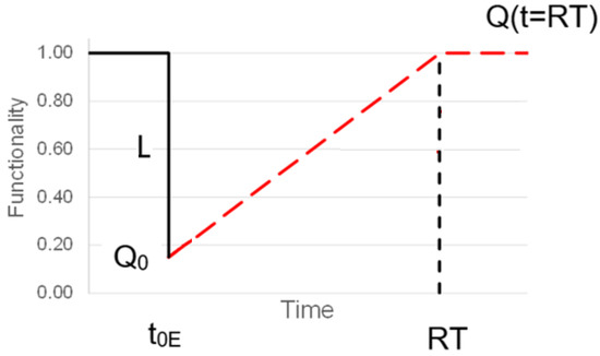
Figure 3.
Resilience calculation (L = losses; RT = repair time; Q = functionality).
Figure 3 shows that the formulation depends on several parameters:
- (1)
- L = losses (calculated as: L = 1 − Q0, where Q0 is the initial functionality)
- (2)
- RT: repair time to return to the original functionality.
These quantities are calculated with the Loss model and the Recovery model, proposed in the next subsections.
3.1. Loss Model
The paper proposes to calculate the losses on the definition of various limit states. In particular, four limit states (slight, moderate, extensive, complete) were selected by the technical literature [43] and by the previous contribution [37]. These limit states are based on the calculation of the longitudinal drifts of the structures. In particular, Slight, Moderate, Extensive and Complete damage states correspond with 0.30%, 0.60%, 1.50% and 4.00% (named LS1, LS2, LS3 and LS4), respectively. In correspondence with the exceedance of one LS, a specific value of L was assigned, as shown in Table 4. For example, if the calculated exceeds LS2, the assigned loss is 0.50, meaning that the functionality of the structure is reduced to a half of its original value.
Table 4.
Loss model.
3.2. Recovery Model
The recovery model is necessary in the calculation of resilience [17,44,45], but may be quite challenging to be realistically defined since it requires sufficient information from previous earthquakes. Analytical formulations are generally assumed and calibrated on the database of previous earthquakes. In this paper, two hypotheses were considered:
- (1)
- mobilization time [46] (that includes building inspection, site preparation, providing engineering services…) was neglected and thus the recovery function starts at the time of occurrence (t0E).
- (2)
- a linear recovery function was considered, as suggested by [17], when no sufficient information is available.
These two hypotheses may be considered the principal limitations of the model and may be object of future work.
Then, the calculation of repair time has been proposed in literature by several contributions. In particular, ref. [47] proposed a RT model consisting of two components: (1) Repair Scheduling and (2) Resource Scheduling. In addition, ref. [48] proposed a procedure to calculate RT, by considering the worker allocation and repair sequencing procedure. Both these approaches were introduced in order to overcome the well-established FEMA P-58 methodology [49]. Herein RT was calculated by following the simplified assumption that repair time is proportional with the drift ratio (the ratio between the maximum drift due to the seismic loads () and the design drift under static load conditions ()).
It is worth noting that the coefficient needs to be calibrated in order to represent the conditions that range between the case that the building is not repairable or uneconomical to repair the building (RT equal to replacing time) and the case of minor damage that does not compromise the structural operability (RT = 0).
3.3. Seismic Scenario
The seismic scenario consists of ten input motions selected from the NGA database in order to verify that the mean of the spectrum values of the sets of accelerograms is located between the −10% and +30% of the code-based spectrum, following the Eurocode 8 (2004) prescriptions, by considering the life-safety limit state (return period of 475 years, lat.: 42.333 N, 14.246 E, S = 1.50714, Tb = 0.257 s, Tc = 0.770 s, Td = 2.538, Cc = 2.02847), as shown in Figure 4. Table 5 shows the characteristics of the selected input motions in terms of peak ground acceleration (PGA).
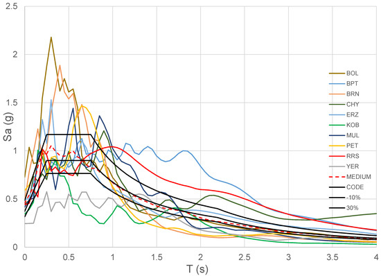
Figure 4.
Selected Input motions.
Table 5.
Selected input motion characteristics.
4. Results and Discussion
The results of the performed models for the four soil conditions are shown in Figure 5, Figure 6, Figure 7 and Figure 8 in terms of maximum longitudinal drifts for the considered seismic scenario. The limit states (LS1, LS2, LS3, LS4) are shown with horizontal lines in order to define the occurrence of exceedance. This condition is fundamental to derive the L on the basis of Table 4. In particular, Table 6 shows the state limits exceeded (for every configuration) deduced from the results (Figure 5, Figure 6, Figure 7 and Figure 8). In particular, the columns represent the condition of exceeding the four limit states for the selected models (models B1, B2 and B3 and for the foure soil conditions: F1, F2, F3 and F4).
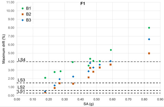
Figure 5.
Results: model B1, B2, B3 considering soil F1.
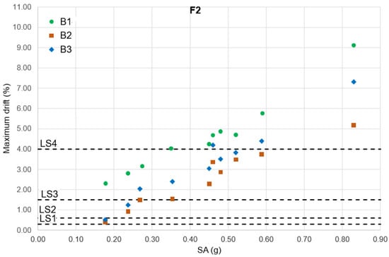
Figure 6.
Results: model B1, B2, B3 considering soil F2.
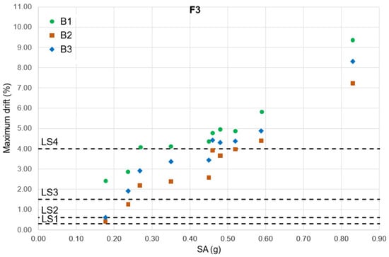
Figure 7.
Results: model B1, B2, B3 considering soil F3.
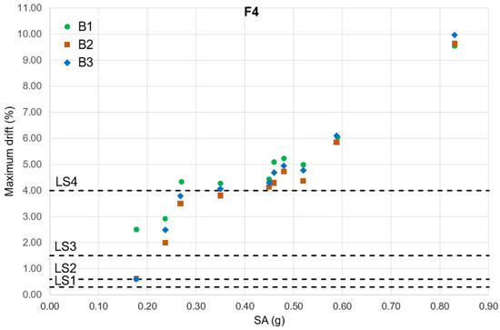
Figure 8.
Results: model B1, B2, B3 considering soil F4.
Table 7 shows the calculation of the losses, while Table 8 shows the RT resulted from the application of (2) by using a γ equal to 1. It is possible to see how RT increases with the intensities and how it varies for the 3 models. It is worth noticing that soil deformability plays an important role for increasing RT in case of model 1 (fixed case), white its effects are not linear for the other two models. It is also significant to consider that RT values for model 2 (linear model) are bigger than those obtained for model 3, since the role of non-linearity reduce the damage. Therefore, neglecting the non-linear mechanisms that occur in the bearings, is conservative, if compared with model 3, as previously demonstrated in [13,50].
Table 7.
Losses (L).
Table 8.
Repair Time (RT).
Table 9 shows the results in terms of Seismic Resilience (SR), and same observations regarding the dependency on the seismic intensity, the role of soil deformability and non-linear mechanisms of bearings in the quantification of SR. Figure 9 plots the last line of Table 9 in order to show the dependency of the SR with the soil deformability (in terms of Vs) for the most intense input motion (RRS) and by comparing the three models. It is worth noting that (1) isolation technique has beneficial effects in increasing the Seismic Resilience of the system (even if RT are bigger) and (2) the value of resilience does not significantly vary for model 1, while the trends for the isolated models differ significantly between each other. In particular, the best performance in terms of resilience seems to occur for model 2 (linear isolation) for deformable soils. However, this outcome is affected by the fact that non-linear mechanisms of the bearings are considered. Therefore, the more realistic model 3 shows that the isolation technique performs well at higher values of Vs (rigid soil). Smaller values of resilience at low intensities for model 3 are due to the interaction between the soil deformability and the isolator, that may become unconservative, as previously demonstrated in [13,50].
Table 9.
Seismic Resilience (SR): the last line (RRS) has been reproduced in Figure 9.
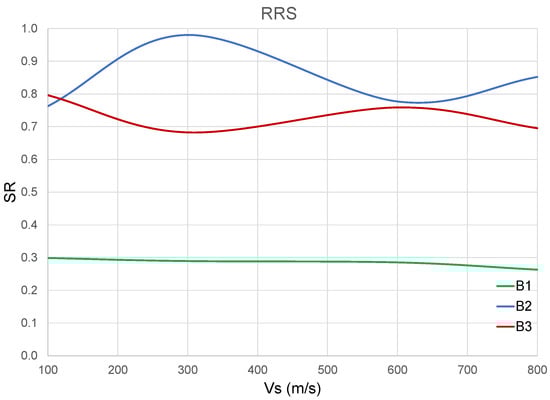
Figure 9.
Results in terms of Seismic Resilience for model B1, B2, B3 at various shear velocity for RRS motion (see last line of Table 9).
5. Conclusions
The paper proposes the quantification of Seismic Resilience for structural configurations by studying a case study that compares a fixed-base building and two isolated configurations. The main assumption is to assume resilience as the reference parameter to compare and discuss the performance of the various configurations. The results show the importance of considering soil deformability and non-linearity of the bearing in order to achieve realistic results. These outcomes may help taking decisions for design and/or recovery solutions for the buildings that are affected by the selected seismic scenarios. However, the results are limited to the analyzed 12 configurations (3 buildings and 4 foundation soils) and more studies are needed in order to generalize the outcomes. In this regard, Seismic Resilience was shown to be a comprehensive parameter that may represent the mechanisms of interaction between the soil, the structure and the bearings that are significant for design assessments. This paper is bases on the results of 12 configurations under 10 input motions (120 3D non-linear dynamic analyses). However, more case studies with different numerical models will be object of future analyses for a complete evaluation of the significance of the Seismic Resilience. In addition, the performance of the systems along the transversal and vertical direction will be investigated in future work.
Funding
This research received no external funding.
Institutional Review Board Statement
Not applicable.
Informed Consent Statement
Not applicable.
Data Availability Statement
Not applicable.
Conflicts of Interest
The author declares no conflict of interest.
References
- Kelly, J.M. Earthquake-Resistant Design with Rubber; Springer: London, UK, 1993. [Google Scholar]
- Naeim, F.; Kelly, J.M. Design of Seismic Isolated Structure—From Theory to Practice; Jonh Wiley & Sons Inc.: New York, NY, USA, 1999. [Google Scholar]
- Vlassis, A.; Spyrakos, C. Seismically Isolated Bridge Piers on Shallow Soil Stratum with Soil-Structure Interaction. Comput. Struct. 2001, 79, 2847–2861. [Google Scholar] [CrossRef]
- Tongaonkar, N.; Jangid, R. Seismic response of isolated bridges with soil-structure interaction. Soil Dyn. Earthq. Eng. 2003, 23, 287–302. [Google Scholar] [CrossRef]
- Ucak, A.; Tsopelas, P.A.M. Effect of soil-structure interaction on seismic isolated bridges. J. Struct. Eng. 2008, 134, 1154. [Google Scholar] [CrossRef]
- Tian, L.; Li, Z.-X. Dynamic response analysis of a building structure subjected to ground shock from a tunnel explosion. Int. J. Impact Eng. 2008, 35, 1164–1178. [Google Scholar] [CrossRef]
- Mina, D.; Forcellini, D. Soil–Structure Interaction Assessment of the 23 November 1980 Irpinia-Basilicata Earthquake. Geosciences 2020, 10, 152. [Google Scholar] [CrossRef]
- Haiyang, Z.; Xu, Y.; Chao, Z.; Dandan, Y. Shaking table tests for the seismic response of a base-isolated structure with the SSI effect. Soil Dyn. Earthq. Eng. 2014, 67, 208–218. [Google Scholar] [CrossRef]
- Kramer, S.L. Geotechnical Earthquake Engineering; Prentice Hall: Upper Saddle River, NJ, USA, 1996; p. 07458. [Google Scholar]
- Bhattacharya, K.; Dutta, S.C. Assessing lateral period of building frames incorporating soil-flexibility. J. Sound Vib. 2004, 269, 795–821. [Google Scholar] [CrossRef]
- Khalil, L.; Sadek, M.; Shahrour, I. Influence of the soil–structure interaction on the fundamental period of buildings. Earthq. Eng. Struct. Dyn. 2007, 36, 2445–2453. [Google Scholar] [CrossRef]
- Tsai, C.S.; Chen, C.-S.; Chen, B.-J. Effects of unbounded media on seismic responses of FPS-isolated structures. Struct. Control Health Monit. 2004, 11, 1–20. [Google Scholar] [CrossRef]
- Forcellini, D. The assessment of the interaction between Base Isolation (BI) technique and Soil Structure Interaction (SSI) effects with 3D numerical simulations. Structures, 2022; accepted. [Google Scholar]
- Spyrakos, C.; Koutromanos, I.; Maniatakis, C. Seismic response of base-isolated buildings including soil–structure interaction. Soil Dyn. Earthq. Eng. 2009, 29, 658–668. [Google Scholar] [CrossRef]
- Spyrakos, C.; Maniatakis, C.; Koutromanos, I. Soil–structure interaction effects on base-isolated buildings founded on soil stratum. Eng. Struct. 2009, 31, 729–737. [Google Scholar] [CrossRef]
- Fontara, L.K.; Titirla, M.; Wuttke, F.; Athanatopoulou, A.; Manolis, G.; Sextos, A. Multiple Support Excitation of a Bridge Based on a BEM Analysis of the Subsoil-Structure Interaction Phenomenon. In Proceedings of the 5th International Conference on Computational Methods in Structural Dynamics and Earthquake Engineering (COMPDYN), Creta Island, Greece, 25–27 May 2015. [Google Scholar]
- Cimellaro, G.P.; Reinhorn, A.M.; Bruneau, M. Seismic resilience of a hospital system. Struct. Infrastruct. Eng. 2010, 6, 127–144. [Google Scholar] [CrossRef]
- Bruneau, M.; Chang, S.E.; Eguchi, R.T.; Lee, G.C.; O’Rourke, T.D.; Reinhorn, A.M.; Shinozuka, M.; Tierney, K.; Wallace, W.A.; Von Winterfeldt, D. A Framework to Quantitatively Assess and Enhance the Seismic Resilience of Communities. Earthq. Spectra 2003, 19, 733–752. [Google Scholar] [CrossRef]
- Almufti, I.; Willford, M. The REDiTM Rating System: Resilience-Based Earthquake Design Initiative for the Next Generation of Buildings; Arup Co.: San Francisco, CA, USA, 2013. [Google Scholar] [CrossRef]
- Molina Hutt, C.; Almufti, I.; Willford, M.; Deierlein, G. Seismic loss and downtime assessment of existing tall steel-framed buildings and strategies for increased resilience. J. Struct. Eng. 2016, 142, C4015005. [Google Scholar] [CrossRef]
- Tian, Y.; Lu, X.; Lu, X.; Li, M.; Guan, H. Quantifying the seismic resilience of two tall buildings designed using Chinese and US Codes. Earthq. Struct. 2016, 11, 925–942. [Google Scholar] [CrossRef]
- Lu, X.; Xie, L.; Yu, C.; Lu, X. Development and application of a simplified model for the design of a super-tall mega-braced frame-core tube building. Eng. Struct. 2016, 110, 116–126. [Google Scholar] [CrossRef]
- Bruneau, M.; Reinhorn, A. Exploring the concept of seismic resilience for acute care facilities. Earthq. Spectra 2007, 23, 41–62. [Google Scholar] [CrossRef]
- Dong, Y.; Frangopol, D.M. Performance-based seismic assessment of conventional and base-isolated steel buildings including environmental impact and resilience. Earthq. Eng. Struct. Dyn. 2016, 45, 739–756. [Google Scholar] [CrossRef]
- Bielak, J. Dynamic behaviour of structures with embedded foundations. Earthq. Eng. Struct. Dyn. 1974, 3, 259–274. [Google Scholar] [CrossRef]
- Kwon, O.-S.; Kim, E.S. Evaluation of building period formulas for seismic design. Earthq. Eng. Struct. Dyn. 2010, 39, 1569–1583. [Google Scholar] [CrossRef]
- Hatzigeorgiou, G.D.; Kanapitsas, G. Evaluation of fundamental period of low-rise and mid-rise reinforced concrete buildings. Earthq. Eng. Struct. Dyn. 2013, 42, 1599–1616. [Google Scholar] [CrossRef]
- Oz, I.; Senel, S.M.; Palanci, M.; Kalkan, A. Effect of Soil-Structure Interaction on the Seismic Response of Existing Low and Mid-Rise RC Buildings. Appl. Sci. 2020, 10, 8357. [Google Scholar] [CrossRef]
- Avilés, J.; Pérez-Rocha, L.E. Influence of Foundation Flexibility on Rμ and Cμ Factors. J. Struct. Eng. 2005, 131, 221–230. [Google Scholar] [CrossRef]
- Avilés, J.; Suárez, M. Effective periods and dampings of building-foundation systems including seismic wave effects. Eng. Struct. 2002, 24, 553–562. [Google Scholar] [CrossRef]
- Luco, J.E. Bounds for natural frequencies, Dunkerley’s formula and application to soil–structure interaction. Soil Dyn. Earthq. Eng. 2013, 47, 32–37. [Google Scholar] [CrossRef]
- Xiong, W.; Jiang, L.Z.; Li, Y.Z. Influence of soil–structure interaction (structure-to-soil relative stiffness and mass ratio) on the fundamental period of buildings: Experimental observation and analytical verification. Bull. Earthq. Eng. 2016, 14, 139–160. [Google Scholar] [CrossRef]
- BS EN 1992-1-1:2004; Eurocode 2: Design of Concrete Structures—Part 1-1: General Rules and Rules for Buildings. British Standard Institution: London, UK, 2004.
- EN 1998-1:2004; Eurocode 8: Design of Structures for Earthquake Resistance—Part 1: General Rules, Seismic Actions and Rules for Buildings. European Committee for Standardization: Brussels, Belgium, 2005.
- Forcellini, D. A Novel Framework to Assess Soil Structure Interaction (SSI) Effects with Equivalent Fixed-Based Models. Appl. Sci. 2021, 11, 10472. [Google Scholar] [CrossRef]
- Mazzoni, S.; McKenna, F.; Scott, M.H.; Fenves, G.L. Open System for Earthquake Engineering Simulation, User Command-Language Manual; OpenSees Version 2.0; Pacific Earthquake Engineering Research Center, University of California: Berkeley, CA, USA, 2009; Available online: http://opensees.berkeley.edu/OpenSees/manuals/usermanual (accessed on 15 August 2022).
- Forcellini, D. Analytical fragility curves of shallow-founded structures subjected to sol structure interaction (SSI) effects. Soil Dyn. Earthq. Eng. 2021, 141, 106487. [Google Scholar] [CrossRef]
- Lu, J.; Elgamal, A.; Yang, Z. OpenSeesPL: 3D Lateral Pile-Ground Interaction, User Manual, Beta 1.0. 2011. Available online: http://soilquake.net/openseespl/ (accessed on 15 August 2022).
- Coleman, J.L.; Bolisetti, C.; Whittaker, A.S. Time-domain soil-structure interaction analysis of nuclear facilities. Nucl. Eng. Des. 2016, 298, 264–270. [Google Scholar] [CrossRef]
- Forcellini, D.; Kelly, J.M. The analysis of the large deformation stability of elastomeric bearings. J. Eng. Mech. ASCE 2014, 140, 04014036. [Google Scholar] [CrossRef]
- Ryan, K.L.; Kelly, J.M.; Chopra, A.K. Nonlinear model for lead-rubber bearings including axial-load effects. J. Eng. Mech. 2005, 131, 1270–1278. [Google Scholar] [CrossRef]
- Forcellini, D. Cost assessment of isolation technique applied to a benchmark bridge with soil structure interaction. Bull. Earthq. Eng. 2017, 15, 51–69. [Google Scholar] [CrossRef]
- Holmes, W. Multi-Hazard Loss Estimation Methodology, Technical Manual; Federal Emergency Management Agency (FEMA): Washington, DC, USA, 2003.
- Mieler, M.W.; Mitrani-Reiser, J. Review of the State of the Art in Assessing Earthquake-Induced Loss of Functionality in Buildings. J. Struct. Eng. 2018, 144, 04017218. [Google Scholar] [CrossRef]
- Sun, L.; Stojadinovic, B.; Sansavini, G. Resilience Evaluation Framework for Integrated Civil Infrastructure-Community Systems under Seismic Hazard. arXiv 2019, arXiv:1901.06465. [Google Scholar] [CrossRef]
- Comerio, M.C. Estimating downtime in loss modeling. Earthq. Spectra 2006, 22, 349–365. [Google Scholar] [CrossRef]
- Terzic, V.; Villanueva, P.K.; Saldana, D.; Yoo, D.Y. Framework for modelling post-earthquake functional recovery of buildings. Eng. Struct. 2021, 246, 113074. [Google Scholar] [CrossRef]
- Molina Hutt, C.; Vahanvaty, T.; Kourehpaz, P. An analytical framework to assess earthquake-induced downtime and model recovery of buildings. Earthq. Spectra 2022, 38, 1283–1320. [Google Scholar] [CrossRef]
- Federal Emergency Management Agency (FEMA). Seismic Performance Assessment of Buildings (FEMA P-58); FEMA: Washington, DC, USA, 2018.
- Forcellini, D. Seismic assessment of a benchmark based isolated ordinary building with soil structure interaction. Bull. Earthq. Eng. 2018, 16, 2021–2042. [Google Scholar] [CrossRef]


Publisher’s Note: MDPI stays neutral with regard to jurisdictional claims in published maps and institutional affiliations. |
© 2022 by the author. Licensee MDPI, Basel, Switzerland. This article is an open access article distributed under the terms and conditions of the Creative Commons Attribution (CC BY) license (https://creativecommons.org/licenses/by/4.0/).