Design of Optical Tweezers Manipulation Control System Based on Novel Self-Organizing Fuzzy Cerebellar Model Neural Network

Abstract

Holographic optical tweezers have unique non-physical contact and can manipulate and control single or multiple cells in a non-invasive way. In this paper, the dynamics model of the cells captured by the optical trap is analyzed, and a control system based on a novel self-organizing fuzzy cerebellar model neural network (NSOFCMNN) is proposed and applied to the cell manipulation control of holographic optical tweezers. This control system consists of a main controller using the NSOFCMNN with a new self-organization mechanism, a robust compensation controller, and a higher order sliding mode. It can accurately move the captured cells to the expected position through the optical trap generated by the holographic optical tweezers system. Both the layers and blocks of the proposed NSOFCMNN can be adjusted online according to the new self-organization mechanism. The compensation controller is used to eliminate the approximation errors. The higher order sliding surface can enhance the performance of controllers. The distances between cells are considered in order to further realize multi-cell cooperative control. In addition, the stability and convergence of the proposed NSOFCMNN are proved by the Lyapunov function, and the learning law is updated online by the gradient descent method. The simulation results show that the control system based on the proposed NSOFCMNN can effectively complete the cell manipulation task of optical tweezers and has better control performance than other neural network controllers.

1. Introduction

In modern biomedical engineering, the micro-manipulation of biological cells has become a hot research object. At present, atomic force microscopy (AFM) [1], microstraw technology [2], dielectrophoretic traps [3], magnetic tweezers [4] and other micromanipulation techniques have been applied to the manipulation of biological cells. Holographic optical tweezers, because of their unique non-physical contact and flexibility, do not have the disadvantage that micro-straw technology may damage the structure of cells, nor do magnetic tweezers lack the flexibility needed to control biological cells alone. It can sort [5], transport [6] and perform other complex micro-operations [7,8,9,10,11,12] for cells, and thus plays an increasingly important role in micro-manipulation. In recent years, many seniors have conducted in-depth research on single-cell manipulation [13,14,15]. However, the manipulation of single cells using holographic optical tweezers has always been challenging to meet the needs of more advanced practical applications. Multicellular manipulation can achieve more complex and more efficient practical tasks, such as using an optical trapping force to gather multiple red blood cells to block blood vessels, or using optical forceps to pull red blood cells to dredge blocked capillaries [6].

In the manipulation of optical tweezers, some scholars use PI control and PID control [16,17]; however, it is still possible to improve control performance further. With the research and development of neural networks, more and more neural networks have been applied to various projects as controllers in recent years [18,19,20]. On the other hand, the use of fuzzy theory can effectively reflect the inaccurate data in reality [21]. Many papers have carried out further research on fuzzy mathematics [22], fuzzy inference [23] and other related issues [24,25,26]. Regarding the fuzzy cerebellar model neural network (FCMNN), because fuzzy rules are added to the cerebellum model, the neural network has the advantages of local fast approximation of cerebellar neural network and strong generalization of fuzzy rules to data. In various engineering experiments, such as multi-dimensional classification, signal processing, approximation and other control issues [27,28,29,30,31,32], after many studies of verification by predecessors, it currently possesses a good approximation ability to uncertain linear systems. Therefore, this paper considers the application of FCMNN in cell manipulation to improve the accuracy of cell manipulation.

In most cases, it is not possible for FCMNN to obtain the appropriate structure directly. The size of the storage space is difficult to determine, which will affect the learning effect of the network. Therefore, some FCMNNs with self-organizing characteristics are proposed [33,34,35]. However, these FCMNNs have problems such as complex methods, a weak ability to adapt to online real-time, and no analysis of structure deletion. Aiming at mitigating these deficiencies, a NSOFCMNN is proposed in this paper, which can change the number of layers and blocks of the network with clearer self-organizing rules, and adjust it online in real time.

Due to the inefficiency of single-cell manipulation, cell manipulation experiments require high control accuracy, and it is difficult for the control performance of traditional controllers to meet the current experimental needs. The purpose of this paper is to study an efficient and precise control method for manipulating cells in a holographic optical tweezers system to improve the above problems. The dynamics model of the cells captured by the optical trap produced by holographic optical tweezers is analyzed. Combining the advantages of NSOFCMNN and the higher order sliding-mode control, a control system based on NSOFCMNN with a new self-organization mechanism is proposed. It includes a NSOFCMNN main controller, a robust compensator, and a higher order sliding surface. The number of layers and blocks of the NSOFCMNN can be adaptively increased or decreased according to the error between the real-time position of the cell and the expected position. The robust compensation controller is used to cope with the chattering and to eliminate the approximation error. The higher order sliding mode surface is used to effectively deal with the external disturbances and the chattering. The holographic optical tweezers system can obtain and operate the positions of multiple cells at the same time, and the position of each optical trap can be controlled independently [9]. Therefore, this control system can accurately manipulate the biological cell to move to the expected position through the optical trap generated by multiple holographic optical tweezers. After considering the expected interval between cells, the cooperative control of multiple cells by holographic optical tweezers is further realized. Taking the yeast cell as an example, through the MATLAB simulation experiment, it has been verified that the control system with the NSOFCMNN as the controller proposed in this paper can effectively complete the control of holographic optical tweezers for a single yeast cell and cooperative control for multiple yeast cells. It can meet the requirements of manipulating any number of cells in different experiments, and can improve the efficiency of cell manipulation. By comparing the root mean square error (RMSE) and mean absolute error (MAE) of other neural network controllers, the SOFCMNN proposed in this paper stands out, with smaller index values and better control performance.

The rest of this paper is organized as follows. Section 2 describes the fuzzy rules, the structure, the updating laws and the new self-organizing mechanism of the NSOFCMNN. In Section 3, the holographic optical tweezers system is introduced, the controlled cell dynamics model is analyzed, the cell manipulation control system based on the proposed NSOFCMNN is designed, and the convergence is proven by the Lyapunov function. In Section 4, the simulation experiments and the result analyses are carried out to verify the effectiveness of the proposed control system. Section 5 presents the conclusion and the future research direction.

2. Model of NSOFCMNN

2.1. Fuzzy Rules of the NSOFCMNN

NSOFCMNN is improved by adding fuzzy rules on the basis of the cerebellar model network. The fuzzy cerebellar model network in this paper has a layer structure and a block structure, and its fuzzy reasoning is realized by a type-1 fuzzy system. The fuzzy rules are listed in Equation (1) as follows:

$$\begin{gathered} {\Re }^h:\mathrm{If} p_1\mathrm{is} {\zeta }_{1jk} \mathrm{and} p_2 \mathrm{is} {\zeta }_{2jk},\dots , p_{n_i} \mathrm{is} {\zeta }_{n_{i}jk} \mathrm{then} O_o={\omega }_{jko}, \\ \mathrm{for} j=1,2,\dots ,n_j,k=1,2,\dots ,n_k,o=1,2,\dots ,n_o,h=1,2,\dots ,n_h \end{gathered}$$

(1)

where $n_i$ and $n_o$ represent the number of dimensions of input and output, $n_j$ is the number of network layers for each input, and $n_k$ is the number of blocks for each layer. $n_h=n_j{n}_k$ is the number of fuzzy rules. ${\zeta }_{ijk}$ is the fuzzy set of the $i$th input, $j$th layer and $k$th block. ${\omega }_{jko}$ is the $o$th output weight.

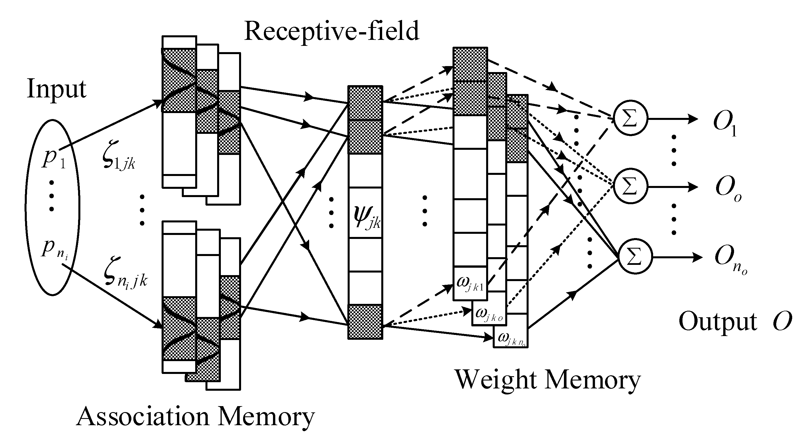
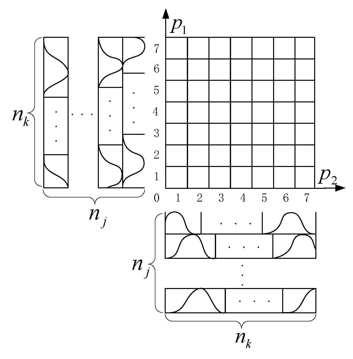
2.2. Structure of the NSOFCMNN

The structure of the proposed NSOFCMNN is shown in Figure 1.

NSOFCMNN has a five-layer structure.

The first layer is the input space, where $\mathit{P}$ is the input data, $\mathit{P}={\left[p_1,p_2,\dots ,p_{n_i}\right]}^T$.

The second layer is the numerical space after fuzzification of the input data, also known as “Association Memory” space which is a hyperspace. A fuzzy membership function, also known as the basis function, is added to each block of each layer, as shown in Equation (2). Each input data will be obfuscated and stored in blocks in different layers, as shown in Figure 2.

$$\begin{gathered} {\zeta }_{ijk}=\exp \left[\frac{-{\left(p_i-a_{ijk}\right)}^2}{{\beta }_{ijk}{}^2}\right], \\ for i=1,2,3,\cdots ,n_i \end{gathered}$$

(2)

where ${\alpha }_{ijk}$ is the central value of the $i$th input, $j$th layer and the $k$th block of the Gaussian function, and ${\beta }_{ijk}$ is the variance of the $i$th input, the $j$th layer and the $k$th block of a Gaussian function.

The third layer is the “Receptive-field” space, which consists of multiple receptive fields. Each receptive field also has a layer and a block. After the blocks activated by the same layer are accumulated, they correspond to a weight address space, so it is also called a weight value address space. Among them, each receptive field ${\psi }_{jk}$ is related to the $j$th layer and the $k$th block.

$$\begin{gathered} {\psi }_{jk}={\displaystyle \prod }_{i=1}^{n_i}{\zeta }_{ijk}={\displaystyle \prod }_{i=1}^{n_i}\exp \left[\frac{-{\left(p_i-a_{ijk}\right)}^2}{{\beta }_{ijk}{}^2}\right], \\ for i=1,2,3,\cdots ,n_i,j=1,2,3,\cdots ,n_j, \\ and k=1,2,3,\cdots ,n_k \end{gathered}$$

(3)

The fourth layer is the “Weight Memory” space, where ${\omega }_{jko}$ is a hypercube representing the weights required to compute the output of each dimension.

$$\begin{gathered} {\mathit{\omega }}_0=\left[{\omega }_{11o},\cdots ,{\omega }_{1n_{k}o},{\omega }_{21o},\cdots ,{\omega }_{1n_{k}o},\right. \\ {\left.\cdots ,{\omega }_{n_{j}1o},\cdots ,{\omega }_{n_j{n}_{k}o}\right]}^T\in {\Re }^{n_j{n}_k}, \\ for o=1,\cdots ,n_o \end{gathered}$$

(4)

The fifth layer is the output layer, and the output $O_o$ is obtained by solving the algebraic sum of the activated values of the “Receptive-field” space and “Weight Memory” space of each block in each layer. This is actually a defuzzification process.

$$\begin{gathered} u_{{\mathrm{NSOFCMNN}}_o}=O_o={\mathit{\omega }}_o^T\mathit{\psi }={\displaystyle \sum }_{j=1}^{n_j}{\displaystyle \sum }_{k=1}^{n_k}{\omega }_{jko}{\psi }_{jk}, \\ for j=1,2,3,\cdots ,n_j, k=1,2,3,\cdots ,n_k, \\ and o=1,\cdots ,n_o \end{gathered}$$

(5)

2.3. Updating Law

In terms of updating the weights of the neural network of the fuzzy cerebellum model, the ${\psi }_{jk}$ and ${\omega }_{jko}$ values need to be updated, and the gradient descent method is used here. First, the error function E(k) is defined, as shown in (6):

$$E\left(k\right)=\frac{1}{2}{\displaystyle \sum }_{o=1}^{n_o}{\left(O{d}_o\left(t\right)-O_o\left(t\right)\right)}^2=\frac{1}{2}{\displaystyle \sum }_{o=1}^{n_o}{\mathit{\epsilon }}_0{}^2\left(t\right)$$

(6)

where ${\epsilon }_0\left(t\right)=O{d}_o\left(t\right)-O_o\left(t\right)$ represents the difference between the expected output $O{d}_o$ and the actual output $O_o$ of the fuzzy cerebellar model neural network. After calculating ${\mathit{\epsilon }}_0$, the updated formula of ${\omega }_{jko}$ is derived as:

$$\begin{array}{ll}\mathsf{\Delta }{\omega }_{jko}& =-{\kappa }_{\omega }\frac{\mathit{\partial }E}{\mathit{\partial }{\omega }_{jko}}=-{\kappa }_{\omega }\frac{\mathit{\partial }E}{\mathit{\partial }{O}_o}\frac{\mathit{\partial }{O}_o}{\mathit{\partial }{\omega }_{jko}}\\ & ={\kappa }_{\omega }{\displaystyle {\displaystyle \sum }_{o=1}^{n_o}}{\epsilon }_o{\psi }_{jk}\end{array}$$

(7)

$${\omega }_{jko}(t+1)={\omega }_{jko}\left(t\right)+\mathsf{\Delta }{\omega }_{jko}\left(t\right)$$

(8)

where ${\kappa }_{\omega }$ is the learning rate of weight $\omega$. The new ${\omega }_{jko}$ will be derived through $\mathsf{\Delta }{\omega }_{jko}$. The center value ${\alpha }_{ijk}$ and the width value ${\beta }_{ijk}$ of the Gaussian basis function applied in the “Association Memory” space are updated by (9) and (10).

$$\begin{gathered} \mathsf{\Delta }{\alpha }_{ijk}=-{\kappa }_{\alpha }{\displaystyle \sum }_{o=1}^{n_o}\frac{\mathit{\partial }E\left(t\right)}{\mathit{\partial }{\alpha }_{ijk}}=-{\kappa }_{\alpha }{\displaystyle \sum }_{o=1}^{n_o}\frac{\mathit{\partial }E}{\mathit{\partial }{O}_o}\frac{\mathit{\partial }{O}_o}{\mathit{\partial }{\psi }_{jk}}\frac{\mathit{\partial }{\psi }_{jk}}{\mathit{\partial }{\alpha }_{ijk}} \\ ={\kappa }_m{\displaystyle \sum }_{o=1}^{n_o}{\epsilon }_o{\omega }_{jko}{\psi }_{jk}2\left(p_i-{\alpha }_{ijk}\right){\beta }_{ijk}{}^{-2} \end{gathered}$$

(9)

$$\begin{gathered} \mathsf{\Delta }{\beta }_{ijk}=-{\kappa }_{\beta }{\displaystyle \sum }_{o=1}^{n_o}\frac{\mathit{\partial }E\left(t\right)}{\mathit{\partial }{\beta }_{ijk}}=-{\kappa }_{\beta }{\displaystyle \sum }_{o=1}^{n_o}\frac{\mathit{\partial }E}{\mathit{\partial }{O}_o}\frac{\mathit{\partial }{O}_o}{\mathit{\partial }{\psi }_{jk}}\frac{\mathit{\partial }{\psi }_{jk}}{\mathit{\partial }{\beta }_{ijk}} \\ ={\kappa }_{\beta }{\displaystyle \sum }_{o=1}^{n_o}{\epsilon }_o{\omega }_{jko}{\psi }_{jk}2{\left(p_i-{\alpha }_{ijk}\right)}^2{\beta }_{ijk}{}^{-3} \end{gathered}$$

(10)

In Equations (9) and (10), ${\kappa }_{\alpha }$ and ${\kappa }_{\beta }$ represent the update learning rate of the Gaussian basis function center value α and variance value β, respectively, and the update formula is shown in Equations (11) and (12):

$${\alpha }_{jko}\left(t+1\right)={\alpha }_{jko}\left(t\right)+\mathsf{\Delta }{\alpha }_{jko}\left(t\right)$$

(11)

$${\beta }_{jko}\left(t+1\right)={\beta }_{jko}\left(t\right)+\mathsf{\Delta }{\beta }_{jko}\left(t\right)$$

(12)

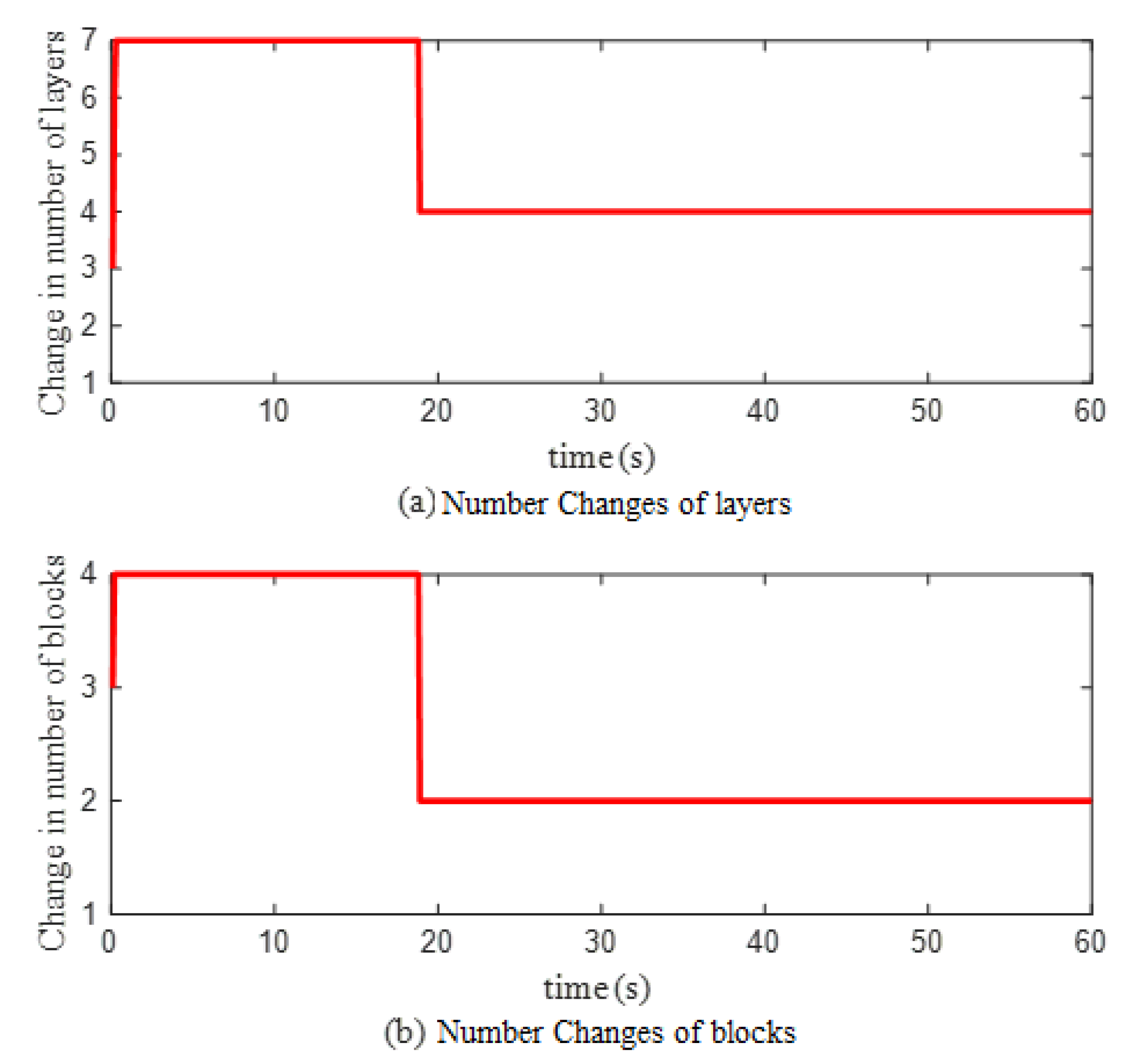
2.4. Novel Self-Organizing Adjustment Mechanism

This paper proposes a new self-organization adjustment mechanism that can automatically adjust the number of layers and blocks of the NSOFCMNN according to the size of the input data.

For a traditional FCMNN, most of them set a fixed number of network layers $n_j$ and blocks $n_k$ to improve the generalization ability and learning accuracy of the fuzzy cerebellar model neural network. However, for different input data $\mathit{P}$, the fixed number of layers and blocks cannot obtain a better learning effect. When a neural network has a large amount of input data with a wide range of values, a small number of layers or blocks cannot approximate the ideal output well, and the number of layers and blocks of the network needs to be increased. However, when a small amount of data with a small value range is obtained, the large number of layers or blocks will slow down the operation speed of the neural network of the cerebellar model, and the learning efficiency is not ideal. At this time, it is necessary to consider reducing redundant blocks or redundant layers.

Therefore, a novel self-organizing adjustment mechanism is established in this section. According to these rules, it is determined whether the number of layers and blocks need to be increased or decreased. If not, it means that the number of layers and blocks at this time are ideal values.

(1) Increase the number of layers and blocks

For constructing a self-organizing fuzzy cerebellum model neural network, it is first necessary to put in place a set of rules to judge and determine whether to add a new number of layers and blocks in the “Association Memory” space, and at the same time create a hypercube of new layers and blocks in the network part of the “Weight Memory” space and the part of the new layer and block corresponding to the “Weight Memory” space. The number of existing layers and blocks can be described as clusters. Depending on the input data, if the input data fall within the range of the cluster, it means that the input data belong to the current cluster, and there is no need to add new layers and blocks. There are layers and blocks and other rules to update.

In the “Associative Memory” layer, the average distance $\mathit{A}{\mathit{R}}_{jk}$ is defined as:

$$\begin{gathered} \mathit{A}{\mathit{R}}_{jk}\left(\mathit{P}\right)={\Vert \mathit{P}-{\mathit{\alpha }}_{jk}\Vert }_2 \\ for j=1,2,\cdots ,n_j, k=1,2,\cdots ,n_k \end{gathered}$$

(13)

where $\mathit{\alpha }={\left[{\alpha }_{1jk},\cdots ,{\alpha }_{ijk}\right]}^T,i=1,\cdots ,n_i.$ Using the MAX-MIN method, the average distance $\mathit{A}{\mathit{R}}_{jk}$ of each layer and each block is traversed to determine whether to increase the number of layers.

$$\mathit{g}=\arg \underset{1\le j\le n_j}{\min } \underset{1\le k\le n_k}{\min }\mathit{A}{\mathit{R}}_{jk}\left(\mathit{P}\right)$$

(14)

where $\mathit{g}=\left(\widehat{j},\widehat{k}\right)$, $\widehat{j}$ and $\widehat{k}$ represent the $\widehat{j}$th layer and the $\widehat{k}$th block to which the smallest block in these blocks belongs among all the blocks with the smallest average distance in each layer. By setting a minimum value $T_n$, if $\mathit{A}{\mathit{R}}_{\mathit{g}}\left(\mathit{P}\right)>T_n$ is satisfied, that is, in the blocks with the smallest average distance of each layer corresponding to all inputs, the average distance $\mathit{A}{\mathit{R}}_{jk}$ of the smallest blocks in these blocks, if in all input dimensions, is the largest $\mathit{A}{\mathit{R}}_{jk}$ If it is greater than or equal to $T_n$, a new layer node and block node are generated at the same time.

$$\underset{i}{\max }\mathit{A}{\mathit{R}}_{\widehat{j}\widehat{k}}\left(\mathit{P}\right)\ge T_n$$

(15)

This method means that if the distance between the input data and the center of the existing layer nodes in the cluster is greater than the set minimum value, the number of layers and blocks at the moment is too small, and a new one needs to be generated. The new number of layers and blocks are given by:

$$n_j\left(t+1\right)=n_j\left(t\right)+1$$

(16)

$$n_k\left(t+1\right)=n_k\left(t\right)+1$$

(17)

where $n_j\left(t\right)$ is the number of existing layers and $n_k\left(t\right)$ is the number of existing blocks. After new layers and blocks are generated, not only the layers and blocks of the “Associative Memory” space will be added, but also the layers and blocks of the receptive field will also increase. The center value and variance value of the Gaussian function will add new layer nodes and block nodes. The values of the new layer and block corresponding to the two parameters are set as:

$${\alpha }_{i{n}_j{n}_k}=p_i$$

(18)

$${\beta }_{ijk}={\beta }_{i{n}_{\widehat{j}}{n}_{\widehat{k}}}$$

(19)

(2) Reduce the number of layers

The main purpose of reducing the layers is to improve the operation speed of the NSOFCMNN, and also use the MAX-MIN method to delete the redundant layers. Consider the $j$th layer value of the $o$th output:

$$O_{oj}={\displaystyle \sum }_{k=1}^{n_k}{\omega }_{jko}{\psi }_{jk},o=1,\cdots ,n_o,j=1,2,\cdots ,n_j$$

(20)

In formula (5), $O_o$ is the output of the $o$th dimension. In formula (20), $O_{oj}$ is the multiplication and summation of the “Receptive-field” space and “Weight Memory” space of the $j$th layer of the $o$th dimension. Next, the contribution ratio value $\mathit{R}{\mathit{R}}_{oj}$ is defined as:

$$\begin{gathered} \mathit{R}{\mathit{R}}_{oj}\left(\mathit{P}\right)=\frac{O_{oj}\left(\mathit{P}\right)}{O_o\left(\mathit{P}\right)} \\ for o=1,\cdots ,n_o, j=1,2,\cdots ,n_j \end{gathered}$$

(21)

$\mathit{R}{\mathit{R}}_{oj}\left(\mathit{P}\right)$ represents the proportion of the output in the entire $o$ dimension after the input data is transformed into the “Receptive-field” space of the fuzzy cerebellar model neural network and multiplied by the weight of the “Weight Memory” space of the jth layer. Therefore, the largest contribution layer of all output dimensions is found, and the layer $\widehat{\varphi }$ with the smallest contribution is:

$$\widehat{\varphi }=\arg \underset{1\le j\le n_j}{\min } \underset{1\le o\le n_o}{\max }\mathit{R}{\mathit{R}}_{oj}\left(\mathit{P}\right)$$

(22)

By setting a minimum contribution value $T_m$ of the layer, if $\mathit{R}{\mathit{R}}_{o\widehat{\varphi }}\le T_m$ is satisfied, which means that for the $o$th dimension output, the contribution of a certain layer to the output is less than a set minimum contribution value, then the $\widehat{\varphi }$th layer at this moment is considered redundant and it should be deleted. At the same time, the corresponding layers of “Associative Memory” space, “Weight Memory” space and the center value and variance value of the Gaussian function will be reduced, and then the parameters will be updated according to the update formula. At this time, the new number of layers is given by:

$$n_j\left(t+1\right)=n_j\left(t\right)-1$$

(23)

(3) Reduce the number of blocks

The rules for reducing blocks have similar logic to the rules for reducing layers. Using the MAX-MIN method, the value h of the $o$th output at the $k$th block in the $j$th layer is considered as follows:

$$O_{ojk}={\omega }_{jko}{\psi }_{jk},o=1,\cdots ,n_o,j=1,2,\cdots ,n_j$$

(24)

The contribution ratio value $\mathit{K}{\mathit{K}}_{ojk}$ is defined as:

$$\begin{gathered} \mathit{K}{\mathit{K}}_{ojk}\left(\mathit{P}\right)=\frac{O_{ojk}\left(\mathit{P}\right)}{O_{oj}\left(\mathit{P}\right)} \\ for o=1,\cdots ,n_o, j=1,2,\cdots ,n_j \\ and k=1,2,\cdots ,n_k \end{gathered}$$

(25)

$\mathit{K}{\mathit{K}}_{ojk}\left(\mathit{P}\right)$ represents the ratio of the input data after passing through the “Receptive-field” space of NSOFCMNN and the corresponding weight of the “Weight Memory” space of the kth block multiplied in the $j$th layer of the entire oth dimension. Then, the block with the largest proportion in the output of the $j$th layer of the oth dimension is found. After that, the block $\widehat{c}$ with the smallest proportion among the blocks with the largest proportion of each layer in the $o$th dimension is found, and finally the block $\widehat{\phi }$ with the smallest proportion among all the blocks $\widehat{c}$ with the smallest proportion in the $n_o$ dimension is found, and $\widehat{\phi }$ is expressed as:

$$\widehat{\phi }=\arg \underset{1\le o\le n_o}{\min } \underset{1\le j\le n_j}{\min } \underset{1\le k\le n_k}{\max }\mathit{K}{\mathit{K}}_{ojk}\left(\mathit{P}\right)$$

(26)

A minimum contribution value $T_k$ of block is set, if $\mathit{K}{\mathit{K}}_{oj\widehat{\phi }}\le T_k$ is satisfied. This means that, for the blocks of all the layers in the output, the contribution value of the smallest block in the blocks with the largest proportion of each layer is less than $T_k$, then the $\widehat{\phi }$th block number is considered a redundant block and it should be deleted at this moment. The number of blocks in the corresponding “Associative Memory” space, the “Weight Memory” space, as well as the center value and the variance value of the Gaussian function will be reduced, and then the parameters will be updated according to the update formula. The new number of blocks at this time is given by:

$$n_k\left(t+1\right)=n_k\left(t\right)-1$$

(27)

3. Cell Manipulation Control

3.1. Holographic Optical Tweezers System

The holographic optical tweezers system controls the hologram generated by the computer loaded on the spatial light modulator (SLM) by programming, then controls the SLM to carry out phase modulation, divides a single beam of incident light into multiple outgoing beams, and finally produces a large array of light traps. The dynamic manipulation of multi-biological cells can be realized by refreshing the hologram according to a certain frame rate. At the same time, the holographic optical tweezers system can obtain the real-time position of cells, which can not only generate optical traps to capture multiple biological cells according to specific formation patterns, but also manipulate each of them independently. As such, it has great application potential in biological research. In the past decade, many cell manipulation systems based on holographic optical tweezers have been developed [36,37,38].

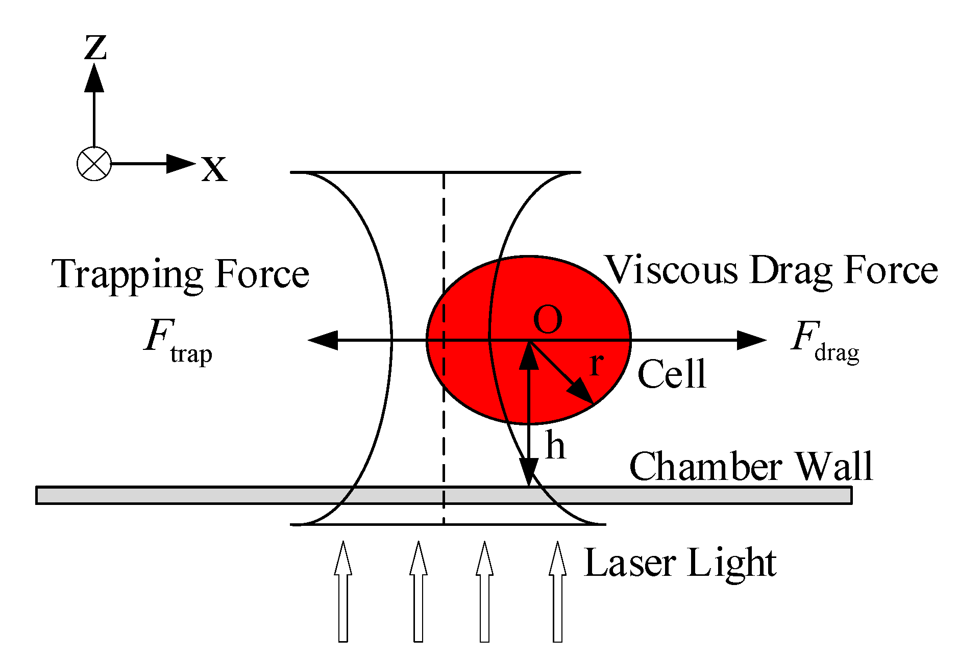
3.2. Cell Dynamics Model

The force on the X-Y axis of the cell is mainly composed of an optical trapping force and a viscous drag force from the liquid. In the Z-axis direction, the force acting on the cell includes the component of the optical trapping force in the Z-axis direction, the gravity acting on the cell and the buoyancy force. According to Newton’s third law, the force in the Z axis will be balanced when the cell is in a stable state. This section mainly studies the motion state of the cells captured by the optical trap under the force on the plane of the X-Y axis, and the force on the cells in the Z-axis direction does not contribute to the motion on the X-Y axis plane [39]. Thus, the force in the Z-axis direction is ignored. The force analysis of the cells in the optical trap is shown in Figure 3, and the force on the cell can be expressed by Equation (28).

$$m \ddot{\mathit{q}}=F_{\mathrm{trap}}-F_{\mathrm{drag}}$$

(28)

Because of the Reynolds number Re < < 1, the inertia force can be ignored [39]. Therefore, Equation (28) can be simplified as:

$$0=F_{\mathrm{trap}}-F_{\mathrm{drag}}$$

(29)

$$F_{\mathrm{trap}}=k\left(\mathit{l}\mathbf{-}\mathit{q}\right),\Vert \mathit{l}\mathbf{-}\mathit{q}\Vert \le r_0$$

(30)

$$F_{\mathrm{drag}}=\delta \dot{\mathit{q}}$$

(31)

where $F_{\mathrm{trap}}$ is the optical trapping force, $F_{\mathrm{drag}}$ is the blocking force, $k$ is the optical trap stiffness, $\mathit{l}\in {\mathsf{R}}^{2\times 1}$ is the position of the optical trap produced by optical tweezers, $\mathit{q}=\left[q_x;q_y\right]\in {\mathsf{R}}^{2\times 1}$ is the position of the cell, $\Vert \mathit{l}\mathbf{-}\mathit{q}\Vert$ is the offset between the center of the cell and the center of the optical trap, and $\delta$ is the coefficient of viscous resistance.

Substituting Equations (30) and (31) into Equation (29), the dynamic equation of the cell in the optical trap is obtained as:

$$0=k\left(\mathit{l}\mathbf{-}\mathit{q}\right)-\delta \dot{\mathit{q}},\Vert \mathit{l}\mathbf{-}\mathit{q}\Vert \le r_0$$

(32)

Rewriting Equation (32) as:

$$\frac{\delta }{k}\dot{\mathit{q}}=\mathit{l}\mathbf{-}\mathit{q},\Vert \mathit{l}\mathbf{-}\mathit{q}\Vert \le r_0$$

(33)

However, in practice, the micromanipulation of cells is very sensitive to environmental disturbances, such as stochastic dynamics caused by equipment vibration, liquid flow and random Brownian motion [40]. The interference term is recorded as $\mathit{d}\in {\mathsf{R}}^{2\times 1}$ and substituted into Equation (33). The actual cell dynamics model is shown as Equation (34):

$$\dot{\mathit{q}}=\frac{k}{\delta }\times (\mathit{l}\mathbf{-}\mathit{q})+\mathit{d},\Vert \mathit{l}\mathbf{-}\mathit{q}\Vert \le r_0$$

(34)

It should be noted that when the force on the cell is in equilibrium, the center of the cell is completely coincident with the center of the optical trap, and the optical trapping force is zero. The optical trapping force increases linearly with the offset between the cell center and the optical trap center until the offset is greater than $r_0$. When the offset is greater than $r_0$, the optical trapping force decreases with the increase of the offset. When the cell is completely outside the optical trap, the optical trapping force becomes zero. Therefore, in the process of manipulating cells with optical tweezers, the displacement of cells is usually constrained within the range of $r_0$.

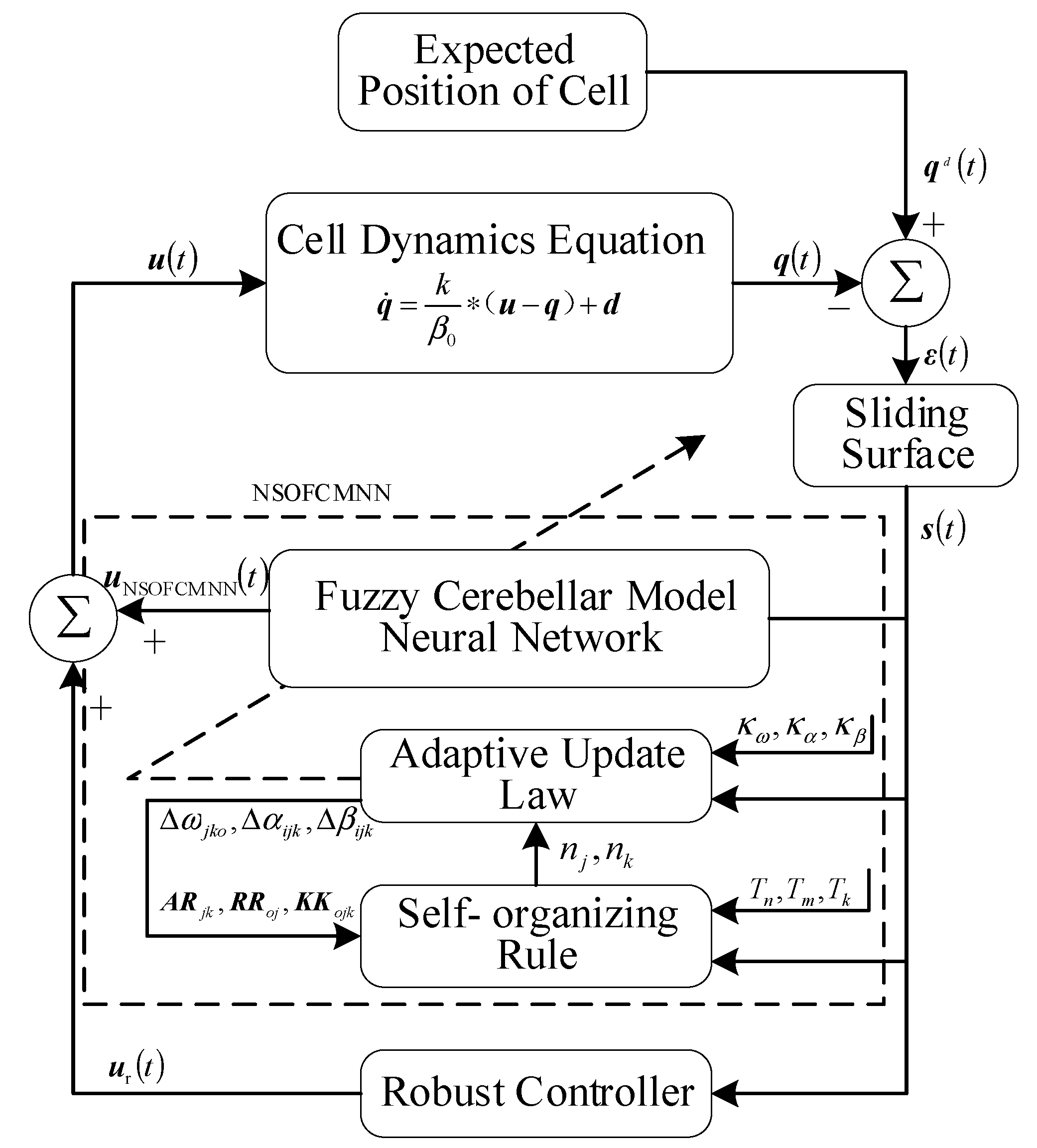
3.3. Cell Manipulation Control System

NSOFCMNN has strong learning and generalization ability for nonlinear mapping. It is used as the main controller of a control system, a robust compensator is added for eliminating approximation errors, and a higher order sliding surface is used to further weaken the influence of the external disturbances and the chattering on the system. Thus, the basic structure of the optical trap position manipulation control system is built.

Firstly, $\epsilon \left(t\right)$ is defined as an error:

$$\mathit{\epsilon }\left(t\right)={\mathit{q}}^{\mathit{d}}\left(t\right)-\mathit{q}\left(t\right)={\left[{\epsilon }_x\left(t\right),{\epsilon }_y\left(t\right)\right]}^T$$

(35)

where ${\mathit{q}}^d$ is the expected position of the cell and $\mathit{q}$ is the actual position of the cell. ${\epsilon }_x\left(t\right)$ is the error on the X-axis, ${\epsilon }_y\left(t\right)$ is the error on the Y-axis, and the sliding mode plane is introduced to represent another error function.

$$\mathit{s}\left(\epsilon ,t\right)=\mathit{\epsilon }{\left(t\right)}^{\prime }+K\mathit{\epsilon }\left(t\right)$$

(36)

where $\mathbf{K}$ is a matrix of constants and $\mathit{s}\left(\epsilon ,t\right)$ is a sliding mode vector.

In the practical application of cell manipulation control, some uncontrollable unknown factors will inevitably appear in the process of control, which is unavoidable in the control system, that is, the uncertainty in the cell dynamics. If the uncertainty term $\mathbf{L}$ is known, the ideal neural network controller is defined as:

$${\mathit{u}}_{\mathrm{NSOFCMNN}}^{\ast }\left(t\right)=\frac{\delta }{k}\ast \left(\mathit{q}\left(t-1\right)-{\dot{\mathit{q}}}^{\mathit{d}}\left(t\right)\right)+\mathit{q}\left(t-1\right)-\mathit{d}$$

(37)

$$\mathit{d}={\mathit{d}}_{\mathrm{NSOFCMNN}}\left(X, {\alpha }_{ijk}, {\beta }_{ijk}, {\omega }_{jko}, {\psi }_{jk}\right)+\mathit{\sigma }$$

(38)

where $\mathit{\sigma }={\left[{\sigma }_1,{\sigma }_2\right]}^T$ is the error between the ideal neural network controller and the actual manipulation controller. This approximation error is assumed to be bounded and satisfy $0\le \Vert {\sigma }_1\Vert \le N_1$, $0\le \Vert {\sigma }_2\Vert \le N_2$, $\mathit{N}={\left[N_1,N_2\right]}^T$, $\Vert \cdot \Vert$ represents the norm.

An approximate error bound $\mathit{N}$ is assumed; however, it is difficult to measure in practical applications. Therefore, a bound estimate is set to estimate this bound error. The estimated error for the bounds is defined as follows:

$$\tilde{\mathit{N}}=\mathit{N}-\widehat{\mathit{N}}$$

(39)

where $\widehat{\mathit{N}}$ is an estimate of $\mathit{N}$, and the robust controller aims to compensate for the effects of approximation errors, expressed as:

$${\mathit{u}}_{\mathit{r}}=\widehat{\mathit{N}}\tanh (\mathit{s})$$

(40)

Combining the NSOFCMNN controller with a robust compensator, an optical trap position manipulation control system is finally built.

$$\mathit{u}={\mathit{u}}_{\mathrm{NSOFCMNN}}+{\mathit{u}}_r$$

(41)

The structure of the cell manipulation control system is shown in Figure 4:

After the error $\epsilon \left(t\right)$ between the expected position ${\mathit{q}}^d$ and the actual position $\mathit{q}$ of the cell passes through the sliding mode surface, $\mathit{s}\left(t\right)$ is used as the input data of NSOFCMNN, and its output plus the output of the robust compensator constitutes the total output of the control system. The holographic optical tweezers system finally realizes the manipulation of biological cells by generating several optical traps at specific expected positions at each time point according to the number of cells to be controlled and the total output of the control system.

In the practical application of holographic optical tweezers, the maximum moving distance of the optical trap needs to be limited. When $\mathit{u}\le \left(\mathit{q}\pm {[r_0,r_0]}^T\right)$ and $\Vert \mathit{l}\mathbf{-}\mathit{q}\Vert \le r_0$ are satisfied at the same time, the position movement range of the output optical trap is limited. Such a control design ensures that the deviation of the cell from the trap is within the range $\left[-r_0,r_0\right]$, and the cell does not escape from the trap. At this point it is no longer necessary to discuss the situation in which the cells are detached from the optical trap when $\Vert \mathit{l}\mathbf{-}\mathit{q}\Vert >r_0$.

In the study of multicellular cooperative control, by extending Equation (33), the dynamics of the $i$th trapped cell is expressed as:

$$\frac{{\delta }_i}{k_i}{\dot{\mathit{q}}}_i={\mathit{l}}_i-{\mathit{q}}_i,\Vert {\mathit{l}}_i-{\mathit{q}}_i\Vert \le r_0,i=1,2,\dots n$$

(42)

where ${\mathit{q}}_i$, ${\delta }_i$ and $k_i$ represent the ith cell position, optical trap stiffness and viscous drag coefficient, respectively. ${\mathit{l}}_i$ represents the position of the $i$th optical trap generated by the holographic optical tweezers.

In order to avoid collisions between multiple cells, and to achieve complex multi-cellular cooperative control tasks at the same time, a virtual cell is set, and the error between the cell and the expected position can still refer to Equation (35). All other controlled cells are spaced a certain distance from the virtual cells:

$${\mathit{\tau }}_i\left(t\right)={\mathit{q}}_0\left(t\right)-{\mathit{q}}_i\left(t\right)$$

(43)

where ${\mathit{\tau }}_i\in {{R}}^{2\times 1}$ is the expected relative spacing between the ith controlled cell and the virtual cell in the X-axis and Y-axis directions, and ${\mathit{q}}_0$ is the position of the virtual cell. Combining Equations (35) and (43), the error between the position of each controlled cell and the expected position is expressed as Equation (44), and when $t\to \infty$, ${\mathit{\epsilon }}_i\left(t\right)\to 0$, it can be satisfied that each cell maintains a certain distance and realizes multi-cell coordinated control.

$${\mathit{\epsilon }}_i\left(t\right)={\mathit{q}}^d\left(t\right)-{\mathit{q}}_i\left(t\right)-{\mathit{\tau }}_i\left(t\right)$$

(44)

In addition, the uncertain interference term $\mathit{d}$ existing in the actual movement process of the cell can be updated, together with $\mathit{\epsilon }$ in the neural network learning.

3.4. Lyapunov Convergence Analysis

The learning rates ${\kappa }_{\omega },{\kappa }_{\alpha },{\kappa }_{\beta }$ in formulas (7), (9), and (10) need to be selected correctly. A smaller learning rate can ensure the convergence of NSOFCMNN parameters in the controller, but the learning speed is slower. On the other hand, if a large learning rate is chosen, it may cause the learning to diverge. In order to satisfy the stable convergence of the parameters, the convergence is analyzed below, and the range of the specific learning rate is derived.

We defined ${\mathit{\Gamma }}_{\mathit{\gamma }}\left(t\right)=\mathit{\partial }{u}_{NSOFC{M}_o}/\mathit{\partial }\mathit{\gamma }=\mathit{\partial }{O}_o/\mathit{\partial }\mathit{\gamma }$, for $\mathit{\gamma }=\mathit{\omega },\mathit{\alpha },\mathit{\beta }$, which can be calculated as:

$$\begin{array}{l}\mathit{\Gamma }\mathit{\omega }\left(t\right)=\frac{\mathit{\partial }{O}_o}{\mathit{\partial }\mathit{\omega }}\\ \hspace{1em}\hspace{1em}\hspace{1em}={\left[\frac{\mathit{\partial }{O}_o}{\mathit{\partial }{\omega }_{jk1}},\dots ,\frac{\mathit{\partial }{O}_o}{\mathit{\partial }{\omega }_{jko}},\dots ,\frac{\mathit{\partial }{O}_o}{\mathit{\partial }{\omega }_{jk{n}_o}}\right]}^T\end{array}$$

(45)

$$\begin{array}{l}\frac{\mathit{\partial }{O}_o}{\mathit{\partial }{\omega }_{jko}}=\left[\frac{\mathit{\partial }{O}_o}{\mathit{\partial }{\omega }_{11o}}\right.,\dots ,\frac{\mathit{\partial }{O}_o}{\mathit{\partial }{\omega }_{1n_{k}o}},\frac{\mathit{\partial }{O}_o}{\mathit{\partial }{\omega }_{21o}},\\ \hspace{1em}\hspace{1em}=\left.\dots ,\frac{\mathit{\partial }{O}_o}{\mathit{\partial }{\omega }_{2n_{k}o}},\dots ,\frac{\mathit{\partial }{O}_o}{\mathit{\partial }{\omega }_{n_{j}1o}},\dots ,\frac{\mathit{\partial }{O}_o}{\mathit{\partial }{\omega }_{n_j{n}_{k}o}}\right]\end{array}$$

(46)

$$\begin{array}{l}\mathit{\Gamma }\mathit{\alpha }\left(t\right)=\frac{\mathit{\partial }{O}_o}{\mathit{\partial }\mathit{\alpha }}\\ \hspace{1em}\hspace{1em}\hspace{1em}={\left[\frac{\mathit{\partial }{O}_o}{\mathit{\partial }{\alpha }_{1jk}},\dots ,\frac{\mathit{\partial }{O}_o}{\mathit{\partial }{\alpha }_{ijk}},\dots ,\frac{\mathit{\partial }{O}_o}{\mathit{\partial }{\alpha }_{n_{i}jk}}\right]}^T\end{array}$$

(47)

$$\begin{array}{l}\frac{\mathit{\partial }{O}_o}{\mathit{\partial }{\alpha }_{ijk}}=\left[\frac{\mathit{\partial }{O}_o}{\mathit{\partial }{\alpha }_{i11}}\right.,\dots ,\frac{\mathit{\partial }{O}_o}{\mathit{\partial }{\alpha }_{i1n_k}},\frac{\mathit{\partial }{O}_o}{\mathit{\partial }{\alpha }_{i21}},\\ \hspace{1em}\hspace{1em}=\left.\dots ,\frac{\mathit{\partial }{O}_o}{\mathit{\partial }{\alpha }_{i2n_k}},\dots ,\frac{\mathit{\partial }{O}_o}{\mathit{\partial }{\alpha }_{i{n}_{j}1}},\dots ,\frac{\mathit{\partial }{O}_o}{\mathit{\partial }{\alpha }_{i{n}_j{n}_k}}\right]\end{array}$$

(48)

$$\begin{array}{l}\mathit{\Gamma }\mathit{\beta }\left(t\right)=\frac{\mathit{\partial }{O}_o}{\mathit{\partial }\mathit{\beta }}\\ \hspace{1em}\hspace{1em}\hspace{1em}={\left[\frac{\mathit{\partial }{O}_o}{\mathit{\partial }{\beta }_{1jk}},\dots ,\frac{\mathit{\partial }{O}_o}{\mathit{\partial }{\beta }_{ijk}},\dots ,\frac{\mathit{\partial }{O}_o}{\mathit{\partial }{\beta }_{n_{i}jk}}\right]}^T\end{array}$$

(49)

$$\begin{array}{l}\frac{\mathit{\partial }{O}_o}{\mathit{\partial }{\alpha }_{ijk}}=\left[\frac{\mathit{\partial }{O}_o}{\mathit{\partial }{\alpha }_{i11}}\right.,\dots ,\frac{\mathit{\partial }{O}_o}{\mathit{\partial }{\alpha }_{i1n_k}},\frac{\mathit{\partial }{O}_o}{\mathit{\partial }{\alpha }_{i21}},\\ \hspace{1em}\hspace{1em}=\left.\dots ,\frac{\mathit{\partial }{O}_o}{\mathit{\partial }{\alpha }_{i2n_k}},\dots ,\frac{\mathit{\partial }{O}_o}{\mathit{\partial }{\alpha }_{i{n}_{j}1}},\dots ,\frac{\mathit{\partial }{O}_o}{\mathit{\partial }{\alpha }_{i{n}_j{n}_k}}\right]\end{array}$$

(50)

The Lyapunov function is defined as:

$$\mathit{L}\left(t\right)=\mathit{\epsilon }{\left(t\right)}^T\mathit{\epsilon }\left(t\right)$$

(51)

where

$$\begin{array}{l}\mathit{\epsilon }\left(t\right)=\left[{\epsilon }_1\left(t\right),\dots ,{\epsilon }_o\left(t\right),\dots ,{\epsilon }_{n_o}\left(t\right)\right]\\ \hspace{1em}\hspace{1em}=\left[O\right.d_1\left(t\right)-O_1\left(t\right),\dots ,O{d}_o\left(t\right)-O_o\left(t\right),\\ \hspace{1em}\hspace{1em}\left.\dots ,O{d}_{n_o}\left(t\right)-O_{n_o}\left(t\right)\right]\end{array}$$

(52)

The change of the Lyapunov function is:

$$\begin{array}{l}\mathsf{\Delta }\mathit{L}\left(t\right)=\mathit{L}\left(t+1\right)-\mathit{L}\left(t\right)\\ =\mathit{\epsilon }{\left(t+1\right)}^T\mathit{\epsilon }\left(t+1\right)-\mathit{\epsilon }{\left(t\right)}^T\mathit{\epsilon }\left(t\right)\\ ={\left[\mathit{\epsilon }\left(t+1\right)+\mathit{\epsilon }\left(t\right)\right]}^T\left[\mathit{\epsilon }\left(t+1\right)-\mathit{\epsilon }\left(t\right)\right]\\ ={\left[2\mathit{\epsilon }\left(t\right)+\mathsf{\Delta }\mathit{\epsilon }\left(t\right)\right]}^T\mathsf{\Delta }\mathit{\epsilon }\left(t\right)\end{array}$$

(53)

According to Taylor’s formula, the error is written as:

$$\begin{array}{cc}\hfill \mathit{\epsilon }\left(t+1\right)& =\mathit{\epsilon }\left(t\right)+\mathsf{\Delta }\mathit{\epsilon }\left(t\right)\hfill \\ \hfill \hspace{1em}& \cong \mathit{\epsilon }\left(t\right)+\left[\frac{\mathit{\partial }\mathit{\epsilon }\left(t\right)}{\mathit{\partial }\mathit{\gamma }}\right]\mathsf{\Delta }\mathit{\gamma }\hfill \end{array}$$

(54)

Using the chain rule, and similarly to formulas (7), (9) and (10), as the following is obtained:

$$\frac{\mathit{\partial }\mathit{\epsilon }\left(t\right)}{\mathit{\partial }\mathit{\gamma }}=\frac{\mathit{\partial }\epsilon \left(t\right)}{\mathit{\partial }{O}_o\left(t\right)}\frac{\mathit{\partial }{O}_o\left(t\right)}{\mathit{\partial }\mathit{\gamma }}=-{\mathit{\Gamma }}_{\gamma }\left(t\right)$$

(55)

$$\mathsf{\Delta }\mathit{\gamma }=-\kappa \frac{\mathit{\partial }E\left(t\right)}{\mathit{\partial }\mathit{\gamma }}=-\kappa \frac{\mathit{\partial }E\left(t\right)}{\mathit{\partial }{O}_o\left(t\right)}\frac{\mathit{\partial }{O}_o\left(t\right)}{\mathit{\partial }\mathit{\gamma }}=\kappa \mathit{\epsilon }\left(t\right){\mathit{\Gamma }}_{\gamma }\left(t\right)$$

(56)

From Equations (53) to (56), $\mathsf{\Delta }L\left(t\right)$ can be obtained as:

$$\begin{array}{cc}\hfill \mathsf{\Delta }\mathit{L}\left(t\right)& ={\left[2\mathit{\epsilon }\left(t\right)+\mathsf{\Delta }\mathit{\epsilon }\left(t\right)\right]}^T\mathsf{\Delta }\mathit{\epsilon }\left(t\right)\hfill \\ \hfill & =-\kappa \mathit{\epsilon }{\left(t\right)}^T\mathit{\epsilon }\left(t\right)P\left(2-\kappa P\right)\hfill \end{array}$$

(57)

where $P={\left[\frac{\mathit{\partial }{O}_o\left(t\right)}{\mathit{\partial }\mathit{\gamma }}\right]}^T\left[\frac{\mathit{\partial }{O}_o\left(t\right)}{\mathit{\partial }\mathit{\gamma }}\right]$.

In Equation (56), $\kappa$ is the learning rate of NSOFCMNN, which represents ${\kappa }_{\alpha }$, ${\kappa }_{\beta }$ or ${\kappa }_{\omega }$. To ensure stable convergence, $\kappa$ needs to be selected in the following range:

$$0<\kappa <\frac{2}{(\left[\frac{\mathit{\partial }{O}_o\left(t\right)}{\mathit{\partial }\mathit{\gamma }}{]}^T\left[\frac{\mathit{\partial }{O}_o\left(t\right)}{\mathit{\partial }\mathit{\gamma }}\right]\right)}$$

(58)

When $\kappa$ is selected as Equation (58), $\mathsf{\Delta }\mathit{L}\left(t\right)$ in Equation (57) is always less than 0. The Lyapunov stability conditions $\mathit{L}\left(t\right)>0$ and $\mathsf{\Delta }\mathit{L}\left(t\right)<0$ are satisfied, and the error convergence can be guaranteed at this time.

4. Simulation Results

The holographic optical tweezers system can obtain the position information of all cells from the image information [41], and each optical trap can be placed anywhere in the focal length of the objective lens. Multi-cell cooperative control can be realized by placing the optical trap in an ideal position. In order to prove the effectiveness and advantages of the control system of optical tweezers based on the novel NSOFCMNN proposed in this paper, MATLAB simulation experiments were carried out on single-cell control and multi-cell control, respectively.

Firstly, we make the following assumptions:

Hypothesis 1.

There is no delay in obtaining information from real-time image position of cells.

Hypothesis 2.

In the holographic optical tweezers system, the optical trap is placed without delay.

Hypothesis 3.

Controlled cell size, volume, weight, etc., are exactly the same.

Both single-cell and multi-cell manipulation simulation experiments take the transport of yeast cells as example [16].

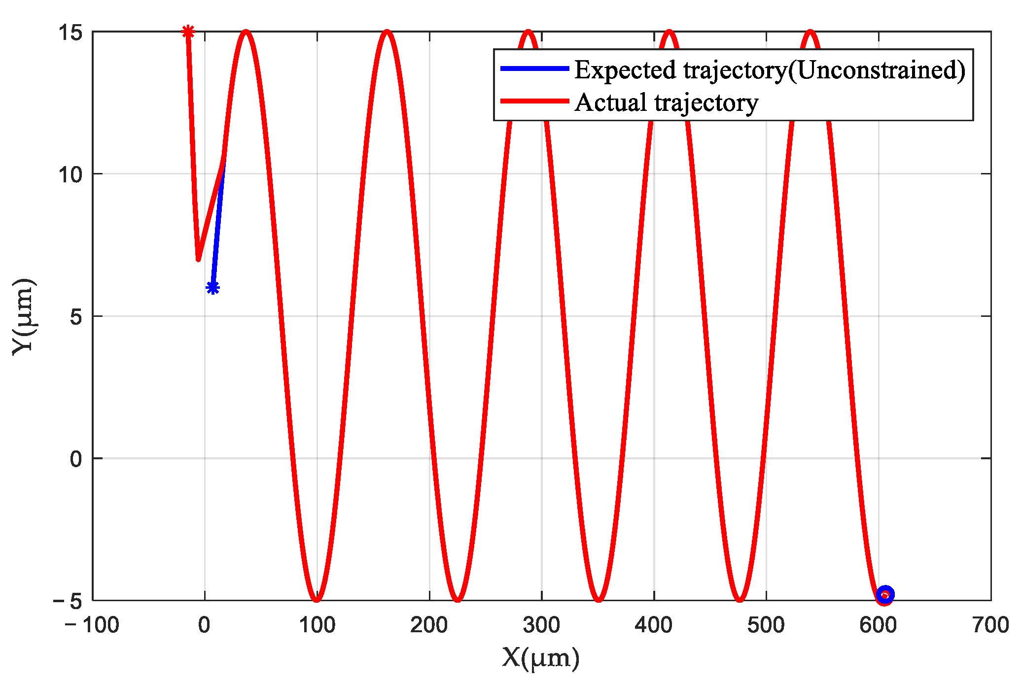
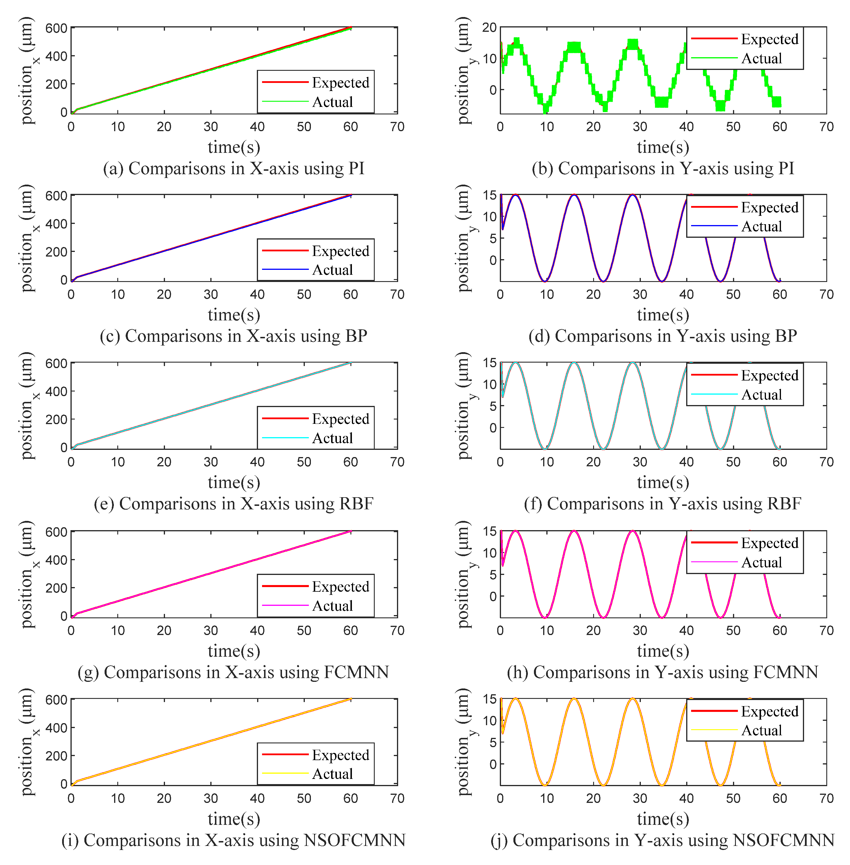
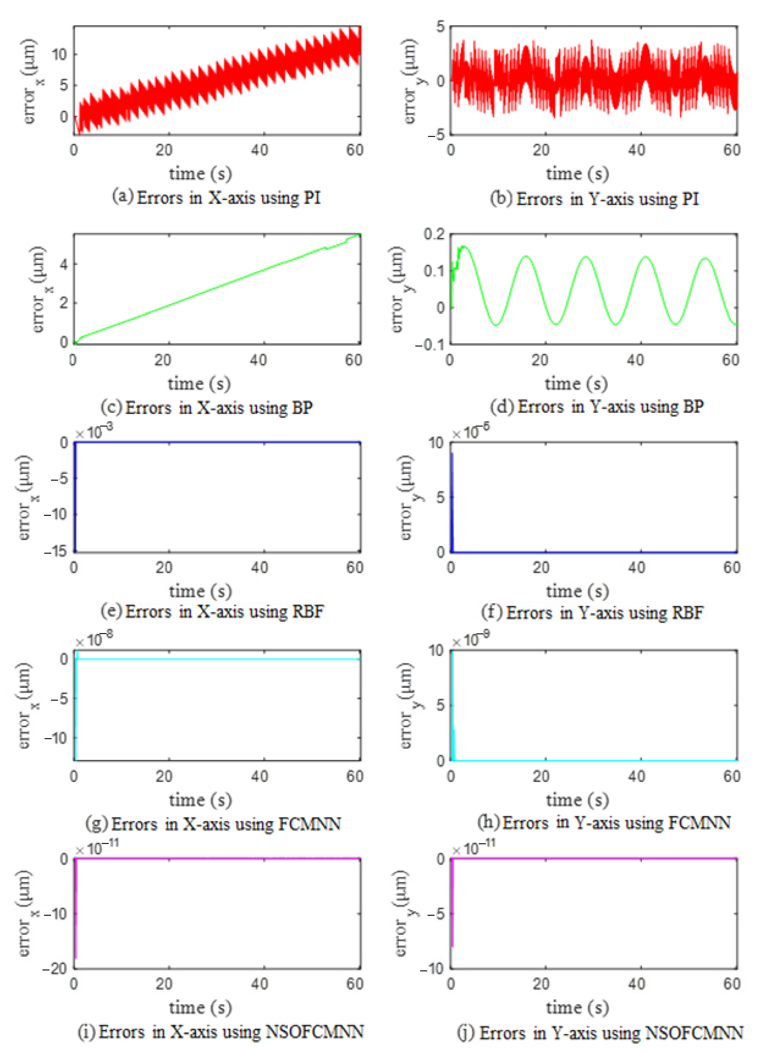
4.1. Case (1): Holographic Optical Tweezers Manipulate Control for Single Cells

The size of the yeast is set as 6 μm, the initial position is [–15, 15], It can be seen from

Table 1. Relationship between cell velocity and kinetic coefficient.

Cell Velocity (μm/s)	±5	±7.5	±10
$\delta /k\left(\mathrm{s}\right)$	0.09	0.1	0.09

that when the viscous resistance coefficient $\delta /k$ of the liquid environment is taken as 0.09, and the maximum moving speed is 10 μm/s 40. Because the cells are controlled by the optical trap, which is generated by the holographic optical tweezers system, the maximum moving speed of the output optical trap is also 10 μm/s, and the maximum moving distance of the optical trap is less than $r_0$.

In practical applications, there are often some obstacle cells and other obstacles in the environment where biological cells are located. A trajectory ${\mathit{q}}^d$ which satisfies the cells to reach the expected position without collision can be set in advance, such as the expected cell trajectory containing trigonometric functions [38,40], so that the biological cells can smoothly reach the expected position along the preset trajectory [12,42]. The expected trajectory ${\mathit{q}}^{d1}={\left[q_x{}^{d1},q_y{}^{d1}\right]}^T$ that satisfies the condition in a certain cell environment is set as Equations (59) and (60).

$$\left\{\begin{array}{cc}{q}_x{}^{d1}=5+t,& { \mathrm{if} -r}_x\le q_x{}^{d1}-q_x\le r_x\\ q_x{}^{d1}=q_x+r_x,& \mathrm{if} q_x{}^{d1}-q_x>r_x\\ q_x{}^{d1}=q_x-r_x,& \mathrm{if} q_x{}^{d1}-q_x<{-r}_x\end{array}\right.$$

(59)

$$\left\{\begin{array}{cc}{q}_y{}^{d1}=5+10\sin \left(0.05t\right)& { \mathrm{if} -r}_y\le q_y{}^{d1}-q_y\le r_y\\ q_y{}^{d1}=q_y+r_y,& \mathrm{if} q_y{}^{d1}-q_y>r_y\\ q_y{}^{d1}=q_y-r_y,& \mathrm{if} q_y{}^{d1}-q_y<{-r}_y\end{array}\right.$$

(60)

where $r_x$ and $r_{\mathrm{y}}$ are trajectory constraint parameters, which represent the maximum confinement offset between the center of the cell and the center of the optical trap on the X and Y axes, respectively, and satisfy $\Vert r_x,r_y\Vert =\Vert l-q\Vert \le r_0$.

Setting constraints on the desired trajectory can further ensure that the light trap will not leave the center of the cell within a certain range, and the cell can also quickly and effectively reach the desired position at the initial time. Because the maximum moving distance of the optical trap is limited, the trajectory error can also be minimized.

Considering the sensitivity of micromanipulation to environmental interference, the interference term $\mathit{d}={\left[d_x,d_y\right]}^T$ is set, where $d_x$ and $d_y$ are the interference terms in the X-axis direction and the Y-axis direction, respectively.

$$\left\{\begin{array}{c}{d}_x=0.5\sin \left(0.05t\right),\begin{array}{cc}& \end{array}0 \mathrm{s}\le t\le 5 \mathrm{s}\\ d_y=0.3\cos \left(0.03t\right),\begin{array}{cc}& \end{array}0 \mathrm{s}\le t\le 5 \mathrm{s}\end{array}\right.$$

(61)

In the simulation experiment in this section, the sampling time is set to 0.1 s, the simulation time $t_{max}=60 \mathrm{s}$, and the trajectory constraint parameter $r_x$=$r_{\mathrm{y}}=3$. In order to verify the control performance of the NSOFCMNN controller, the PI controller, BP neural network controller, RBF neural network controller and FCMNN controller are also used for comparison with the NSOFCMNN in this paper. The number of iterations of each neural network is set to 50, and the sliding surface parameter K = [0.3x₁,0.3x₂]^T. In the PI controller, $k_p$ = 20, $k_i$ = 0.5. The number of hidden layer nodes of the BP neural network is 3, the number of neurons of the RBF neural network is 3, the number of layers of the FCMNN is fixed to 3, and the number of blocks is fixed to 3. The initial number of layers and initial blocks of the NSOFCMNN are both 3, and the self-organizing structure adjustment parameter $T_n$ = 0.01, $T_m$= 0.0001, $T_k$= 0.32.

Figure 5 shows the comparison between the expected trajectory without constraints and the trajectory of a single cell manipulated by the optical trap which is generated by the holographic optical tweezers system when using NSOFCMNN as the main controller. Due to the addition of the trajectory constraint parameters $r_x$ and $r_y$, the controlled yeast cells will not be immediately moved to the unconstrained expected trajectory at the initial time, but will move along the constrained expected trajectory in Equations (59) and (60). It is ensured that the trajectory error is not affected by the maximum moving distance $r_0$ of the optical trap. As time goes by, the cell trajectories gradually coincided with the expected trajectories of the unconstrained conditions.

Figure 6 is a comparison between the actual trajectories and expected trajectories of cells when different neural networks are used as the main controller. It can be seen from Figure 6 that when the PI is used as the main controller, there is a large error in both the X-axis and Y-axis directions, and it cannot be well applied in the single-cell manipulation control. When the BP, the RBF, the FCMNN or the NSOFCMNN is used as the main controllers, it has great advantages over the PI main controller in the trajectory tracking of single-cell manipulation control.

Figure 7 shows the trajectory error using different neural networks as the main controller when holographic optical tweezers manipulate single cells. It can be seen more clearly from Figure 7 that the manipulation control error of the latter three neural networks as the main controller is obviously closer to 0.

In order to further compare the control effect between the proposed NSOFCMNN and other controllers, the method of calculating RMSE and MAE to compare the specific errors between them was used, and the corresponding formulas of the two errors are Equations (62) and (63), respectively.

$$RMSE=\sqrt{{\displaystyle \sum _{t=0}^{t_{\max }}{\left(q^d\left(t\right)-q\left(t\right)\right)}^2/\left(t_{\max }+1\right)}}$$

(62)

$$MAE={\displaystyle \sum }_{t=0}^{t_{\max }}\left|q^d\left(t\right)-q\left(t\right)\right|/\left(t_{\max }+1\right)$$

(63)

According to Equations (62) and (63),

Table 2. Root mean square error (RMSE) and mean absolute error (MAE) of single-cell manipulation.

Data Type	Main Controller	X-Axis	Y-Axis
RMSE of single-cell manipulation	PI	7.0 × 10−6	1.8 × 10−6
	BP	3.2 × 10−6	8.4 × 10−8
	RBF	6.2 × 10−10	4.0 × 10−12
	FCMNN	5.3 × 10−15	4.2 × 10−16
	This work	7.4 × 10−18	3.3 × 10−18
MAE of single-cell manipulation	PI	5.5 × 10−5	3.7 × 10−6
	BP	1.3 × 10−5	5.8 × 10−8
	RBF	2.5 × 10−11	2.1 × 10−13
	FCMNN	2.0 × 10−16	2.1 × 10−17
	This work	3.0 × 10−19	1.3 × 10−19

is obtained. Among these two kinds of errors, RMSE can evaluate the degree of error using different controllers, and MAE can better reflect the actual situation of the error.

The RMSE and MAE of single-cell manipulation for different main controllers are shown in Table 2. It can be seen that when FCMNN is used as the main controller, RMSE and MAE only float up and down 5.0 × 10⁻¹⁵ and 2.0 × 10⁻¹⁶, respectively, which are smaller than the RMSE and MAE when PI, BP and RBF are used as the main controllers, respectively, and the control accuracy is relatively high. Compared with the FCMNN main controller, the RMSE and MAE of the proposed NSOFCMNN are only 0.1–1% of the former. It can be concluded that the single-cell manipulation control of the NSOFCMNN main controller has better control performance than the other main controller, and even in the presence of interference factors, it can also have better robustness.

Figure 8 shows the changes in the number of layers and blocks of the NSOFCMNN proposed in this paper during the manipulation of single cells by holographic optical tweezers. Due to the large error between the actual position of the cell and the expected position at the beginning, the number of layers and blocks of NSOFCMNN are adjusted from three layers and three blocks to seven layers and four blocks. When the error continues to converge, the number of network layers is reduced to four layers, and the number of blocks is reduced to two layers, which improves the learning efficiency of the proposed NSOFCMNN until the end of the simulation experiment. The simulation results in this section also demonstrate that the proposed NSOFCMNN can effectively adjust the network structure in real time according to the input data.

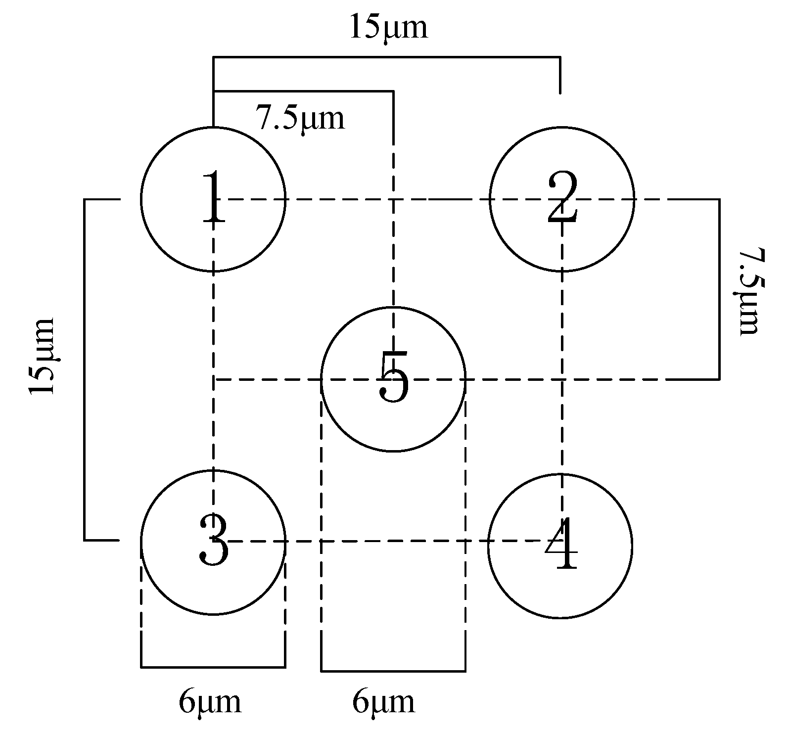
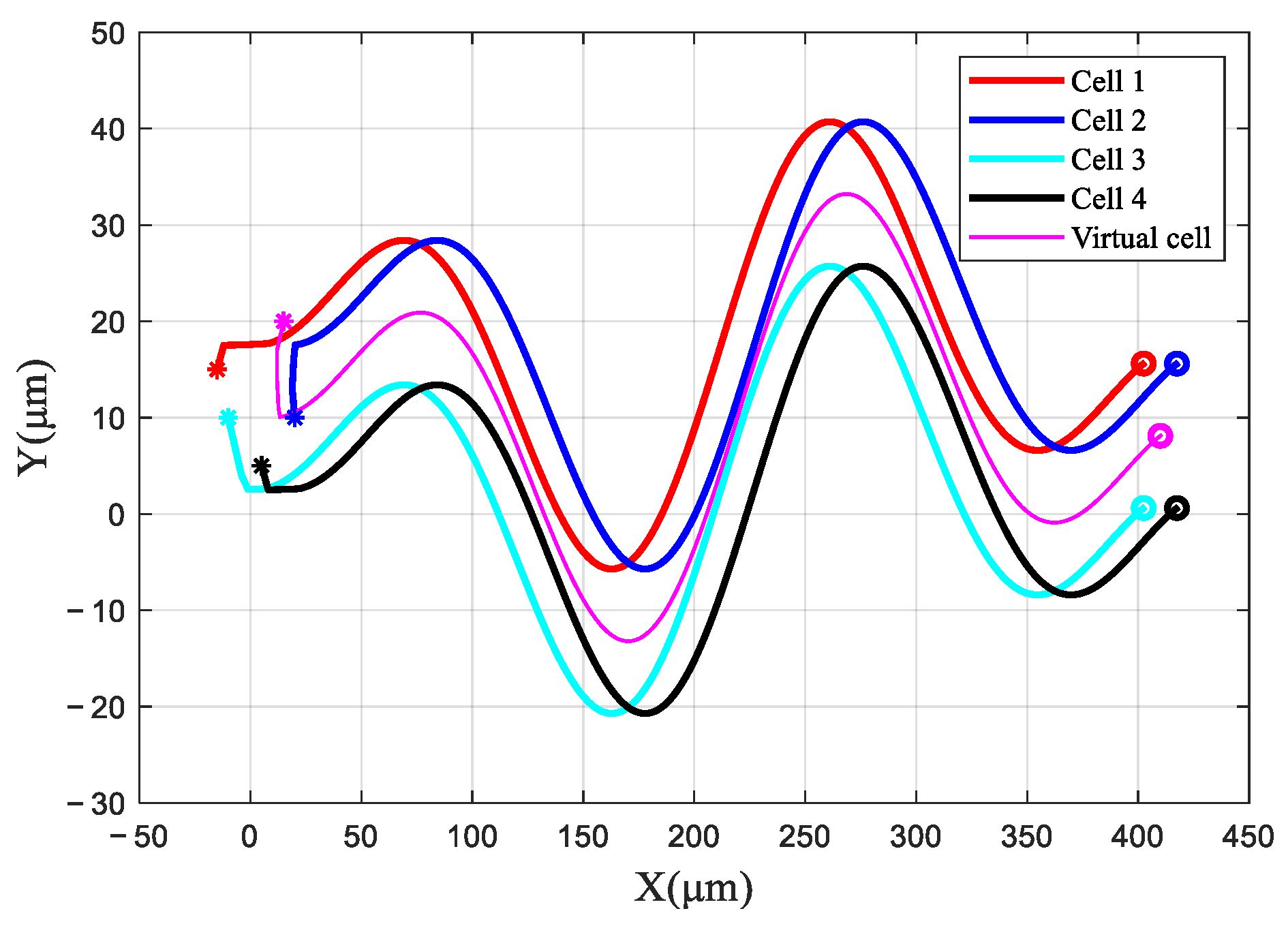
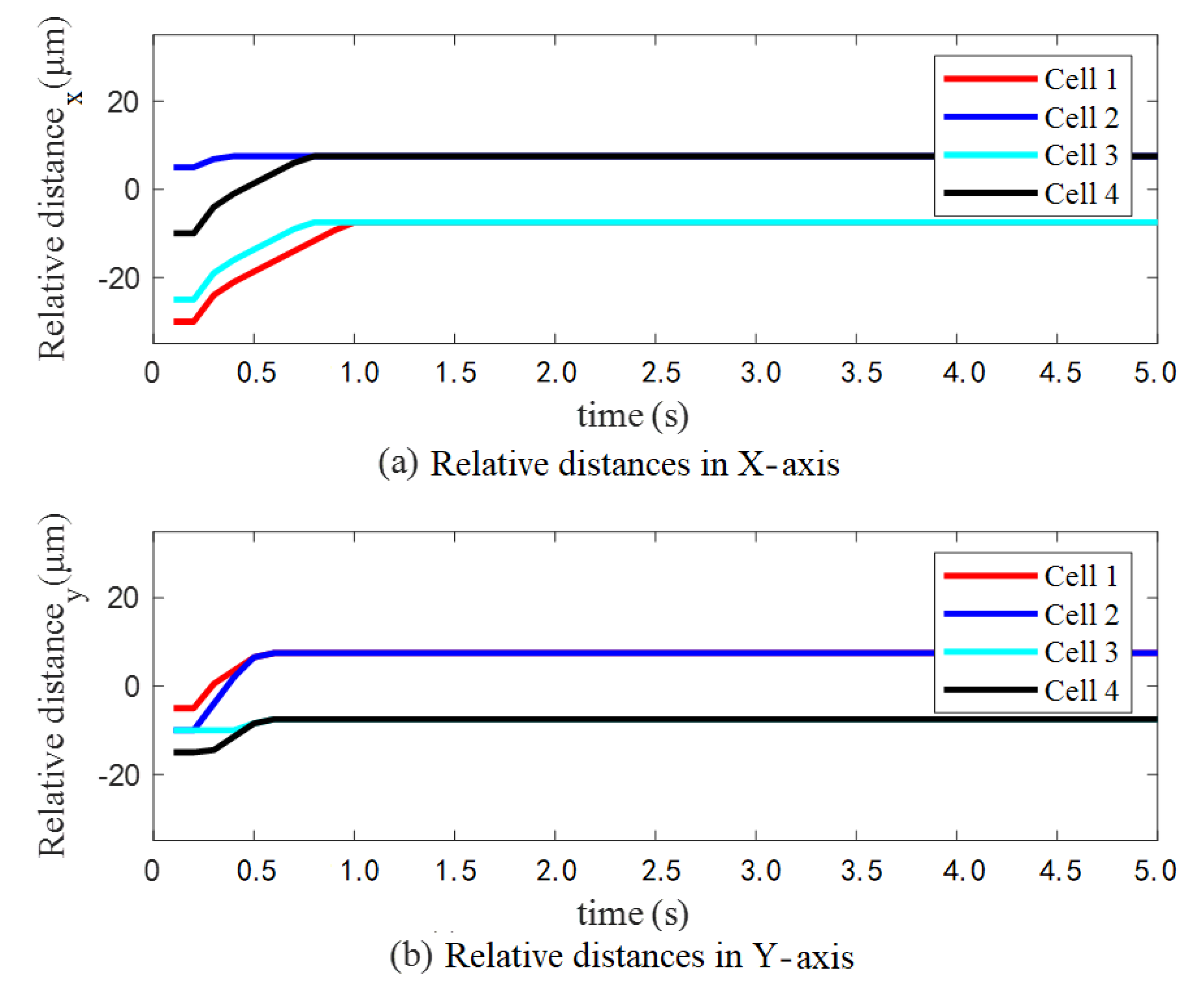
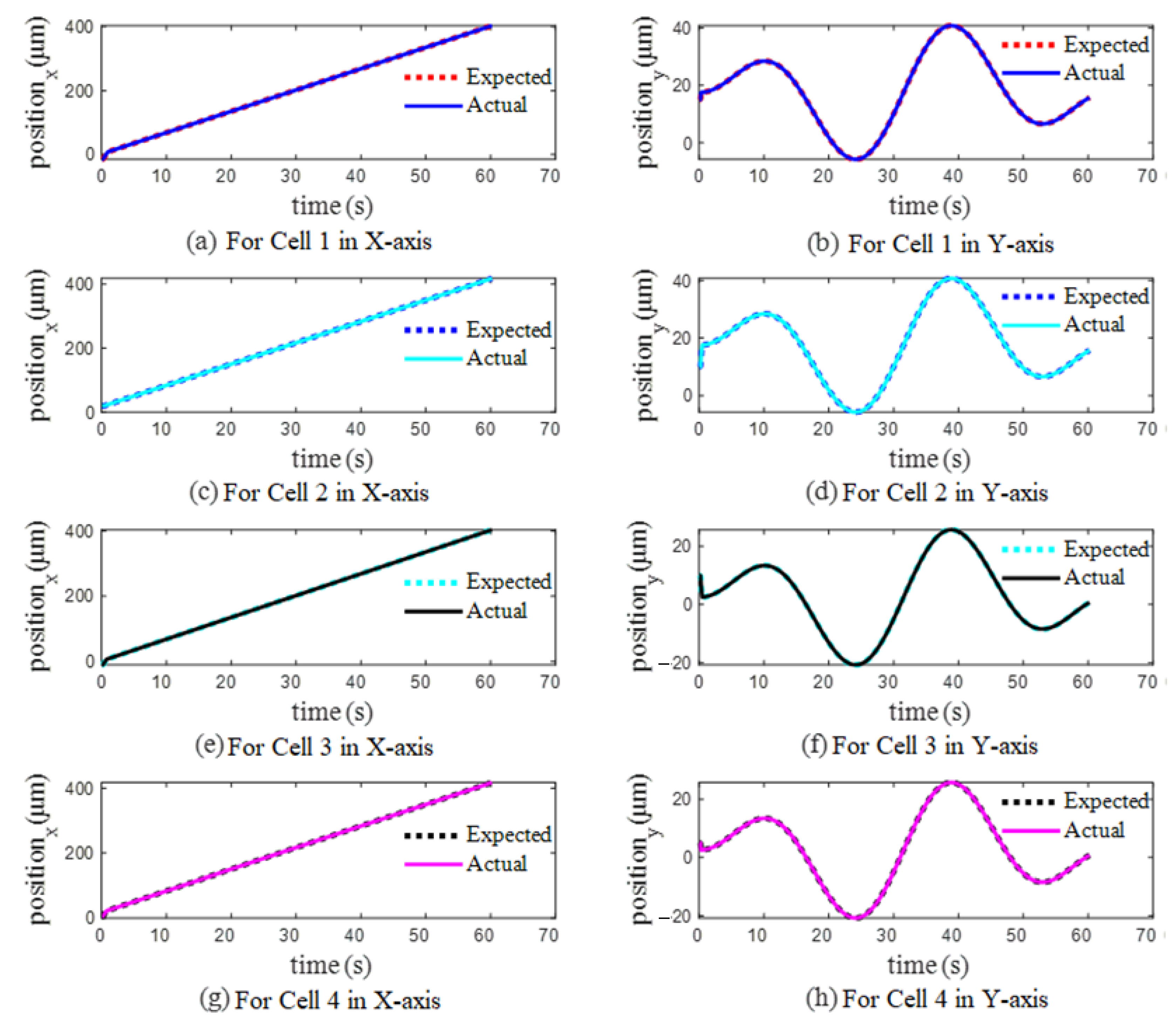
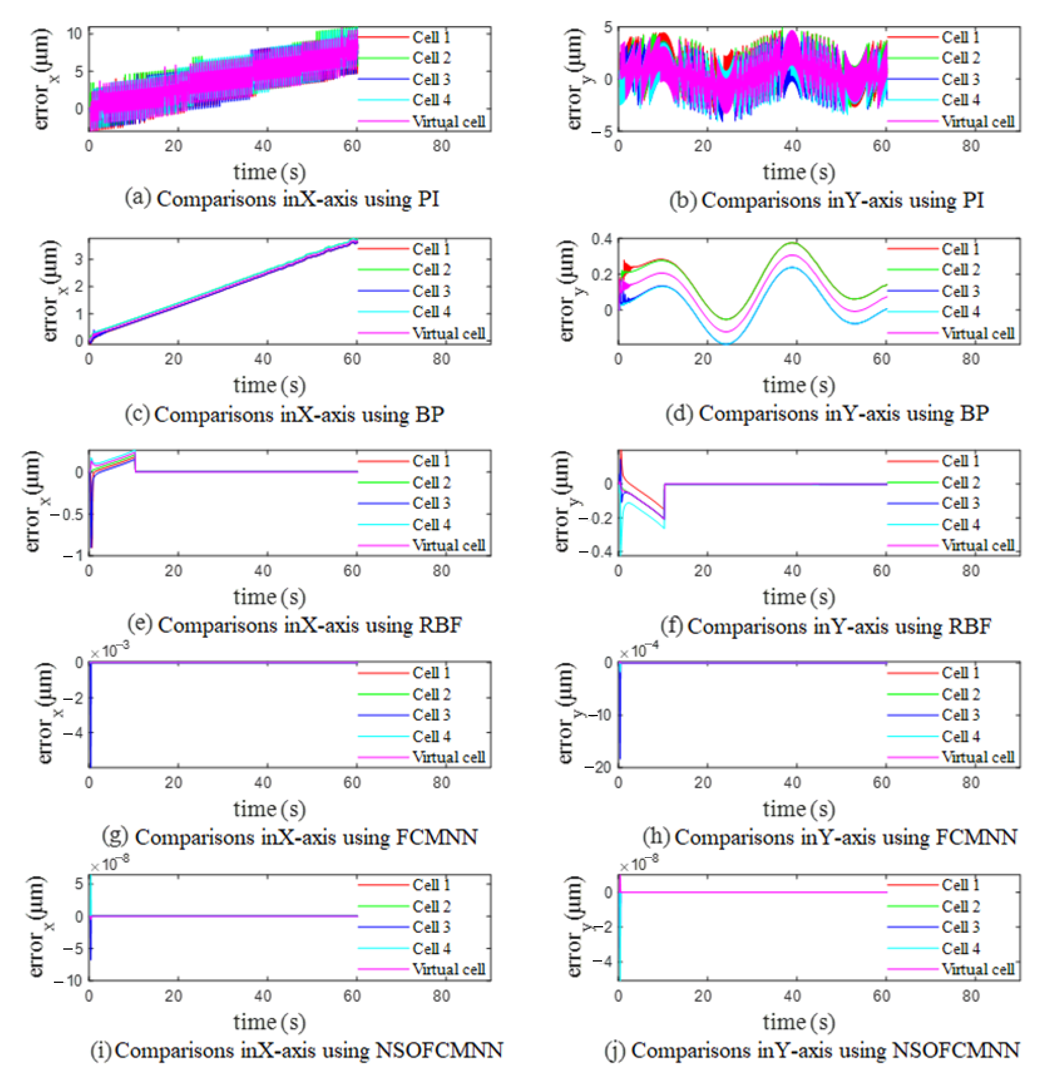
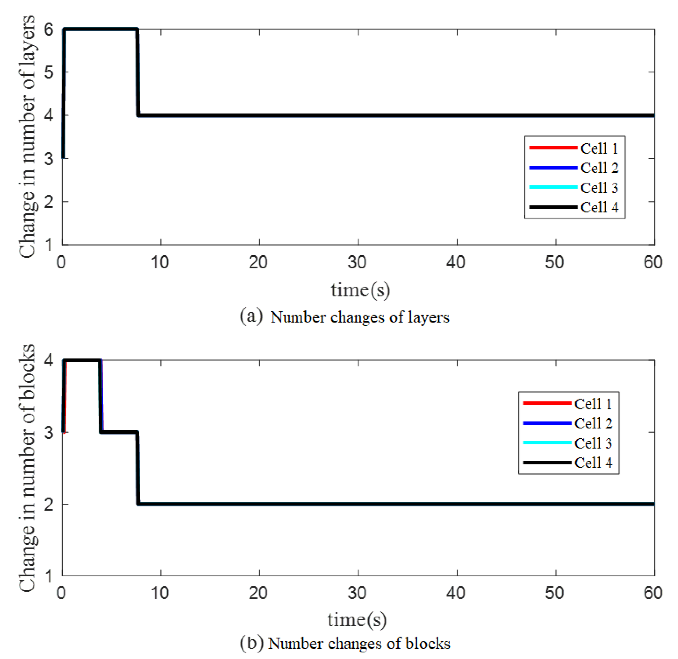
4.2. Case (2): Holographic Optical Tweezers Manipulate Control for Multiple Cells

Similar to Case (1) described in Section 4.1, it is assumed that there are four yeast cells in another cell environment, and the expected trajectory ${\mathit{q}}^{d2}={\left[q_x{}^{d2},q_y{}^{d2}\right]}^T$ that satisfies the multi-cell collision-free arrival at the expected position is given by Equation (64).

$$\left\{\begin{array}{c}{q}_x{}^{d2}=10+\frac{2}{3}t\\ q_y{}^{d2}=10+5\sin \left(0.05t\right)\sin \left(0.02t\right)\end{array}\right.$$

(64)

The initial position of each yeast cell is shown in

Table 3. Initial position of each yeast cell.

	Cell 1	Cell 2	Cell 3	Cell 4	Virtual Cell
initial position (μm)	[−15, 15]	[20, 10]	[−10, 10]	[5, 5]	[15, 20]

.

As the core cell of multi-cell cooperative control, the virtual cell will move from the initial position to the expected trajectory, still in accordance with the requirements of the cell speed limit $10 \mathsf{\mu }\mathrm{m}/\mathrm{s}$. Then, it will keep moving on the expected trajectory. The spacing of each cell is set, as shown in Figure 9:

With the virtual cell numbered 5 in Figure 9 as the center, four controlled yeast cells are scattered in four directions numbered 1–4. The relative distance between each two controlled yeast cells is 15 μm, and the relative distance between the virtual cell and each controlled yeast cell is $\frac{15\sqrt{2}}{2} \mathsf{\mu }\mathrm{m}$.

Here, the self-organizing structure adjustment parameter of NSOFCMNN is $T_n$ = 0.1, $T_m$= 0.001, $T_k$= 0.35. Other parameter settings are the same as in Section 4.1.

The simulation results of the cooperative control of holographic optical tweezers to manipulate multiple cells are shown in Figure 10.

In Figure 10, red, blue, cyan, black and violet represent controlled yeast cells 1–4 and virtual cells, respectively. From the initial position, each controlled yeast cell can quickly reach a position that maintains a preset relative distance from the virtual cell. Then the virtual cells move along an expected trajectory, and each controlled yeast cell moves at an expected position that maintains a certain preset distance from the virtual cells.

Figure 11 shows the relative distances between the controlled yeast cells 1–4 and the virtual cells in the X-axis direction and the Y-axis direction during 0–5 s. Each controlled cell moves under the control of an optical trap created by a holographic optical tweezers system. At the initial time, the controlled yeast cells start from different initial positions and gradually approach the virtual cells. Cell movement is limited due to the existence of a maximum distance $r_0$ that limits the movement of the optical trap. Then the optical tweezers manipulate each cell and gradually adjust it to a preset position at a certain distance from the virtual cell. It is observed from Figure 11 that within the first second of manipulated the cells, the relative distances of each controlled cell in the X-axis direction and the Y-axis direction can converge to the expected distance, and finally achieve ${\epsilon }_i\left(t\right)\to 0$. This means that each controlled cell can maintain a certain formation and continue to move together. This verifies that the holographic optical tweezers based on the NSOFCMNN proposed in this paper is effective in the cooperative control of multiple cells.

Figure 12 shows the comparison between the actual trajectories of the four controlled cells with their expected trajectories when the NSOFCMNN proposed in this paper is used as the main controller. It can be seen that under the control of the optical trap, the controlled cells can precisely move along the expected trajectory with almost zero error.

Figure 13 shows the trajectory errors of different controllers when the holographic optical tweezers manipulate multiple cells simultaneously. Each subplot contains the manipulation control error of four controlled yeast cells with virtual cells. When using the PI main controller, the four controlled yeast cells have large errors of the X-axis and Y-axis, and the error fluctuates greatly. The PI controller cannot be well applied to the multi-cell control in complex environments. When using the BP main controller, the error fluctuation is smaller, but the error is still larger. When using RBF, FCMNN or NSOFCMNN as the main controller, the error is small and can gradually converge. Moreover, the control accuracy of the proposed NSOFCMNN as the main controller far outperforms the other main controllers.

In order to further compare the difference of the control effect of each controller in the multi-cell manipulation, RMSE and MAE are also used as control performance comparison indicators to compare the specific errors between them. According to formulas (62) and (63),

Table 4. RMSE of each controller.

Data Type	Main Controller	Cell 1	Cell 2	Cell 3	Cell 4
RMSE of each cell in the X-axis direction	PI	4.7 × 10−6	5.1 × 10−6	4.7 × 10−6	5.0 × 10−6
	BP	2.2 × 10−6	2.7 × 10−6	2.2 × 10−6	2.7 × 10−6
	RBF	7.0 × 10−8	5.0 × 10−8	6.4 × 10−10	7.0 × 10−8
	FCMNN	8.4 × 10−15	1.4 × 10−19	2.4 × 10−10	2.1 × 10−12
	This work	2.1 × 10−20	1.8 × 10−20	2.8 × 10−15	2.1 × 10−15
RMSE of each cell in the Y-axis direction	PI	2.2 × 10−6	2.1 × 10−6	1.9 × 10−6	2.0 × 10−6
	BP	2.1 × 10−7	2.1 × 10−7	1.2 × 10−7	1.2 × 10−7
	RBF	3.3 × 10−8	5.0 × 10−8	5.1 × 10−8	7.7 × 10−8
	FCMNN	2.7 × 10−15	1.9 × 10−19	7.5 × 10−11	7.1 × 10−12
	This work	3.1 × 10−20	9.0 × 10−21	1.6 × 10−15	2.1 × 10−15

and

Table 5. MAE of each controller.

Data Type	Main Controller	Cell 1	Cell 2	Cell 3	Cell 4
MAE of each cell in the X-axis direction	PI	2.6 × 10−5	3.1 × 10−5	2.5 × 10−5	2.9 × 10−5
	BP	6.5 × 10−6	7.2 × 10−6	6.5 × 10−6	7.2 × 10−6
	RBF	1.5 × 10−8	2.1 × 10−8	8.9 × 10−9	2.8 × 10−8
	FCMNN	3.4 × 10−16	3.8 × 10−20	9.9 × 10−12	4.8 × 10−14
	This work	5.4 × 10−21	4.6 × 10−21	1.1 × 10−16	8.5 × 10−18
MAE of each cell in the Y-axis direction	PI	5.7 × 10−6	5.2 × 10−6	4.0 × 10−6	4.0 × 10−6
	BP	2.1 × 10−7	2.1 × 10−7	4.1 × 10−8	4.0 × 10−8
	RBF	7.9 × 10−9	1.7 × 10−8	1.7 × 10−8	2.5 × 10−8
	FCMNN	1.1 × 10−16	7.6 × 10−21	3.0 × 10−12	2.9 × 10−13
	This work	5.6 × 10−23	3.0 × 10−23	6.4 × 10−17	8.4 × 10−17

are obtained.

Since the expected trajectory function set in Section 4.2 is more complex than that in Section 4.1, and the controller controls four controlled yeast cells and one virtual cell at the same time, it requires higher network performance. The RMSE and MAE of each controller are shown in Table 4 and Table 5, respectively. It can be seen that the RMSE of the manipulation control of PI, BP or RBF as the main controller is in the interval of [1.9 × 10⁻⁶, 5.1 × 10⁻⁶], [2.7 × 10⁻¹⁰, 1.2 × 10⁻⁷] and [3.3 × 10⁻⁸, 7.7 × 10⁻⁸], respectively. The corresponding MAE is in the interval of [4.0 × 10⁻⁶, 3.1 × 10⁻⁵], [4.0 × 10⁻⁸, 7.2 × 10⁻⁶] and [7.9 × 10⁻⁹, 2.8 × 10⁻⁸], respectively. As the main controller, FCMNN still has better control performance than the first three neural networks. The RMSE and MAE are between [1.9 × 10⁻¹⁹, 12.4 × 10⁻¹⁰] and [7.9 × 10⁻⁹, 2.8 × 10⁻⁸], respectively. The proposed NSOFCMNN as the main controller, as well as its RMSE and MAE, are both smaller than FCMNN due to the addition of self-organizing structure adjustment rules. The minimum RMSE and the minimum MAE of NSOFCMNN are only 1% of that of FCMNN. It can be concluded that the NSOFCMNN main controller has much more powerful control performance in the multi-cell manipulation of holographic optical tweezers, and it enables more precise manipulation of cells to expected positions.

Figure 14 shows the changes in the number of layers and blocks of the proposed NSOFCMNN in the multi-cell manipulation experiment of holographic optical tweezers. It can be observed that the input data generated is larger due to the initially controlled yeast cell position being far from the expected position. The network structure is quickly adjusted from the initial layer number of three layers and the initial number of blocks to three blocks to six layers and four blocks to better improve the learning ability of the NSOFCMNN. When the error begins to gradually converge and the optical trap moves slowly, the number of layers and blocks of the NSOFCMNN can also be reduced accordingly. The number of layers is adjusted from 6 to 4, and the number of blocks is reduced from four to three and then to two blocks, thus reducing the learning time of the network.

Since $T_n$, $T_m$ and $T_k$ are slightly different between single-cell manipulation and multi-cell manipulation experiments, the final layer and block changes are also different. The settings of the self-organizing structure adjustment parameter in the two experiments were compared, and the differences in the structural changes are presented in Figure 8 and Figure 14. It can be found that the smaller the value of $T_n$ is, the easier it is for the NSOFCMNN to increase the number of layers and blocks, thereby improving the learning ability of the network. When the values of $T_m$ and $T_k$ are larger, NSOFCMNN will be easier to reduce the number of layers and blocks, thus improving the learning efficiency of the network. By applying the proposed NSOFCMNN controller to the simulation experiment of holographic optical tweezers manipulating cells, the effectiveness and rationality of the self-organizing structure adjustment rules of the proposed NSOFCMNN are confirmed.

5. Conclusions and Outlook

In this paper, the single-cell controller and multi-cell controller of the holographic optical tweezers system for manipulating biological cells are studied. The current cell manipulation experiments have problems such as low control precision and low manipulation efficiency. Therefore, a new control system based on a NSOFCMNN is proposed and applied in holographic optical tweezers to manipulate control cells. Simulation results show that the proposed control system can manipulate control single or multiple biological cells to move to the expected position more precisely through the optical trap generated by the holographic optical tweezers system, and the optical trap will not be separated from a certain range from the center of the cell. The proposed NSOFCMNN as the main controller has the advantage of changing the number of network layers and blocks in a timely, online and effective manner, according to different input data, and adaptively optimize the performance of the network structure. At the same time, it also has certain robustness, which can effectively deal with the external disturbance from the solution environment where the cells are located, and has been verified by two simulation experiment cases. Since the method for manipulating cells with the holographic optical tweezers system proposed in this paper is not suitable for the complex cell solution environment, the generalization of the proposed method to overcome this disadvantage is left to the next work. In the future, a more flexible and effective control algorithm for cell cooperative manipulation will be designed and applied to specific practical projects for verification.

References

1. Junno, T.; Deppert, K.; Montelius, L.; Samuelson, L. Controlled manipulation of nanoparticles with an atomic force microscope. Appl. Phys. Lett. 1995, 66, 3627–3629. [Google Scholar] [CrossRef]
2. Lee, G.Y.; Lim, C.T. Biomechanics approaches to studying human diseases. Trends Biotechnol. 2007, 25, 111–118. [Google Scholar] [CrossRef] [PubMed]
3. Tan, Y.; Sun, D.; Huang, W. A mechanical model of biological cells in microinjection. IEEE Trans. NanoBioscience 2008, 7, 257–266. [Google Scholar] [CrossRef] [PubMed]
4. Diller, E.; Giltinan, J.; Sitti, M. Independent control of multiple magnetic microrobots in three dimensions. Int. J. Robot. Res. 2013, 32, 614–631. [Google Scholar] [CrossRef]
5. Wang, X.; Chen, S.; Kong, M.; Wang, Z.; Costa, K.D.; Li, R.A.; Sun, D. Enhanced cell sorting and manipulation with combined optical tweezer and microfluidic chip technologies. Lab A Chip 2011, 11, 3656–3662. [Google Scholar] [CrossRef]
6. Zhong, M.-C.; Wei, X.-B.; Zhou, J.-H.; Wang, Z.-Q.; Li, Y.-M. Trapping red blood cells in living animals using optical tweezers. Nat. Commun. 2013, 4, 1768. [Google Scholar] [CrossRef]
7. Ge, Q.; Guo, Y.; Ye, K.; Chang, W.; Zhao, X.; Cui, Y. Research progress of single-cell optical manipulation techniques. Sci. Sin. Vitae 2020, 50, 575–588. [Google Scholar] [CrossRef]
8. Zhang, Y.; Li, Y.; Zhang, Y.; Hu, C.; Liu, Z.; Yang, X.; Zhang, J.; Yang, J.; Yuan, L. HACF-based optical tweezers available for living cells manipulating and sterile transporting. Opt. Commun. 2018, 427, 563–566. [Google Scholar] [CrossRef]
9. Xie, M.; Shakoor, A.; Wu, C. Manipulation of biological cells using a robot-aided optical tweezers system. Micromachines 2018, 9, 245. [Google Scholar] [CrossRef]
10. Gou, X.; Yang, H.; Fahmy, T.M.; Wang, Y.; Sun, D. Direct measurement of cell protrusion force utilizing a robot-aided cell manipulation system with optical tweezers for cell migration control. Int. J. Robot. Res. 2014, 33, 1782–1792. [Google Scholar] [CrossRef]
11. Wu, Y.; Sun, D.; Huang, W.; Xi, N. Dynamics analysis and motion planning for automated cell transportation with optical tweezers. IEEE ASME Trans. Mechatron. 2013, 18, 706–713. [Google Scholar] [CrossRef]
12. Banerjee, A.G.; Pomerance, A.; Losert, W.; Gupta, S.K. Developing a Stochastic Dynamic Programming Framework for Optical Tweezer-Based Automated Particle Transport Operations. IEEE Trans. Autom. Sci. Eng. 2009, 7, 218–227. [Google Scholar]
13. Li, X.; Cheah, C.C. Robotic Cell Manipulation Using Optical Tweezers with Unknown Trapping Stiffness and Limited FOV. IEEE ASME Trans. Mechatron. 2015, 20, 1624–1632. [Google Scholar] [CrossRef]
14. Keloth, A.; Anderson, O.; Risbridger, D.; Paterson, L. Single Cell Isolation Using Optical Tweezers. Micromachines 2018, 9, 434. [Google Scholar] [CrossRef]
15. Zhao, Q.; Wang, H.-W.; Yu, P.-P.; Zhang, S.-H.; Zhou, J.-H.; Li, Y.-M.; Gong, L. Trapping and Manipulation of Single Cells in Crowded Environments. Front. Bioeng. Biotechnol. 2020, 8, 422. [Google Scholar] [CrossRef]
16. Cheah, C.C.; Li, X.; Yan, X.; Sun, D. Simple PD Control Scheme for Robotic Manipulation of Biological Cell. IEEE Trans. Autom. Control 2015, 60, 1427–1432. [Google Scholar] [CrossRef]
17. Xie, M.; Li, X.; Wang, Y.; Liu, Y.; Sun, D. Saturated PID Control for the Optical Manipulation of Biological Cells. IEEE Trans. Control Syst. Technol. 2018, 26, 1909–1916. [Google Scholar] [CrossRef]
18. Nguyen, X.B.; Komatsuzaki, T.; Truong, H.T. Novel semiactive suspension using a magnetorheological elastomer (MRE)-based absorber and adaptive neural network controller for systems with input constraints. Mech. Sci. 2020, 11, 465–479. [Google Scholar] [CrossRef]
19. Li, Y.; Li, Y.; Sun, X.; Zheng, W.; Yin, L. Improved bilateral neural network adaptive controller using neural network and adaptive method. Basic Clin. Pharmacol. Toxicol. 2020, 127, 50–51. [Google Scholar]
20. Ma, Z.; Huang, P. Adaptive Neural-Network Controller for an Uncertain Rigid Manipulator with Input Saturation and Full-Order State Constraint. IEEE Trans. Cybern. 2022, 52, 2907–2915. [Google Scholar] [CrossRef]
21. Ebrahimnejad, A. An effective computational attempt for solving fully fuzzy linear programming using MOLP problem. J. Ind. Prod. Eng. 2019, 36, 59–69. [Google Scholar] [CrossRef]
22. Nasseri, S.H.; Attari, H.; Ebrahimnejad, A. Revised simplex method and its application for solving fuzzy linear programming problems. Eur. J. Ind. Eng. 2012, 6, 259–280. [Google Scholar] [CrossRef]
23. Sori, A.A.; Ebrahimnejad, A.; Motameni, H. The fuzzy inference approach to solve multi-objective constrained shortest path problem. J. Intell. Fuzzy Syst. 2020, 38, 4711–4720. [Google Scholar] [CrossRef]
24. Ebrahimnejad, A.; Nasseri, S.H.; Lotfi, F.H. Bounded linear programs with trapezoidal fuzzy numbers. Int. J. Uncertain. Fuzziness Knowl.-Based Syst. 2010, 18, 269–286. [Google Scholar] [CrossRef]
25. Ebrahimnejad, A.; Nasseri, S. Linear programmes with trapezoidal fuzzy numbers: A duality approach. Int. J. Oper. Res. 2012, 13, 67–89. [Google Scholar] [CrossRef]
26. Ebrahimnejad, A.; Karimnejad, Z.; Alrezaamiri, H. Particle swarm optimisation algorithm for solving shortest path problems with mixed fuzzy arc weights. Int. J. Appl. Decis. Sci. 2015, 8, 203–222. [Google Scholar] [CrossRef]
27. Zhao, J.; Lin, L.-Y.; Lin, C.-M. A General Fuzzy Cerebellar Model Neural Network Multidimensional Classifier Using Intuitionistic Fuzzy Sets for Medical Identification. Comput. Intell. Neurosci. 2016, 2016, 1–9. [Google Scholar] [CrossRef]
28. Chung, C.-C.; Chen, T.-S.; Lin, L.-H.; Lin, Y.-C.; Lin, C.-M. Bankruptcy Prediction Using Cerebellar Model Neural Networks. Int. J. Fuzzy Syst. 2016, 18, 160–167. [Google Scholar] [CrossRef]
29. Zhao, J.; Lin, C.-M. An Interval-Valued Fuzzy Cerebellar Model Neural Network Based on Intuitionistic Fuzzy Sets. Int. J. Fuzzy Syst. 2017, 19, 881–894. [Google Scholar] [CrossRef]
30. Chao, F.; Zhou, D.; Lin, C.-M.; Zhou, C.; Shi, M.; Lin, D. Fuzzy cerebellar model articulation controller network optimization via self-adaptive global best harmony search algorithm. Soft Comput. 2018, 22, 3141–3153. [Google Scholar] [CrossRef]
31. Zhao, J.; Lin, C.-M. Wavelet-TSK-Type Fuzzy Cerebellar Model Neural Network for Uncertain Nonlinear Systems. IEEE Trans. Fuzzy Syst. 2019, 27, 549–558. [Google Scholar] [CrossRef]
32. Lin, C.-M.; Hou, Y.-L.; Chen, T.-Y.; Chen, K.-H. Breast Nodules Computer-Aided Diagnostic System Design Using Fuzzy Cerebellar Model Neural Networks. IEEE Trans. Fuzzy Syst. 2014, 22, 693–699. [Google Scholar] [CrossRef]
33. Hu, J.; Pratt, G. Self-Organizing CMAC neural networks and adaptive dynamic control. In Proceedings of the 1999 IEEE International Symposium on Intelligent Control Intelligent Systems and Semiotics, Cambridge, MA, USA, 17 September 1999. [Google Scholar] [CrossRef]
34. Lee, H.-M.; Chen, C.-M.; Lu, Y.-F. A self-organizing HCMAC neural-network classifier. IEEE Trans. Neural Netw. 2003, 14, 15–27. [Google Scholar] [PubMed]
35. Le, T.-L.; Huynh, T.-T.; Hong, S.-K. Self-Organizing Interval Type-2 Fuzzy Asymmetric CMAC Design to Synchronize Chaotic Satellite Systems Using a Modified Grey Wolf Optimizer. IEEE Access 2020, 8, 53697–53709. [Google Scholar] [CrossRef]
36. Xie, M.; Wang, Y.; Feng, G.; Sun, D. Automated pairing manipulation of biological cells with a robot-tweezers manipulation system. IEEE ASME Trans. Mechatron. 2015, 20, 2242–2251. [Google Scholar] [CrossRef]
37. Li, X.; Cheah, C.C. Tracking Control for Optical Manipulation with Adaptation of Trapping Stiffness. IEEE Trans. Control Syst. Technol. 2016, 24, 1432–1440. [Google Scholar] [CrossRef]
38. Hu, S.; Chen, S.; Chen, S.; Xu, G.; Sun, D. Automated transportation of multiple cell types using a robot-aided cell manipulation system with holographic optical tweezers. IEEE ASME Trans. Mechatron. 2017, 22, 804–814. [Google Scholar] [CrossRef]
39. Oertel, H. Prandtl’s Essentials of Fluid Mechanics; Springer: New York, NY, USA, 2004. [Google Scholar]
40. Hu, S.; Sun, D. Automatic transportation of biological cells with a robot-tweezer manipulation system. Int. J. Robot. Res. 2011, 30, 1681–1694. [Google Scholar] [CrossRef]
41. Li, H.; Hong, C.; Pan, J.; Zhu, L.; Liu, Y.; Yang, K. Development and application of portable neutrophil chemotaxis research system. Sci. Technol. Eng. 2021, 21, 6695–6703. [Google Scholar]
42. Banerjee, A.G.; Chowdhury, S.; Losert, W.; Gupta, S.K. Real-Time Path Planning for Coordinated Transport of Multiple Particles Using Optical Tweezers. IEEE Trans. Autom. Sci. Eng. 2012, 9, 669–678. [Google Scholar] [CrossRef] [Green Version]
Figure 1. Structure of a novel self-organizing fuzzy cerebellar model neural network. (NSOFCMNN).
Applsci 12 09655 g001
Figure 2. Organization of a 2-D fuzzy cerebellar model neural network (CMNN).
Applsci 12 09655 g002
Figure 3. Force analysis of cells in optical traps.
Applsci 12 09655 g003
Figure 4. Structure of the cell manipulation control system.
Applsci 12 09655 g004
Figure 5. Single-cell manipulation control trajectory using NSOFCMNN.
Applsci 12 09655 g005
Figure 6. Comparison between the actual trajectory and the expected trajectory.
Applsci 12 09655 g006
Figure 7. Trajectory error using different controllers (single-cell manipulation).
Applsci 12 09655 g007
Figure 8. Changes in NSOFCMNN structure (single-cell manipulation).
Applsci 12 09655 g008
Figure 9. Distance between each cell.
Applsci 12 09655 g009
Figure 10. Trajectory of multicellular cooperative control.
Applsci 12 09655 g010
Figure 11. Relative distance between the controlled cell and the virtual cell.
Applsci 12 09655 g011
Figure 12. Comparison between the actual trajectories and the expected trajectories of four controlled cells.
Applsci 12 09655 g012
Figure 13. Trajectory error using different controllers (multi-cell manipulation).
Applsci 12 09655 g013
Figure 14. Changes in NSOFCMNN structure (multi-cell manipulation).
Applsci 12 09655 g014