Parametric Optimization of Nozzle Turbine Vane Modal Characteristics by Means of Artificial System

Featured Application

The study presents a framework for industrial turbine nozzle modal characteristic optimization by means of a genetic algorithm.

Abstract

Modal analysis is a fundamental assessment in the design phase of a nozzle guide vane in a low pressure turbine system. Evaluation is crucial for new concept design but also in case of design modification. The technical requirement is to ensure appropriate durability level (number of flight cycles) and the reliability of the system. An understanding of dynamic behavior is one of the key elements in the high cycle fatigue (HCF) evaluation. Finite element method (FEM) analyses are widely used in new product introduction phases to verify modal characteristics with respect to operating range and engine orders (forcing function, excitation). In the process used 2D representation of the nozzle guide vane approximated by axisymmetric and plane stress with thickness FEM plain elements. The optimization process used geometrical parameters (nozzle outer band and casing shell) and surrogate models to find optimal solutions from a frequency placement perspective. A sensitivity analysis and optimization process revealed casing shell thickness to be a major contribution in the modal response and weight. Excluding casing shell parameters led to a lower frequency shift with respect to the reference configuration. The presented optimization framework is very robust and time effective in completing the optimization task together with a sensitivity analysis for the defined design domain. An FEM model validation of the surrogate model showed consistency in the modal analysis results. A promising solution from the component weight standpoint is the optimization with hook position and leaning only. A future research recommendation is to study an extended parameter range to reduce weight impact for this set.

1. Introduction

The optimization process is crucial for successful design and providing balance between technical and program requirements like durability, weight, performance, maintainability, or component cost. In last year’s optimization become extensively used due to development of computation power and need to provide competitive products.

Modal analysis [1,2] is one of the key elements in the design process of the nozzle guide vane in a low pressure turbine. The component aspect ratio is defined as nozzle height to axial width is much higher than high pressure turbine nozzle therefore is more prone for vibration. The aim of the analysis is to verify natural frequency and modal shapes of the system against the operating range and excitation (forcing function). Such verification is fundamental to prevent a high cycle fatigue failure mode or excessive wear at contact interfaces. Finite element method analyses [3] are typically used in the new product introduction phase before product validation through certification. In this article an approach of modal analysis for a two-dimensional finite element model is presented. The optimization process uses a meta-model (mathematical transfer function) determined on response surface (design of experiment) method to pass from geometrical parameters to natural frequency value and cross section area.

Geometrical parametric optimization on the airfoils component is widely used to tune airfoil performance [4] as well as the lift coefficient [5]. The impact of the structural parameters on blade natural frequency reported in the article [6] mainly considers mainly the variation of various thicknesses. Presented study reveals the effect of thicknesses of the nozzle and casing as well as the hook position and leaning.

Aviation turbofan engines uses a gas turbine aimed to extract energy from hot flow-path gas released from the combustion system and that propel the fan and compressor. In a typical two spool architecture presented in Figure 1, the high pressure (HP) turbine drives the compressor while the low pressure (LP) turbine drives the fan. In order to achieve the desired torque, several turbine stages are considered. One stage means the row of vanes and the row of moving blades attached to the disk and transmitting the torque to the propeller shaft. The number of stages depends on the relationship between the requested power from gas flow, the rotational speed at which power is produced, and the permitted diameter of the turbine.

The Brayton cycle describes basic engine theory and the purpose of the turbine (Figure 2) [7]. Charts report two diagrams of the cycle considering pressure (P) vs. volume (V) and temperature (T) vs. entropy (S) relationships. The cycle is going through the air intake at atmospheric pressure (point 1), and then compression process increases the air temperature and pressure, reaching point 2. The combustion process further increases temperature up to point 3, where power extraction by the turbine module starts. The first stage vanes are converting high entropy to high velocity gas toward moving blades.

Engines operating at higher turbine inlet temperatures (T3) are thermally more efficient and have an improved power to weight ratio; however, these operate in a more demanding environment. The operating temperature is limited by a component’s material capability and the requirements for what concern durability, maintainability, and cost.

The design of the nozzle guide vane airfoils and turbine blades are mainly driven by aerodynamic requirements in order to achieve optimum efficiency and to be compatible with the remaining engine modules, compressor and combustor. The nozzle guide vane is a static component and does not endure any centrifugal loads. The main failure modes are related to low and high cycle fatigue (LCF, HCF), creep and environmental attack (oxidation, corrosion). High cycle fatigue analysis for components is assessed through the Goodman diagram reported in Figure 3 [8]. The key components are static and dynamic stresses, the level of temperature, and the number of cycles in HCF mode. Among two critical locations reported in Figure 3, only A is safe from the high cycle fatigue perspective since it is within allowable material capability.

Static stress in the nozzle is driven by thermal and mechanical stress components due to the thermal gradient and pressure load, respectively. Dynamic stress depends on natural frequency placement against excitation sources and available damping. A modal analysis should be performed in order to understand the dynamic characteristic of the nozzle guide vane and to optimize the natural frequency placement to reduce vibratory stress (σ_dynamic).

2. Materials and Methods

2.1. Numerical Modal Analysis

Static equilibrium Equation (1) in a dynamic domain needs to be modified to account for inertia and damping terms (2) [9].

$$K q\left(t\right)=F\left(t\right)$$

(1)

$$M\ddot{q}\left(t\right)+C\dot{q}\left(t\right)+Kq\left(t\right)=F\left(t\right)$$

(2)

where:

M, C, K are mass, damping and stiffness matrices,

$\ddot{q}\left(t\right), \dot{ q}\left(t\right), q\left(t\right)$ are vectors of acceleration, damping and displacements,

F(t) is an external load vector,

In case of free undamped vibration, the equation is simplified to form 3:

$$M\ddot{q}\left(t\right)+Kq\left(t\right)=0$$

(3)

The displacement vector for harmonic motion is reported in Equation (4):

$$q=q_a\sin \left(\omega t\right)$$

(4)

where:

q_a—amplitude vector, in

ω—angular frequency, rad

f = ω/2π—frequency, Hz

T = 1/f—period, s

By differentiating Equation (4) by time, we obtain $\ddot{q}$

$$\ddot{q}=-{\omega }^2{q}_a\sin \left(\omega t\right)$$

(5)

Generalized equation form after reordering (3) and substituting vectors with (4) and (5) is given as:

$$\left(K-\lambda M\right)q_a=0$$

(6)

where:

λ = ω²

Equation (6) is a fundamental equation for free undamped vibrations for linear system and linear-elastic material behavior (where the Hook law is applied). The reported relationship is crucial in understanding of system eigenvalues called natural frequencies and eigenvectors representing modal forms. In order to find λ_i (natural frequencies) and associated vectors q_a,i (modal forms), the following equation needs to be solved:

$$det\left|K-\lambda M\right|=0$$

(7)

The particular eigen vector q_a,i describes the movement of the system for given λ_i and needs to respect Equation (8).

$$q_{a,i}{}^T M q_{a,i}=I$$

(8)

where:

I—unitary mass

Modal analysis results due to normalization reported in (8) are artificial in terms of magnitude; however, the pattern of displacement or concentration of strain and stresses are true. The results need to be correlated with experimental tests or with a more complex analysis that includes damping and excitation items. In a complex environment, uncertainty about the damping and forcing function may lead to unreliable and questionable results, therefore an experimental test is always recommended.

The stiffness matrix used in Equation (7) is expressed by Equation (9)

$$k_e={{\displaystyle \int }}_e{B}^{T}CBdx$$

(9)

where:

B—matrix of shape function derivatives

C—material coefficient matrix

The material coefficient matrix during the optimization process remained unchanged since it is associated with material properties. The matrix of shape function derivatives is affected by the change of dimensional characteristics.

To better understand the dependency between stiffness (K) and mass (M) matrices to natural frequency, the harmonic oscillator (mass-spring system) model is presented in Figure 4.

The natural frequency of the mass spring system is described by Equation (10) derived from 6.

$$f=\frac{\sqrt{\frac{k}{m}}}{2 \pi }$$

(10)

Stiffness is directly proportional to the natural frequency and is affected not only by geometrical features but also by temperature effects that reduce Young’s modulus in material properties. Mass is inversely proportional to the natural frequency.

2.2. Formulation of the Optimization Problem

The aim of the optimization process is to avoid crossing the natural frequency of the analyzed system in the operating range with the forcing function. Figure 5 shows a notional Campbell diagram that illustrates the natural frequency of the system with negative slope caused by the increased temperature that reduces the stiffness and thereby the frequency. The engine order is the function of the rotational speed. The intersection point of two straight lines indicates the resonance condition (natural frequency is aligning with engine order excitation frequency) or the risk situation of high dynamic response and so wears on mating surfaces (contact interfaces between the nozzle hook and turbine casing rails).

The desired scenario from a design perspective is to have natural frequency crossing with an excitation harmonic force outside the operating range as presented in Figure 6 and fulfilled in Equation (11).

$$f_1>f{\omega }_{MAX}$$

(11)

The characteristic of the first system mode is presented in Figure 7. The nozzle is moving as a pendulum (the inner band is traveling back and forth) being bonded to the turbine casing. The second and the following system modes of the structure are not in the scope of interest since they are outside of the operating range and are not in interaction with excitation from shaft imbalance.

The general optimization problem is to minimize or maximize the objective function considering the assumed constraints in the design domain. The set of design variables for which the function of the optimization problem reaches the global minimum can be described as follows:

$$x=\left[x_1, x_2,\dots x_i,\dots x_n\right]$$

(12)

where:

n—number of design variables (geometrical parameters)

x_i—ith design variable from design domain [x_i]_MIN < x_i < [x_i]_MAX

$$\underset{x}{\min }{J}_0\left(x\right)$$

(13)

where:

$J_0$—objective function

x—design variable vector

In the optimization process, two different objective functions were taken into account. The first optimization process is based on minimalization of the model area (Equation (14)) that is a derivative of the system weight (including all the defined further geometrical parameters) by the constraint imposed on the first natural frequency which should exceed 140 Hz (f₁). The frequency threshold is defined as the expected response in the defined domain.

$$J_1=\underset{\mathsf{\Omega }}{{\displaystyle \int }}\rho d\mathsf{\Omega } \to \underset{x}{\min }{J}_1\left(x\right)$$

(14)

$$f_1=\frac{\sqrt{{\lambda }_1\left(K, M\right)}}{2 \pi }\ge 140 Hz$$

(15)

where:

Ω—model area

ρ—model density

$f_1$—first natural frequency of the system

${\lambda }_1$—eigenvalue obtained from Equation (7)

The second criterion used in the optimization process is to maximize the natural frequency of the first system mode using a reduced set of geometrical parameters (Equation (16)).

$$J_{2\mathrm{A}}=\frac{\sqrt{{\lambda }_1\left(K, M\right)}}{2 \pi } \to \underset{x}{\max }{J}_{2\mathrm{A}}\left(x_A\right) \mathrm{OR} J_{2\mathrm{B}}=\frac{\sqrt{{\lambda }_1\left(K, M\right)}}{2 \pi } \to \underset{x}{\max }{J}_{2\mathrm{A}}\left(x_B\right)$$

(16)

where:

$x_A$—reduced set of geometrical parameters on nozzle only

$x_B$—reduced set of geometrical parameters on nozzle only (excluding thicknesses)

Obtained results compared to study with full set of geometrical characteristics for what concern model area impact and frequency. The aim of the comparison was to demonstrate the magnitude of the change between the baseline reference configuration and the proposed one.

2.3. Genetic Algorithm (GA)

In the presented article, the genetic algorithm for the optimization purpose is used. The algorithm developed by John Holland and his collaborators in the 1960s and 1970s is an abstraction of biological evolution [10,11,12] based on Charles Darvin’s theory of natural selection [13]. The genetic algorithm uses genetic operators like crossover and recombination, mutation and selection as a problem solving strategy. Algorithm [14] starts with the generation of an initial population and then genetic operators are applied to create populations for each subsequent iteration (Figure 8). If the termination criterion (convergence target, number of iterations, fitness function change percentage) is reached, the algorithm is stopped.

Each population P(t) is composed by set of chromosomes representing design configuration.

$$P\left(t\right)=\left[C_t^1,C_t^2\dots C_t^j\dots C_t^N\right]$$

(17)

where:

t—population index (iteration),

j—chromosome index,

N—number of chromosomes in the population,

$C_t^j$—chromosome jth in the population t,

$$C_t^j=\left[x_1^j, x_2^j\dots x_i^j\dots x_n^j\right]$$

(18)

where:

j—chromosome index,

n—number of genes in chromosome,

$x_i^j$—gene ith in chromosome jth,

The role of crossover is to provide mixing of the solutions in a subspace by swapping part of chromosome with another one. Mutation increases the diversity of the population and helps in the exploration of the design domain. In most cases, mutation provides chromosome outside subspace and support for escaping from a local optimum. Selection is aimed to pass the best set of chromosomes on to the next generation.

2.4. Metamodeling with Genetic Aggregation

A metamodel is the approximation of the real phenomena by mathematical model to support computationally expensive simulations. In the presented study it provides dependances between geometrical features, the model area and the natural frequency of the system.

$$f_1=y\left(x\right)\cong \widehat{y}\left(x\right)$$

(19)

where:

y(x)—real response for given x,

$\widehat{y}\left(x\right)$—approximated response for given x,

The mathematical model can be estimated using three methods. The first one is the analytical method for fundamental physical phenomena, where laws and formulas are well described in the literature (i.e., bending stress, natural frequency of harmonic oscillator etc.). The second method is a passive experiment where the metamodel is based on observed process results. It is applied in cases where the analyzed process cannot be interrupted or influenced. The metamodel is obtained by correlation analysis and statistical tests. The third method is an active experiment planning so called design of experiment (DOE) where output parameters are evaluated for defined cases. This method can be stationary (all cases defined at the beginning of the experiment) or non-stationary (the first set defined, and the next set of input parameters driven by results from the previous set).

In the article, the stationary design of the experiment method and the applied metamodel with genetic aggregation response surface approach is used. The model can be written as an ensemble [15,16,17] using a weighted average of different metamodels:

$${\widehat{y}}_{ens}\left(x\right)={\displaystyle \sum }_{i=1}^{N_m}{w}_i{\widehat{y}}_i\left(x\right)$$

(20)

where:

${\widehat{y}}_{ens}$—prediction of the ensemble,

${\widehat{y}}_i$—prediction of the ith response surface,

Nm—number of metamodel used, Nm ≥ 1,

wi—weight factor of the ith response surface,

The weight factors need to satisfy the following equation

$${\displaystyle \sum }_{i=1}^{N_m}{w}_i=1 and w_i\ge 1, 1 \le i \le N_m$$

(21)

To find the best weight factors, algorithm is minimizing a root mean square error (RMSE) and predicted sum of squares (PRESS) as reported by Equations (22) and (23) respectively.

$$RMSE\left({\widehat{y}}_{ens}\right)=\sqrt{\frac{1}{N}{\displaystyle \sum }_{j=1}^N{\left(y\left(x_j\right)-{\widehat{y}}_{ens}\left(x_j\right)\right)}^2}$$

(22)

$$PRES{S}_{RMSE}\left({\widehat{y}}_{ens}\right)=\sqrt{\frac{1}{N}{\displaystyle \sum }_{j=1}^N{\left(y\left(x_j\right)-{\widehat{y}}_{ens,-j}\left(x_j\right)\right)}^2}$$

(23)

where:

${\widehat{y}}_{ens,-j}\left(x\right)={{\displaystyle \sum }}_{i=1}^{N_m}{w}_i{\widehat{y}}_{i,-j}\left(x\right)$—prediction of the metamodels ensemble build without jth design point,

$x_j$—design point jth,

$y\left(x_j\right)$—output parameter value at x_j design point,

${\widehat{y}}_{i,-j}\left(x\right)$—prediction of the metamodel i build without jth design point,

N—number of design points.

The implementation example of the mentioned aggregation ${\widehat{y}}_{ens}\left(x\right)$ for 1D function y(x) using 5 metamodels; ${\widehat{y}}_A$(linear regression), ${\widehat{y}}_B$, ${\widehat{y}}_C$, ${\widehat{y}}_D$, ${\widehat{y}}_E$ (polynomial with orders from 2 to 5) is reported in Figure 9. Metamodels were fitted using a set of six design points.

$$y\left(x\right)=\frac{1}{e^x}\sin x-0.1x+1$$

(24)

The aggregated metamodel reveals a better fit than each metamodel separately, as reported in

Table 1. Coefficient of determination for analyzed metamodels.

Metamodel	A	B	C	D	E	Ensemble
R2	89.3%	94.7%	99.0%	96.1%	59.3%	99.1%

:

Noticed lower coefficient of determination for higher order polynomial function (metamodel E) that is even worse than linear regression model.

2.5. FEM Model Description

The production preparation time is usually time consuming, so the proposed optimization method should be effective and provide an improvement. Therefore, in this approach the simplified 2D model of the nozzle guide vane with turbine casing (that contributes to the system mode response) is applied. The structure domain has been modelled by assumption of the plane stress with the application of the plain finite elements. The turbine casing is discretized into the axisymmetric type of plain elements. Thicknesses have been determined based on outer and inner band radiuses and perimeters for all nozzle segments, while airfoils were scaled based on an empty to full volume ratio, as presented in Figure 10.

In the contact area between the nozzle guide vane and the turbine casing, the bonded type of contact has been assumed (no relative motion and no separation occurs between surfaces). The turbine casing is fixed in a radial and axial direction on the forward cut-face and rear flange, as is presented in Figure 11.

Temperature of the casing and nozzle is set to ambient temperature.

2.6. Parametric Model Definition

The structural model is defined by the casing shell thicknesses and the nozzle outer band hook’s geometrical characteristics (thickness, leaning, position) as presented in Figure 12. The parameters affecting hook position and leaning are also interfering with the casing geometry since the rails need to follow the hook tip position in order to maintain the proper interface.

Table 2. Geometrical thickness and position parameters.

Parameter	Lower Bound, in	Upper Bound, in
Casing shell A	0.080	0.120
Casing shell B	0.080	0.180
Casing shell C	0.080	0.120
Forward hook thickness	0.100	0.200
Rear hook thickness	0.090	0.120
Nozzle shell thickness	0.060	0.120
Forward hook position	−0.050	0.050
Rear hook position	−0.050	0.050

and

Table 3. Geometrical angular parameters.

Parameter	Lower Bound, deg.	Upper Bound, deg.
Forward hook leaning	80	100
Rear hook leaning	80	100

define geometrical parameters lower and upper bound included in the optimization process. Parametric model geometry was verified against the reported range to ensure feasible casing and nozzle geometry. The optimization domain is driven mainly by the manufacturability of components especially for the casing shell and the nozzle hook thicknesses. Hook positions are constrained by the axial extension of the outer platform and the definition of the airfoil on the flow-path side.

Parameterization of the model is defined in the Ansys Workbench Design Modeler using a set of constrains and direct dimensions.

3. Results

The numerical analysis and optimization process are based on the Ansys Workbench platform and Design Explorer module, [18]. Among available optimization methods are Nonlinear Programming by Quadratic Lagrangian (NPQL) [19], Mixed-Integer Sequential Quadratic Programming (MISQP) [20,21,22], and Genetic algorithm (GA) [23].

The optimization framework used in the article is described in Figure 13 and is based on the genetic algorithm (GA).

In the first step, the parametric model dedicated for optimization is defined. It ensures geometry feasibility for defined ranges and combinations between the accounted geometrical parameters. Metamodeling uses a parametric FEM model to establish the mathematical transfer function $\widehat{y}\left(x_i\right)$ between geometrical characteristics (x_i) of the casing nozzle and output parameters (natural frequency and model area). At the same time, the formulated optimization problem for optimization task with GA. The algorithm uses a metamodel to assess each chromosome. The optimization process is completed when it reached the stability of the population based on mean and standard deviation of the output parameters (natural frequency and 2D model area). If both fell below the defined convergence stability percentage then the algorithm is converged (see Equations (25) and (26)).

$$\frac{\left|Mea{n}_i-Mea{n}_{i-1}\right|}{Max-Min}<\frac{S}{100}$$

(25)

$$\frac{\left|StdDe{v}_i-StdDe{v}_{i-1}\right|}{Max-Min}<\frac{S}{100}$$

(26)

where:

Mean_i—frequency and area mean of the ith population,

StdDev_i—frequency and area standard deviation of the ith population,

S—Convergence stability percentage,

Max—maximum output value calculated from the first population from GA,

Min—minimum output value calculated from the first population from GA.

The algorithm will also be stopped in case of reaching the maximum number of iterations, however without fulfilling stability criteria will be not converged. The maximum number of candidates represents the number of the best chromosomes reported in the article.

The last step in the framework is the validation aimed to confirm obtained the best chromosome from metamodel through FEM analysis and results. After validation process is considered completed.

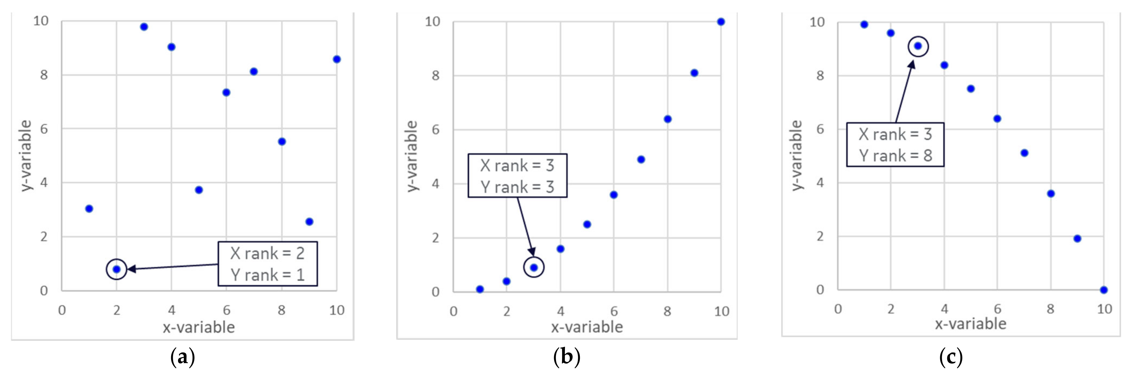
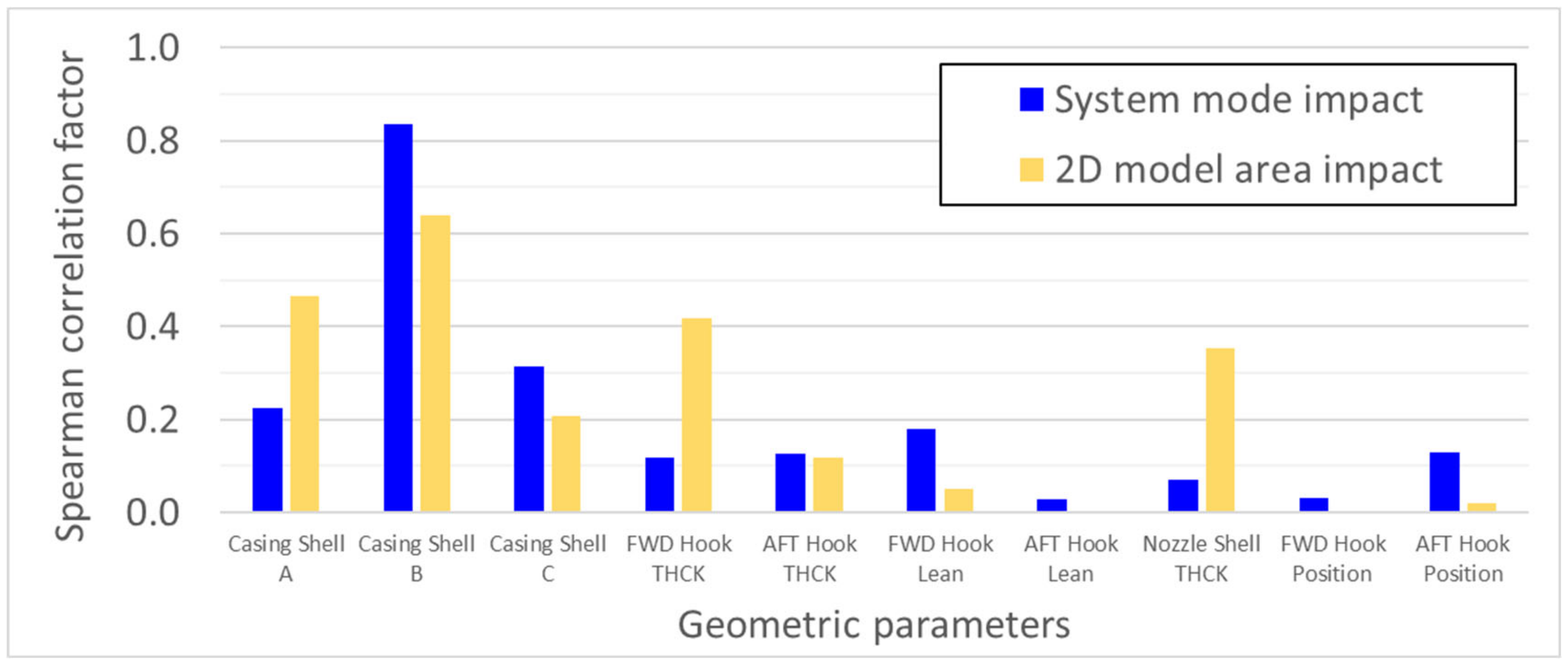
3.1. Sensitivity Analysis

To verify which geometrical parameters are impacting the natural frequency and model area, a sensitivity analysis using the Spearman correlation factor was performed. The correlation factor expresses to which extent two continuous data tend to change together. The factor described both the strength of the correlation and the direction and is in the range from −1 to +1. The correlation analysis presented in the article used the rank correlation coefficient applicable to analyze the data with non-linear dependance according to Equation (27).

$$\rho =1-\frac{6 {{\displaystyle \sum }}_{i=1}^n{\mathrm{d}}_i^2}{n^3-n}$$

(27)

where:

d_i—delta between x-variable rank and y-variable rank for each pair of data accordingly to the ascending order (see rank assignment example in Figure 14),

n—number of pair data (in example below is equal to 10).

Figure 14 shows the correlation coefficient (ρ) levels for three types of data representing no correlation (ρ = 0), strong positive (ρ = + 1) and negative (ρ = − 1) dependance between x and y tested variables.

Correlation coefficients against two y-variables are evaluated. The first is the natural frequency of the system mode and the second is the 2D model area impact. As x-variables, each of the geometrical features is described in the parameter’s definition section (Figure 12).

A review of the correlation coefficients presented in Figure 15 for the analyzed case reveals the high contribution of the casing shell B in the response for both system mode frequency (ρ = 0.83) and model area (ρ = 0.64). Nozzle pendulum mode shape induces the bending condition into casing where the forward and aft rails are moving off-phase (up and down). The thickness change is increasing overall system stiffness and directly affecting the natural frequency of the system. From the design change perspective, interesting characteristics are forward hook leaning and aft hook position since they can be neural for weight. No correlation on the response shows the rear hook leaning and the forward hook position.

3.2. Optimization Results

The genetic algorithm set of parameters are included in

Table 4. Genetic algorithm parameters.

Parameter Name	Value
Number of chromosomes in population	100
Convergence Stability Percentage	2
Mutation probability	0.01
Crossover probability	0.98
Maximum Number of Iterations	20
Maximum Number of Candidates	3 (best first 3 chromosomes)

. The optimization processes reported in Section 3.2.1, Section 3.2.2 and Section 3.2.3 are using the same set of algorithm parameters (Table 4).

An interpretation of the history charts is explained in Figure 16. It demonstrates the convergence progress from iteration to iteration. The first iteration is driven by random screening of the domain (initial population), while the second iteration shows the population created by the genetic algorithm through genetic operators. Between iterations the spread of the output parameter is reducing, reaching the convergence stability percentage criterion at the end.

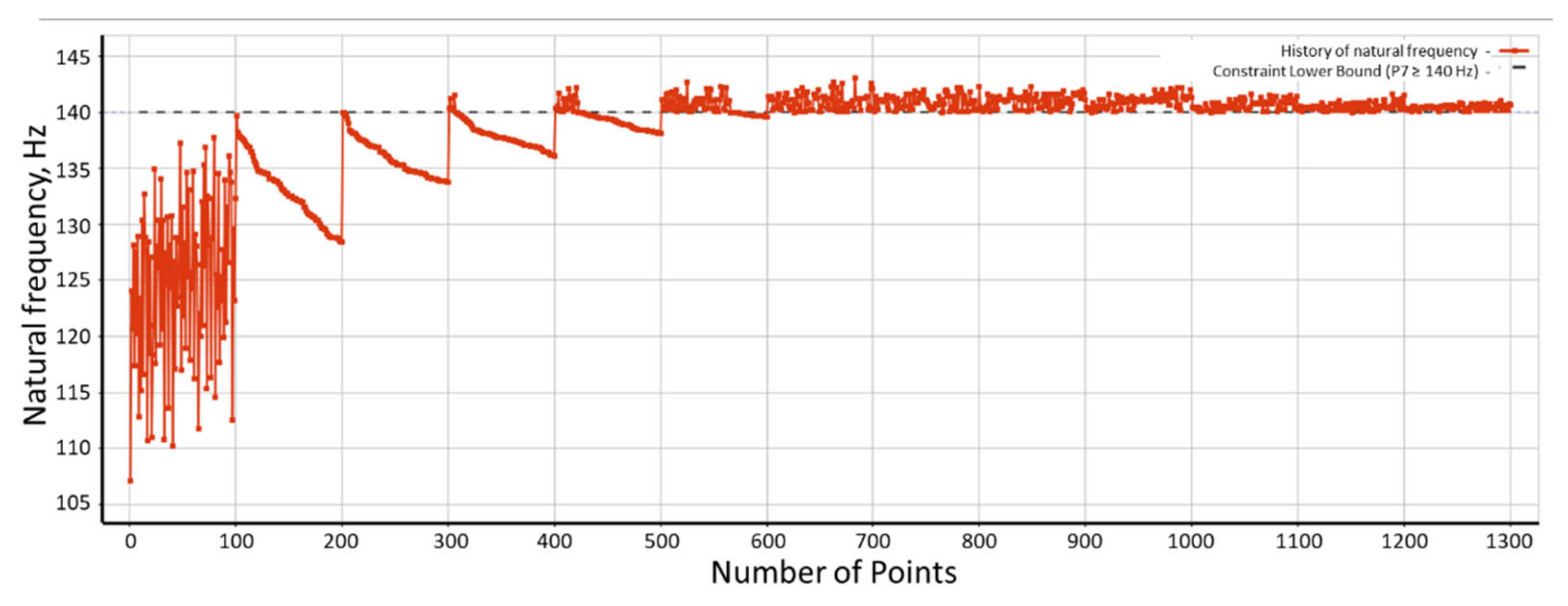
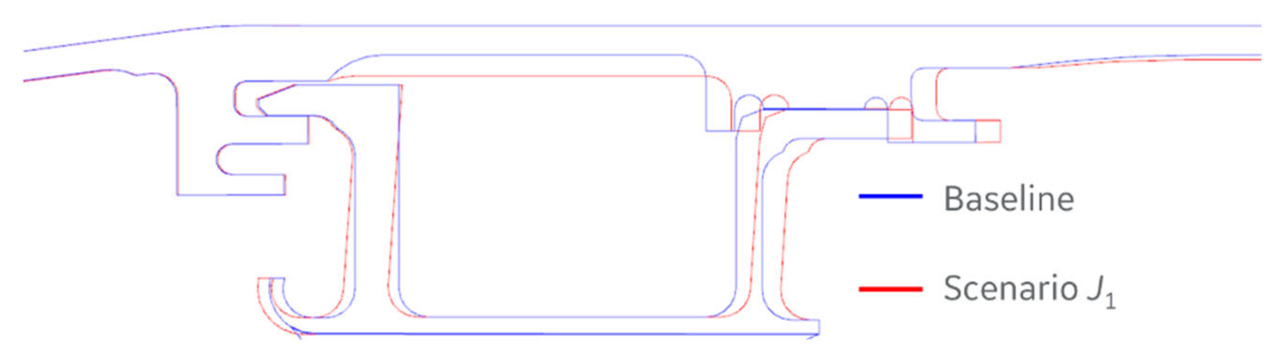
3.2.1. Optimization with Genetic Algorithm—Objective Function J₁

The first scenario of the optimization set a goal to minimize the model area and keep the first natural frequency above 140 Hz (level of the frequency derived from the domain screening) as reported in Equations (14) and (15). The history of the change in natural frequency of the first system mode is presented in t Figure 17.

Change history for the model area presented in Figure 18.

The algorithm converged after 1280 evaluations (13 iterations) to propose three candidates (the top three solutions) reported in detail in

Table 5. Optimization results—Objective function J₁.

Name	Baseline	Candidate 1	Candidate 2	Candidate 3
Shell_1_THCK (in)	0.100	0.105	0.106	0.105
Shell_2_THCK (in)	0.100	0.169	0.169	0.169
Shell_3_THCK (in)	0.100	0.114	0.115	0.114
FWD Hook THCK (in)	0.150	0.164	0.163	0.162
AFT Hook THCK (in)	0.090	0.101	0.102	0.107
FWD Hook Lean (degree)	90	85.007	84.742	87.618
AFT Hook Lean (degree)	90	80.949	82.309	82.062
Nozzle Shell THCK (in)	0.060	0.067	0.067	0.068
FWD Hook Pos (in)	0	0.013	0.013	0.014
AFT Hook Pos (in)	0	−0.046	−0.045	−0.042
1st System mode Frequency (Hz)	118.0	140.3	140.1	140.0
Geometry Surface Area (in2)	18.965	19.109	19.112	19.113

. The maximum number of iterations were not reached since the convergence stability percentage criterion was fulfilled earlier.

3.2.2. Optimization with Genetic Algorithm—Objective Function J_2A

As the second scenario included parameters associated with the nozzle only so hook thicknesses, position and leaning and nozzle outer band shell thickness. As a goal defined maximization of the natural frequency of the first system mode. The aim of the study is to verify if the same effect of frequency shift can be obtained excluding shell parameters on the casing. A history of the change in natural frequency of the first system mode is presented in Figure 19.

The algorithm converged after 1471 evaluations (15 iterations) to propose three candidates (the top three solutions) reported in detail in

Table 6. Optimization results—Objective function J_2A.

Name	Baseline	Candidate 1	Candidate 2	Candidate 3
Shell_1_THCK (in)	0.100
Shell_2_THCK (in)	0.100
Shell_3_THCK (in)	0.100
FWD Hook THCK (in)	0.150	0.198	0.200	0.198
AFT Hook THCK (in)	0.090	0.118	0.119	0.118
FWD Hook Lean (degree)	90	80.637	82.204	81.153
AFT Hook Lean (degree)	90	80.064	80.060	80.253
Nozzle Shell THCK (in)	0.060	0.076	0.086	0.087
FWD Hook Pos (in)	0	0.038	0.038	0.040
AFT Hook Pos (in)	0	−0.049	−0.047	−0.049
1st System mode Frequency (Hz)	118.0	128.6	128.6	128.6
Geometry Surface Area (in2)	18.965	19.049	19.061	19.062

. The maximum number of iterations were not reached since the convergence stability percentage criterion was fulfilled before.

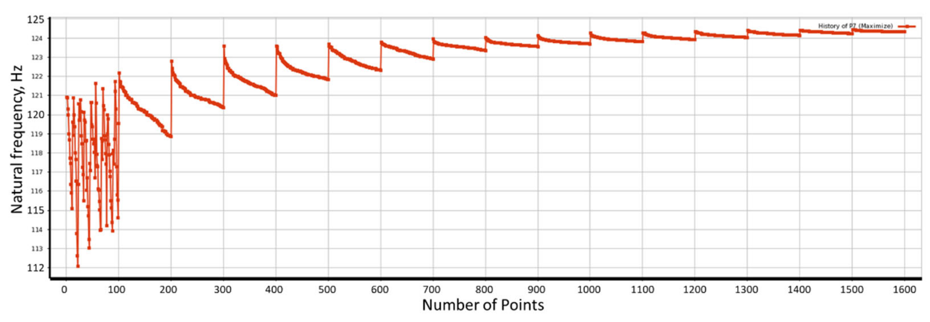
3.2.3. Optimization with Genetic Algorithm—Objective Function J_2B

The third scenario excludes any thickness characteristics that affect nozzle and casing weight. Accounted in process only forward and rear hook positions and leaning. As a goal set to maximize the natural frequency of the first system model. The history of the change in natural frequency of the first system mode is presented in Figure 20.

The algorithm converged after 1569 evaluations (16 iterations) to propose three candidates (the top three solutions) reported in detail in

Table 7. Optimization results—Objective function J_2B.

Name	Baseline	Candidate 1	Candidate 2	Candidate 3
Shell_1_THCK (in)	0.100
Shell_2_THCK (in)	0.100
Shell_3_THCK (in)	0.100
FWD Hook THCK (in)	0.150
AFT Hook THCK (in)	0.090
FWD Hook Lean (degree)	90	80.577	80.013	80.122
AFT Hook Lean (degree)	90	80.329	80.343	80.446
Nozzle Shell THCK (in)	0.060
FWD Hook Pos (in)	0	0.037	0.038	0.036
AFT Hook Pos (in)	0	−0.050	−0.050	−0.050
1st System mode Frequency (Hz)	118.0	124.4	124.4	124.4
Geometry Surface Area (in2)	18.965	18.978	18.978	18.979

. Maximum number of iterations were not reached since fulfilled convergence stability percentage criterion.

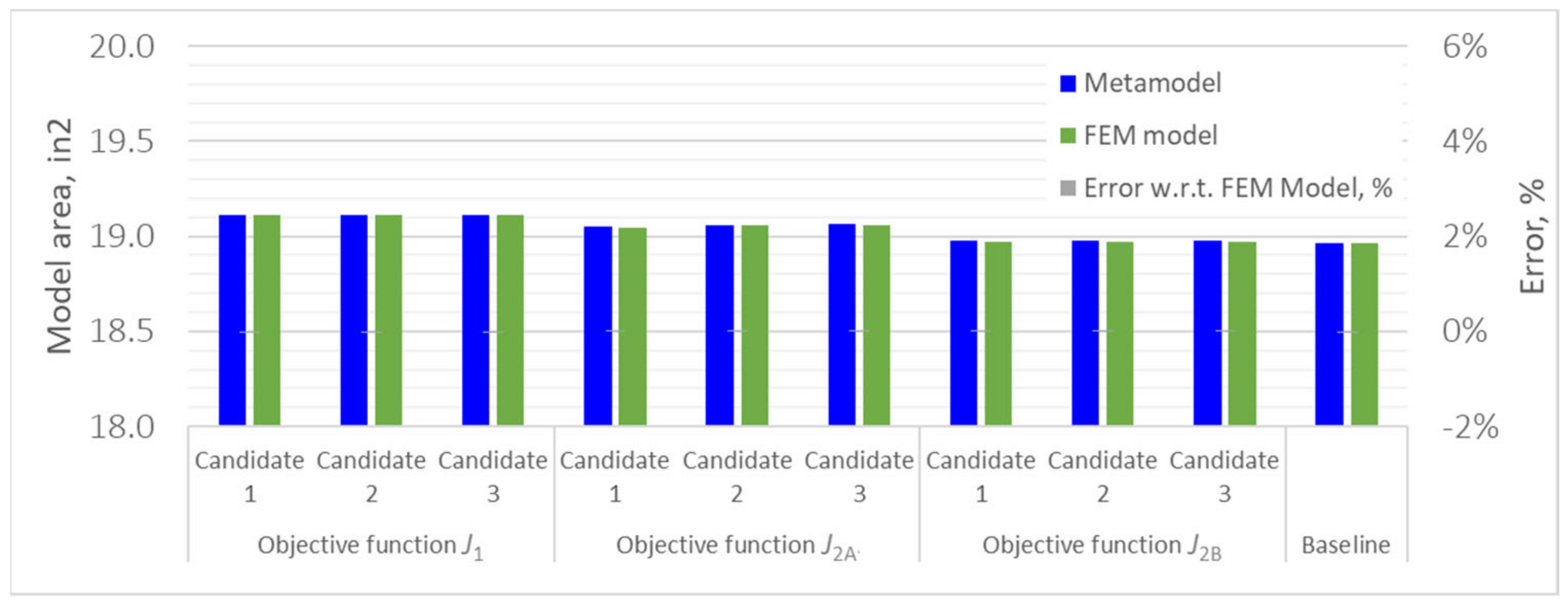
3.3. Optimization Summary

Optimization results obtained from the metamodel were verified using the FEM method and are compared in Figure 21.

The maximum error was found for the metamodel with 10 parameters set and is equal to 2%. The results have been summarized Figure 22 and

Table 8. Results of the optimization process.

	Baseline	Objective Function
		J1	J2A	J2B
Frequency, Hz	118.03	143.2	128.2	123.6
Model area, in2	18.965	19.111	19.047	18.972
Frequency shift, %		21%	9%	5%
Effectiveness Area/Freq shift (Area cost per 1 Hz)		0.006	0.008	0.001

, showing candidates obtained from optimization processes together with a baseline for reference using validated FEM data.

The highest frequency shift is obtained for the scenario with objective function J₁ (10 geometrical variables set) and is equal to 21%. At the same time, this solution shows the highest impact on model area so in consequence it also affects the component’s weight. The scenario reported as objective function J_2A (geometrical parameters associated with nozzle only) is not able to reach the same frequency shift as for the optimization process with all parameters included. Moreover, effectiveness was calculated (Equation (28)), so the cost in terms of area per one Herz is similar between J₁ and J_2A.

$$Effectivness=\frac{A_{CANDIDATE}-A_{BASELINE}}{f_{CANDIDATE}-f_{BASELINE}}$$

(28)

The only valuable solution from a weight perspective is J_2B (parameters related only to forward and rear hook position and leaning). The obtained frequency shift is 5% and is limited by the geometrical parameter’s lower and upper bounds.

A geometry comparison between baseline configuration (blue lines) and proposed design (red lines) has been reported in Figure 23 for scenario J₁ and Figure 24 for scenario J_2B. The main difference is related to the casing shell thickness between the rails and the hook leaning.

The number of iterations varies from 13 for scenario J₁ to 16 for scenario J_2B. The main reason why the iteration number increases is related to the available parameters for the optimization task and how the convergence stability percentage criterion is defined. The denominator in Equations (25) and (26) will be greater for scenario J₁ compared to scenario J_2B, leading to a tighter convergence criterion for scenarios with parameters associated with the hook position and leaning. To keep the same absolute criterion on output percentage should be adjusted. Since the entire process is based on the meta model, the difference in the number of evaluations and iterations has no adverse impact on analysis time.

4. Discussion

For the defined parameter domain, the maximum frequency shift is equal to 21% and is obtained by setting mainly the casing shell, nozzle hooks and outer band shell thicknesses in upper spec limit. The described modification leads to an increase of system stiffness that results in frequency increase accordingly to the fundamental equation presented for the harmonic oscillator. The study clearly indicates the casing shell thickness in between nozzle hooks with the highest correlation coefficient for the first system mode response among all other design variables. At the same time, this characteristic has the highest impact on the model area and therefore on component weight. The promising solution from a weight impact perspective is the one related to hook position and leaning that demonstrates a frequency shift with no adverse impact on component weight. The limited frequency shift for this solution is driven by the defined parameter range.

The studied solution does not affect the position or shape of the aerodynamic profile that is also a constraint in the optimization process. The flowpath side is fixed in order to not affect the aerodynamic characteristics.

The optimization process is working on the meta-model, therefore it is very robust even if number of evaluation cases is reaching more than 1300 design points. The presented correlation coefficient chart reported in Figure 15 provides guidance for a design engineer in terms of the impact on the first system mode and the model area.

The noticed difference of a maximum 2% on the natural frequency between applied to the surrogate model and the FEM results. For optimization purposes, the reported shift is considered acceptable and proves the good quality of the meta model.

For future optimization processes, it is recommended that the parameter range associated with the hook position and leaning be extended so that it has no adverse impact on system weight.

References

1. Geradin, M.; Rixen, D.J. Mechanical Vibrations; Wiley: Hoboken, NJ, USA, 2015. [Google Scholar]
2. Case, J.; Chilver, A.H. Strength of Materials and Structures; Edward Arnold: Baltimore, MD, USA, 1986. [Google Scholar]
3. Zienkiewicz, O.C. The Finite Element Method in Structural and Continuum Mechanics; McGraw-Hill: New York, NY, USA, 1971. [Google Scholar]
4. Flemming, S. Performance optimization of gas turbine engines using STUDGA. In Proceedings of the 14th Triennial World Congress, Beijing, China, 5–9 July 1999. [Google Scholar]
5. Davari, A.R.; Hasheminejad, M.; Boorboor, A. Shape Optimization of Wind Turbine Airfoils by Genetic Algorithm. IACSIT Int. J. Eng. Technol. 2013, 5, 206. [Google Scholar] [CrossRef]
6. Cao, J.; Luo, Y.; Umar, B.M.; Wang, W.; Wang, Z. Influence of structural parameters on the modal characteristics of a Francis runner. Eng. Fail. Anal. 2022, 131, 105853. [Google Scholar] [CrossRef]
7. Soares, C. Gas Turbines: A Handbook of Air, Land and Sea Applications; Chapter 1: Gas Turbines: An Introduction and Applications; Elsevier: Amsterdam, The Netherlands, 2011. [Google Scholar]
8. Soares, C. Gas Turbines: A Handbook of Air, Land and Sea Applications; Chapter 10: Performance, Performance Testing, and Performance Optimization; Elsevier: Amsterdam, The Netherlands, 2011. [Google Scholar]
9. Rakowski, G.; Kacprzyk, Z. Metoda Elementów Skończonych w Mechanice Konstrukcji; Oficyna Wydawnicza Politechniki Warszawskiej: Warsaw, Poland, 1993. [Google Scholar]
10. Holland, J.H. Outline for biological theory of adaptive systems. J. ACM 1962, 3, 297–314. [Google Scholar] [CrossRef]
11. Arbor, A.; Holland, J.H. Adaptation in Natural and Artificial Systems; The University of Michigan Press: Ann Arbor, MI, USA, 1975. [Google Scholar]
12. Holland, J.H.; Reitman, J.S. Cognitive Systems Based on Adaptive Algorithms, Pattern-Directed Inference Systems; Academic Press: New York, NY, USA, 1978. [Google Scholar]
13. Darwin, C.; Smith, S.; Rachootin, S.P. Charles Darwin’s Natural Selection; Cambridge University Press: Cambridge, UK, 1987. [Google Scholar]
14. Goldberg, D.E. Algorytmy Genetyczne i ich Zastosowania; Wydawnictwo Naukowo-Techniczne: Warszawa, Poland, 1995. [Google Scholar]
15. Viana, F.A.C.; Haftka, R.T.; Steffen, V. Multiple Surrogates: How Cross-Validation Errors Can Help Us to Obtain the Best Predictor. Struct. Multidiscip. Optim. 2009, 39, 439–457. [Google Scholar] [CrossRef]
16. Salem, B.; Roustant, O.; Gamboa, F.; Tomaso, L. Universal prediction distribution for surrogate models. SIAM/ASA J. Uncertain. Quantif. 2017, 5, 1086–1109. [Google Scholar] [CrossRef]
17. Acar, E. Various Approaches for Constructing an Ensemble of Metamodels Using Local Measures. Struct. Multidiscip. Optim. 2010, 42, 879–896. [Google Scholar] [CrossRef]
18. Available online: https://www.ansys.com/ (accessed on 9 May 2022).
19. Gill, P.E.; Murray, W.; Saunders, M.A.; Wright, M.H. Sequential Quadratic Programming Methods for Nonlinear Programming. In Computer Aided Analysis and Optimization of Mechanical System Dynamics; NATO ASI Series (Series F: Computer and Systems Sciences); Haug, E.J., Ed.; Springer: Berlin/Heidelberg, Germany, 1984; Volume 9. [Google Scholar]
20. Exler, O.; Schittkowski, K.; Lehmann, T. A comparative study of numerical algorithms for nonlinear and nonconvex mixed-integer optimization. Math. Program. Comput. 2012, 1, 383–412. [Google Scholar] [CrossRef]
21. Exler, O.; Schittkowski, K. A trust region SQP algorithm for mixed-integer nonlinear programming. Optim. Lett 2007, 1, 269–280. [Google Scholar] [CrossRef]
22. Exler, O.; Lehmann, T.; Schittkowski, K. MISQP: A Fortran Subroutine of a Trust Region SQP Algorithm for Mixed-Integer Nonlinear Programming—User’s Guide Report; Department of Computer Science, University of Bayreuth: Bayreuth, Germany, 2012. [Google Scholar]
23. Yang, X.-S. Nature-Inspired Optimization Algorithms; Elsevier: Amsterdam, The Netherlands, 2014. [Google Scholar]
Figure 1. Diagram of two spool turbofan engine [7].
Applsci 12 09724 g001
Figure 2. P-v and T-s diagrams of an ideal Brayton cycle.
Applsci 12 09724 g002
Figure 3. Notional Goodman diagram.
Applsci 12 09724 g003
Figure 4. Harmonic oscillator.
Applsci 12 09724 g004
Figure 5. Notional Campbell diagram.
Applsci 12 09724 g005
Figure 6. Notional Campbell diagram with optimal location of the natural frequency mode.
Applsci 12 09724 g006
Figure 7. First system mode of the nozzle-casing system.
Applsci 12 09724 g007
Figure 8. Genetic algorithm flowchart.
Applsci 12 09724 g008
Figure 9. Aggregated metamodel example for 1D function.
Applsci 12 09724 g009
Figure 10. Approach for two-dimensional analysis.
Applsci 12 09724 g010
Figure 11. FEM model: boundary conditions and contact area between nozzle and casing.
Applsci 12 09724 g011
Figure 12. Geometrical parameters dedicated for optimization.
Applsci 12 09724 g012
Figure 13. Optimization framework with metamodel.
Applsci 12 09724 g013
Figure 14. Correlation coefficient interpretation: (a) No correlation ρ = 0; (b) Strong positive correlation ρ = + 1; (c) Strong negative correlation ρ = − 1.
Applsci 12 09724 g014
Figure 15. Spearman correlation factor for analyzed responses.
Applsci 12 09724 g015
Figure 16. Interpretation of the convergence diagram (history chart).
Applsci 12 09724 g016
Figure 17. Convergence history for first mode natural frequency.
Applsci 12 09724 g017
Figure 18. Convergence history for model area.
Applsci 12 09724 g018
Figure 19. Convergence history for first mode natural frequency.
Applsci 12 09724 g019
Figure 20. Convergence history for the first mode’s natural frequency.
Applsci 12 09724 g020
Figure 21. Metamodel validation with FEM model results.
Applsci 12 09724 g021aApplsci 12 09724 g021b
Figure 22. Optimization summary results with baseline for reference.
Applsci 12 09724 g022
Figure 23. Geometry comparison between baseline and proposed configuration (scenario J1).
Applsci 12 09724 g023
Figure 24. Geometry comparison between baseline and proposed configuration (scenario J2B).
Applsci 12 09724 g024