Performance Optimization Design of Diagonal Flow Fan Based on Ensemble of Surrogates Model

Abstract

Due to the advantages of a high total pressure coefficient, large flow coefficient, and high efficiency, the diagonal flow fan is widely used in people’s livelihood and industrial fields. However, the design of the diagonal flow fan is mostly empirical, multi-solution, and comprehensive. The traditional optimization design process often consumes huge computing resources. In this paper, the diagonal flow fan blade is parameterized, the design variables are determined, and the accuracy of the parameterization method is verified. The maximum fitting error is controlled at approximately 0.1%. Based on the parametric design of blades, this paper organically integrates the traditional Kriging model and RBF model, and introduces the Ensemble of surrogates model (ES) to verify that the ES model has higher prediction accuracy in the prediction of fan flow and total pressure efficiency than the traditional prediction model. Subsequently, the Pareto optimal solution set of the approximate model within the global design scope is searched by NSGA-II. The numerical simulation and experimental verification show that the actual flow of the fan increases by 10% and the efficiency of the full pressure increases by 3.2% under the design condition of the optimized blade. The optimized model can significantly improve its air performance.

1. Introduction

The impeller hub of the diagonal flow fan is conical. It is a kind of fan whose gas enters from the axial direction, exports along the inclined direction of the impeller, and discharges from the axial direction after turning through the air duct [1,2]. It is widely used in chemical industry, metallurgy, energy, construction, agriculture, and other fields because of its high total pressure coefficient, large flow coefficient, high efficiency, and wide working range [3]. With the increasing global energy consumption, the international community is increasingly calling for energy conservation and environmental protection, as well as the huge energy consumption and serious noise pollution of the fan system. It is urgent for the fan industry to have the ability to quickly design and manufacture high-efficiency and low-noise diagonal flow fans. However, the large demand for diagonal flow fans does not match the development of its design methods. The existing design theory of diagonal flow fan or diagonal flow impeller mainly focuses on the application fields of aeroengine and compressor with high speed, a high pressure ratio, and compressible gas. There are a few performance optimization methods for small diagonal flow fans under low speed and incompressible gas conditions [4,5].

The diagonal flow impeller, with its unique performance advantages, has drawn the attentionof many scholars at home and abroad. For example, Furukawa et al. [6] carried out numerical simulation and experimental research on the leakage vortex and diffusion development process at the tip clearance of the diagonal flow fan. The results show that the tip leakage vortex rupture occurs at the tail of the fan blade passage, and the leakage vortex rupture directly leads to the vortex core disappearing, an increase in the leakage vortex diffusion degree in the flow passage, and the formation of the low-pressure area. Jin et al. [7] studied the three-dimensional flow stability expansion mechanism of a low-pressure axial fan, and verified the influence of curved blades on boundary layer migration through experiments. FUNAKOSHI et al. [8] revealed the unsteady flow characteristics of the flow field in the diagonal flow pump. Studies have shown that the tip leakage flow was entrained with the mainstream in the blade channel, resulting in the tip leakage vortex. The blade inlet easily formed a separation vortex due to flow separation. Based on a BP neural network and a genetic algorithm, YANG [9] et al. optimized the blade of a low-pressure axial flow fan. The results show that the forward-curved blade can redistribute the airflow along the blade span and reduce the tip load, thus improving the operating performance and total pressure ratio of the fan while expanding the stable operation range of the fan.

At present, the design of diagonal flow fan products presents the characteristics of experience, multiple solutions, and comprehensiveness. The solution process is the cross-integration of machinery, computer science, mathematics, and other disciplines. The optimization design process often requires huge computational resources. This problem can be solved by establishing a surrogate model based on limited experiments instead of complex simulation calculations. The traditional single surrogate model does not always obtain the complex nonlinear relationship between variables and objectives, while the combination of multiple surrogate models, without increasing the computational cost of optimization, can integrate the advantages of various surrogate models to improve the possibility of obtaining the optimal solution [10,11].

Based on the equivalent simplified impeller model established by the parametric design of the diagonal flow fan blade, this paper establishes the Ensemble of surrogates model based on the multi-domain mapping of the fan system, realizes the establishment of an efficient engineering model for prediction analysis and performance verification, and coordinates the contradiction between model accuracy and calculation efficiency. Finally, the optimization design of fan performance is realized by repeated iterations of a genetic algorithm.

2. Research Object and Method

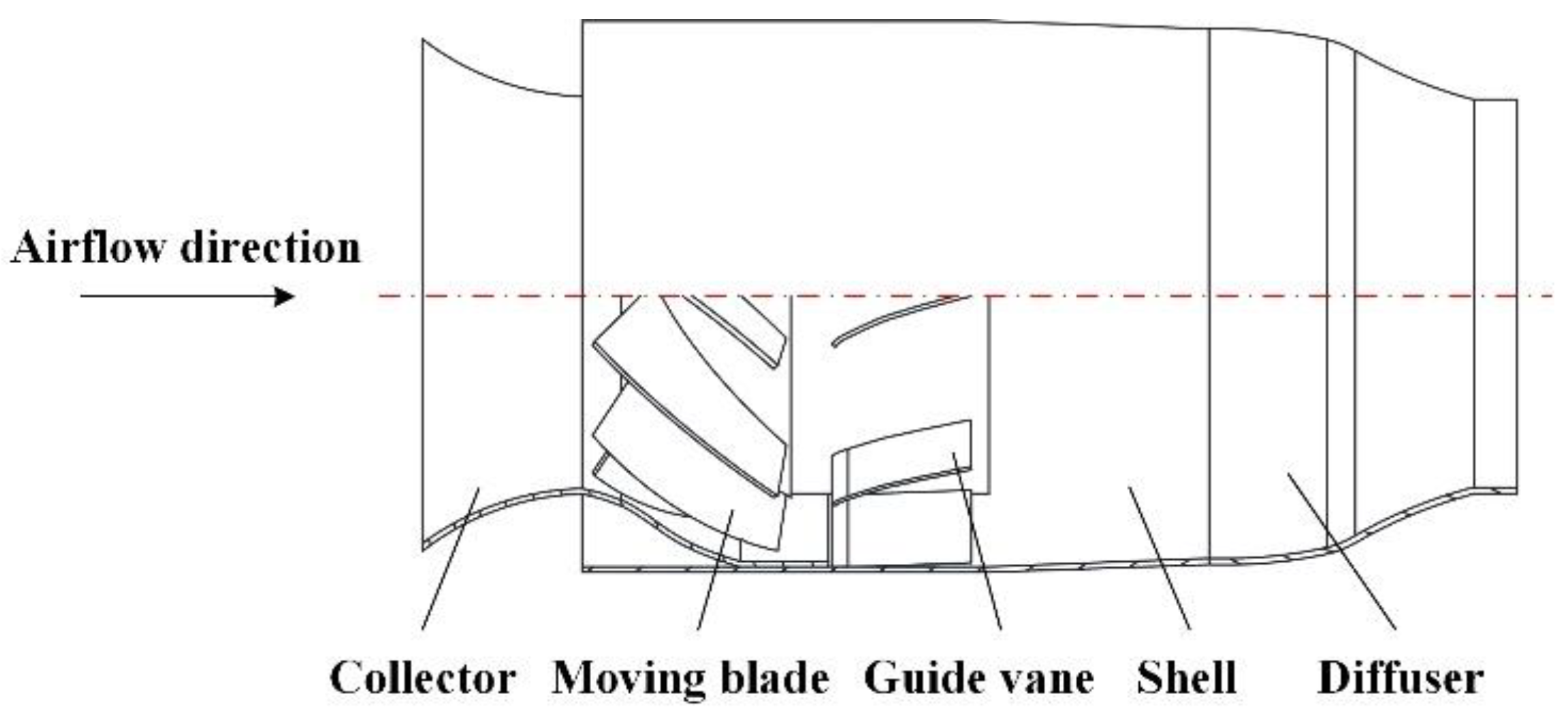
2.1. Research Object

A small diagonal flow fan was studied in this research. The main structure is shown in Figure 1. Its flow components are mainly composed of a collector, moving blade, guide vane, and diffuser, in which the impeller is the only working element. The structural parameters were as follows: Impeller inlet outer diameter D_in = 175 mm, impeller outlet outer diameter D_out = 235 mm, blade number Z = 10, guide vane blade number 9, rotation speed n = 2000 r/min, and flow rate Q = 19.4 m³/min at 25 °C.

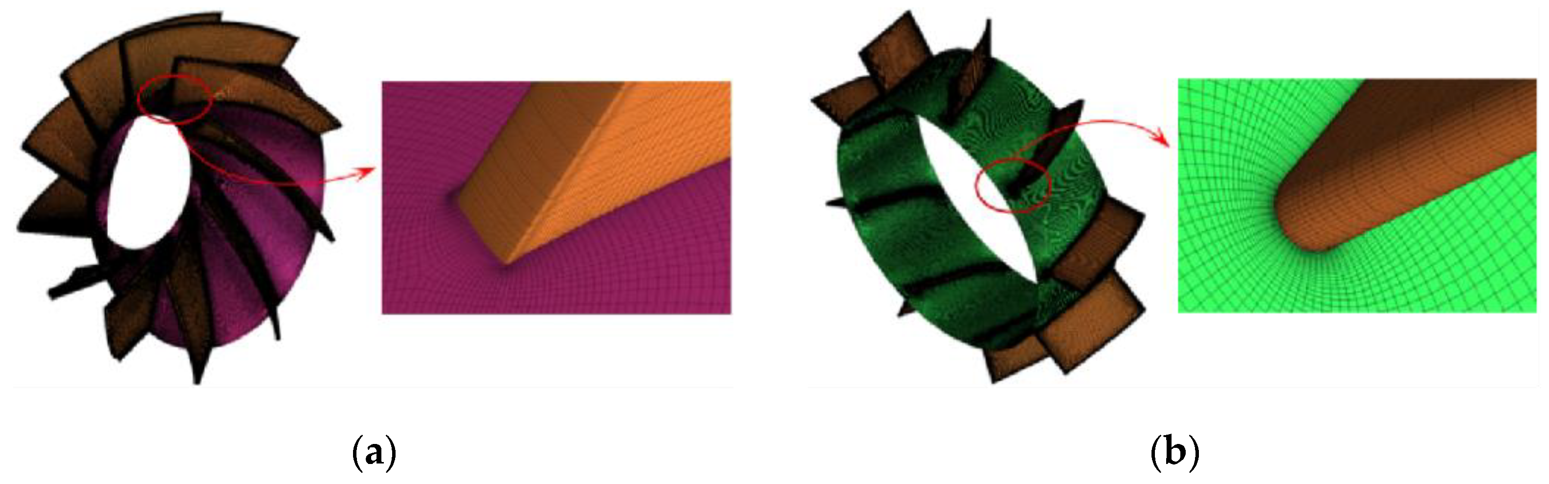
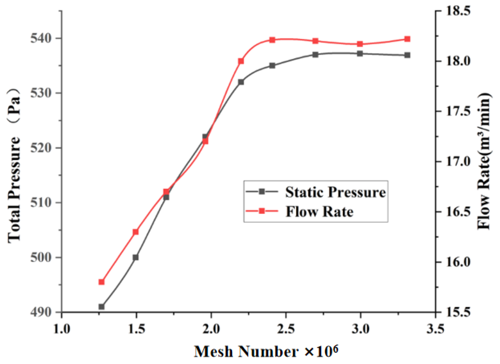
2.2. Computational Model and Mesh Blocking

We simplified the physical model and selected the fan flow components. At the same time, in order to improve the accuracy of fan performance prediction, the inlet and outlet areas were extended, and the extension length was 5 times the outlet diameter. According to the actual position of the rotating parts and the static parts of the fan, the whole diagonal flow fan basin was divided into five parts, which are the inlet basin, moving blade basin, guide vane basin, diffuser basin, and outlet basin. Figure 2 is the simplified fan basin diagram.

Grid blocking of five different basins was carried out. Because the simulation results are greatly affected by the grid, in order to improve the calculation accuracy, TurboGrid was used to generate the structural grid for the rotor blade basin and the guide vane basin of the core components of the fan, and the rest of the flow components were unstructured. Figure 3a shows the grid of the impeller region, and Figure 3b shows the grid diagram of the guide vane area. When meshing, the first node must be located in the viscous bottom layer. The dimensionless distance between the first grid and the wall is generally expressed by y+, and it is generally believed that the y+ value here is less than 5 [12]. The empirical formula of y+ is:

$$Y_{wall}=6{\left(\frac{V_{ref}}{v}\right)}^{-\frac{7}{8}}{\left(\frac{L_{ref}}{2}\right)}^{\frac{1}{8}}{y}^{+}$$

(1)

where V_ref is the reference speed, m/s; L_ref is the reference length, m; v is the kinematic viscosity of fluid, m²/s; and y⁺ is a dimensionless parameter. The grid height of the first layer of the boundary layer should be less than 0.6 mm calculated by an empirical formula.

After the grid quality meets the requirements, it is also necessary to verify the independence of the number of computational grids. Too few grids can easily make the calculation results unstable, but when the number of grids reaches a certain threshold, the calculation accuracy is difficult to improve. As shown in Figure 4, when the total number of fan nodes reaches approximately 2.5 × 10⁶, the calculation results of the fan flow and total pressure remain basically stable. Therefore, considering the relationship between the prediction accuracy and computation time, the selected computational number of nodes is 2,709,026.

3. Calculation Method and Verification

3.1. Method of Calculation

The turbulent development in the near-wall region of the small low-speed diagonal flow fan studied in this paper is not sufficient, and the influence of turbulent pulsation on the fluid motion may be less than that of molecular viscosity. Considering the internal curved streamline of the diagonal flow fan, the turbulence is anisotropic, and the viscosity coefficient µ_t should be an anisotropic scalar value. Therefore, the realizable k-ε model is selected to modify this point. The mathematical expression of the model for the flow problem of the diagonal flow fan is:

$$\frac{\partial \left(\rho k\right)}{\partial t}+\frac{\partial \left(\rho k{u}_i\right)}{\partial x_i}=\frac{\partial }{\partial x_i}\left[\left(\mu +\frac{{\mu }_t}{{\sigma }_k}\right)\frac{\partial k}{\partial x_i}\right]+G_k-\rho \epsilon$$

(2)

$$\frac{\partial \left(\rho \epsilon \right)}{\partial t}+\frac{\partial \left(\rho \epsilon u_i\right)}{\partial x_i}=\frac{\partial }{\partial x_i}\left[\left(\mu +\frac{{\mu }_t}{{\sigma }_k}\right)\frac{\partial \epsilon }{\partial x_i}\right]+\rho C_{1}E\epsilon -\rho C_2\frac{{\epsilon }^2}{k+\sqrt{v\epsilon }}$$

(3)

In the formula:

$$\begin{array}{l}{\sigma }_k=1.0\hspace{1em}{\sigma }_s=1.2\hspace{1em}{C}_2=1.9\\ C_1=\max \left(0.43,\frac{\eta }{\eta +5}\right)\\ \eta ={\left(2E_{ij}·E_{ij}\right)}^{0.5}\frac{k}{\epsilon }\\ E_{ij}=\frac{1}{2}\left(\frac{\partial u_i}{\partial x_j}+\frac{\partial u_j}{\partial x_i}\right)\end{array}$$

(4)

The flow medium selected was 25 °C air, and the rotating domain is the impeller basin. The multiple reference frame model (MRF) is used for calculation. The rotating speed of the impeller is 2000 rpm, and the inlet and outlet boundary conditions are pressure-inlet and pressure-outlet, respectively. The solution is based on the implicit solution of pressure. We solved the three-dimensional Reynolds average N-S equation using the realizable k-ε model. The SIMPLE algorithm was selected to couple the velocity and pressure. A second-order upwind scheme was adopted for all spatial discrete schemes. When the root mean square (RMS) of the residuals of each control equation was less than 1 × 10⁻⁵, the calculation was considered to be convergent.

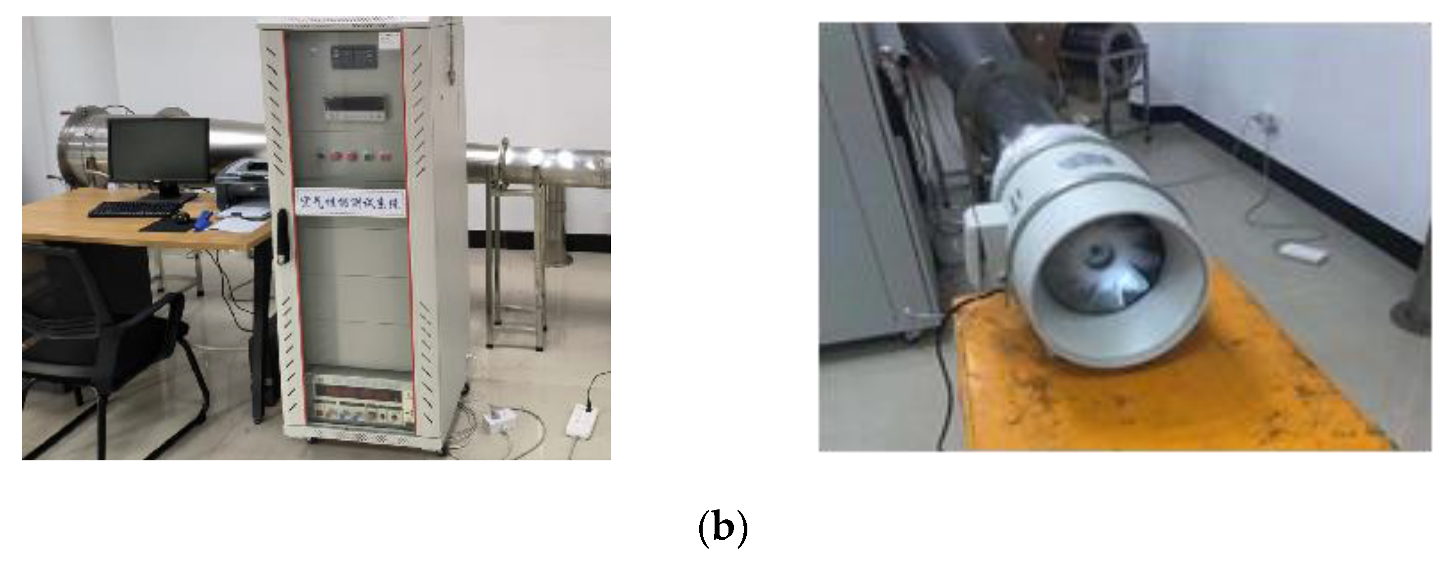
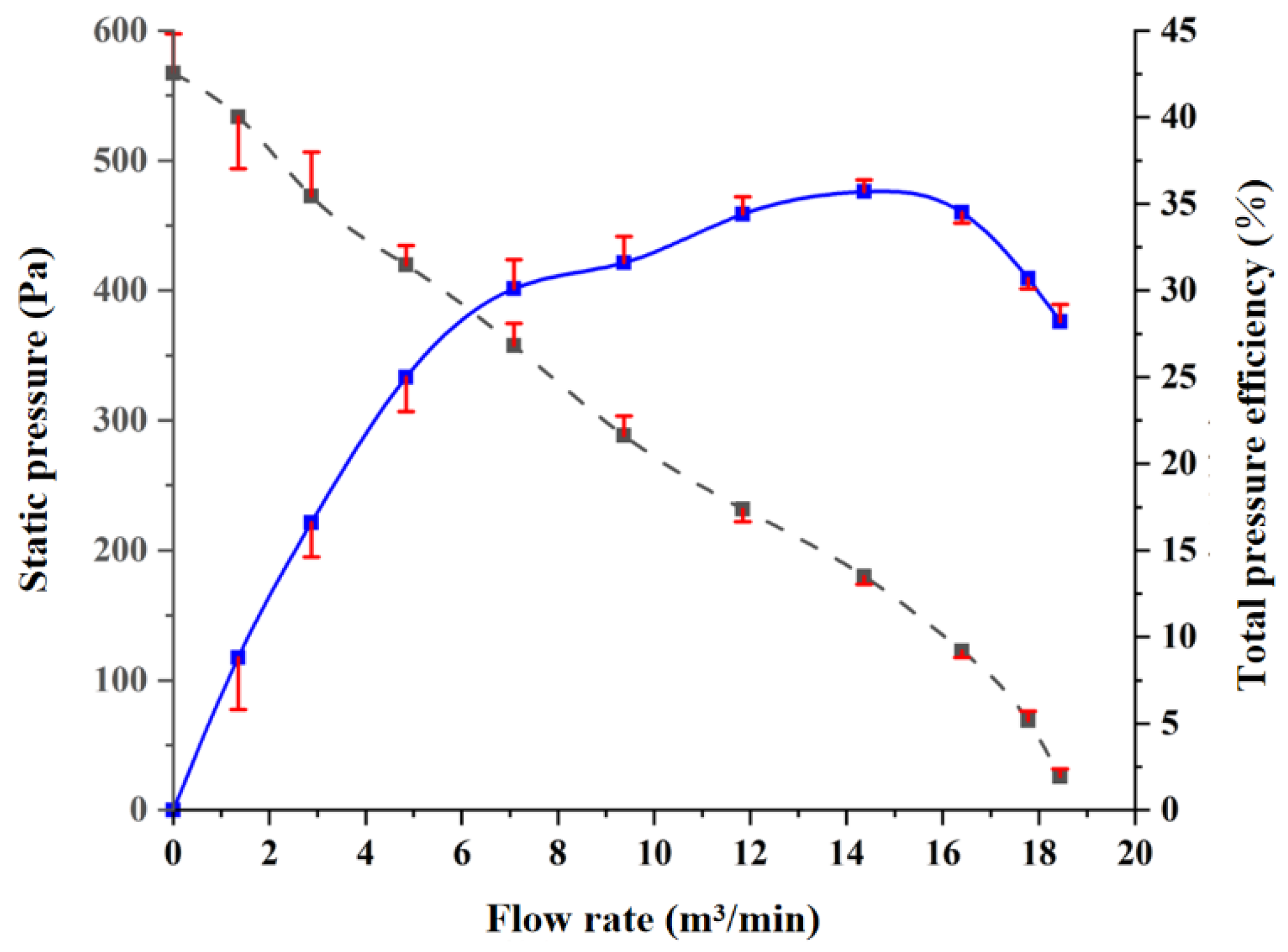
3.2. Fan External Characteristic Test

According to the regulations and requirements of ‘Fans—Performance testing using standardized airways (ISO 5801:2017)’ [13], the air performance of the small diagonal flow fan in this paper was tested with the air flow test bench. Figure 5 shows the air test rig device diagram and field test picture. To reduce the test error and ensure the accuracy of test results, the mixed-flow fan was operated at 220 V standard voltage for 30 min and tested when the performance was stable. Parameter sensors such as pressure, temperature, and humidity weere arranged inside the test pipe, which were imported into the computer and converted into relevant air parameters after formula calculation. In the test process, it is necessary to control the outlet diameter of the air duct by replacing the orifice plate to realize the air performance test of the fan under different flow conditions.

In order to compare the error between the predicted value of the calculation model and the true value of the test, the calculation results are compared with the experimental values to obtain the flow-static pressure-total pressure efficiency performance curve shown in Figure 6.

It can be seen from the external characteristic curve of Figure 6 that the predicted value is close to the experimental value, and their changing trends are basically consistent. Under the condition of a small flow rate, due to the influence of turbulence and boundary layer separation, there is still a certain deviation between the simulated and experimental values. However, this paper studies the operating performance of the diagonal flow fan under standard operating conditions. Under the design conditions, the error between the experimental value and the calculated value of the diagonal flow fan is basically controlled to within 3%, which is significantly less than the engineering calculation error requirements [14]. Therefore, the numerical simulation method is considered to be more reliable and can be used for subsequent optimization calculations.

4. Ensemble of Surrogate Model and Multi-Objective Optimization

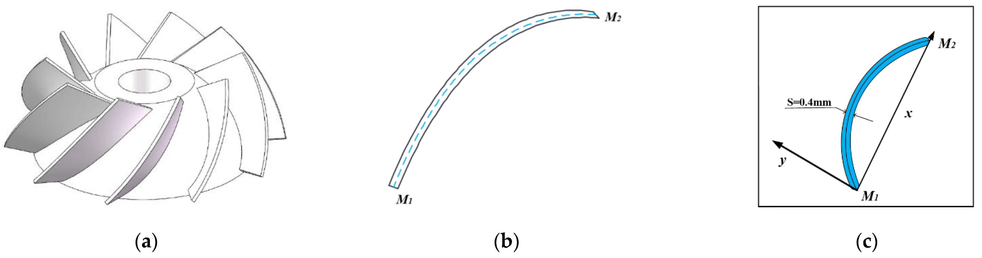
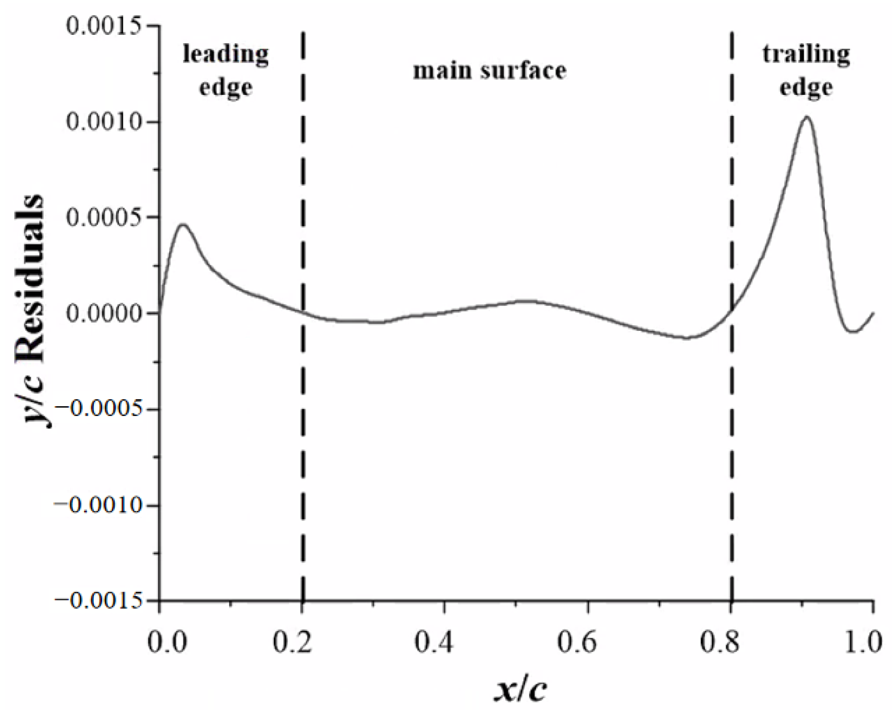
4.1. Parameterized Design of Blade

Kulfan B [15,16] first proposed the CST parameterization method in 2006. This method determines the basic shape of airfoil based on the class function and corrects its shape parameters using the shape function. The research shows that the CST parameterization method has the advantages of adjustability, fewer design variables, and a wide design range. The technology is combined here with the design of the middle arc of the blade of the small diagonal flow fan, as shown in Figure 7.

As shown in Figure 7a, the three-dimensional diagram of the diagonal flow fan impeller in this paper is shown. In Figure 7b, the xOy coordinate system is constructed with M₁ in a single blade as the starting point and M₂ as the end point. The parameterized blade has fixed endpoints M₁ and M₂, so the blade chord length c remains unchanged, as shown in Figure 7c.

Usually, the airfoil curve can be expressed by the CST parameterization method as:

$$\frac{y}{c}=C\left(\frac{x}{c}\right)S\left(\frac{x}{c}\right)+\frac{x}{c}\frac{\Delta z_{te}}{c},0\le \frac{x}{c}\le 1$$

(5)

where C(x/c) and S(x/c) are the class function and shape function, respectively; c is the chord length of the airfoil; and Δz_te is the trailing edge thickness of the airfoil, where Δz_t is 0.

$$C\left(\frac{x}{c}\right)={\left(\frac{x}{c}\right)}^{N_1}{\left(1-\frac{x}{c}\right)}^{N_2}$$

(6)

In Formula (6), the airfoil type is determined by N₁ and N₂. For the parametric design of airfoil, let N₁ = 0.75 to ensure the circular leading edge; let N₂ = 0.75, guaranteeing the circular airfoil trailing edge.

The shape function S(x/c) controls the curve modeling between the two points of the leading edge and the trailing edge of the airfoil, generally expressed in the Bernstein polynomial form by introducing a weighting factor. The weighted sum of the n-order Bernstein polynomials is:

$$\begin{array}{l}S\left(\frac{x}{c}\right)={\displaystyle \sum _{i=0}^n\left[b_i\cdot K_{i,n}\cdot {\left(\frac{x}{c}\right)}^i\cdot {\left(1-\frac{x}{c}\right)}^{n-i}\right]}\\ K_{i,n}=\frac{n!}{i!\left(n-i\right)!}\end{array}$$

(7)

Among them, K_i,n is the binomial coefficient, b_i is the weight factor, and n is the polynomial order. Usually, the higher the order is, the higher the accuracy of the airfoil is. Considering the fitting accuracy and engineering application, n = 3 is selected, that is, the third-order polynomial only needs four variables.

In summary, the arc of the small diagonal flow fan blade in this paper can be expressed as:

$$\begin{array}{l}{a}_i\left(x\right)=C\left(x\right)\cdot S\left(x\right)\\ a_i\left(x\right)=x^{0.75}\cdot {\left(1-x\right)}^{0.75}\cdot {\displaystyle \sum _{i=0}^n{v}_i{x}^i{\left(1-x\right)}^{n-i}}\end{array}$$

(8)

where v₀, v₁, v₂, and v₃ are the four design variables in this paper.

In order to explore the accuracy of CST parametric design of the blade camber line, the y/c residual is introduced to characterize the fitting error:

$$y/c Residuals=\frac{y/c-y/c^{\prime }}{y-c}$$

(9)

As shown in Figure 8, the arc error analysis of the blade is fitted using the CST parametric design method. It can be seen from the diagram that the error is higher at the leading edge and the trailing edge, and the maximum error point appears near the trailing edge, reaching 0.00105. Therefore, when the maximum fitting error is only 0.1%, this paper suggests that the parametric design method meets the accuracy requirements.

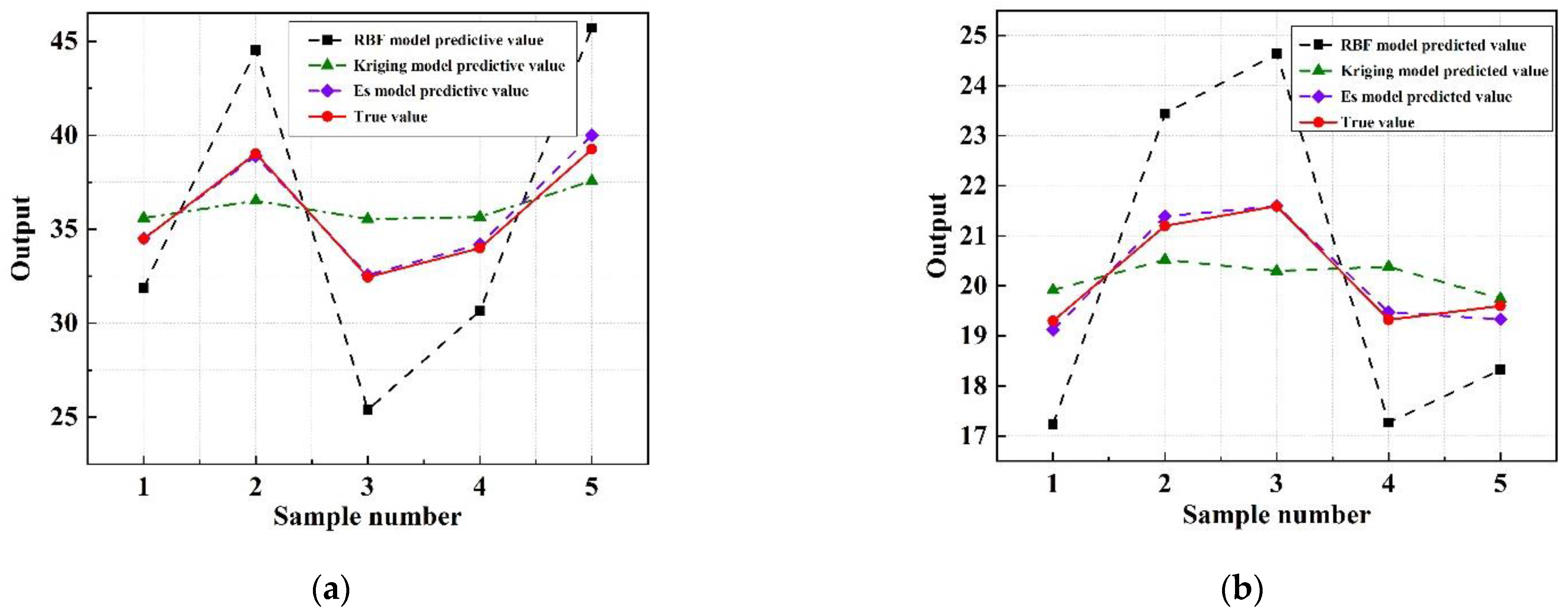
4.2. Ensemble of Surrogate Model

We built the sample space using optimal Latin hypercube sampling. In order to complete the fitting of the approximate model at a lower number of samples and form the response function of design variables and target parameters of the diagonal flow fan blades, an ensemble of surrogates model was formed by the combination of the radial basis function (RBF) and Kriging (KRG). The Ensemble of surrogates, also known as the weighted average surrogate model, is generally expressed as:

$${\widehat{y}}_e\left(x\right)={\displaystyle \sum _{i=1}^M{\omega }_i}\left(x\right){\widehat{y}}_i\left(x\right)$$

(10)

In the formula, ŷ_e(x) is the predicted value of the Ensemble of surrogates model; ŷ_i(x) and ω_i(x) are the predicted value and weight coefficient of the ith single model, respectively, and ${\displaystyle \sum _{i=1}^M{\omega }_i\left(x\right)}=1$.

First of all, the weight coefficient of a single model needs to be determined to construct an Ensemble of surrogates model. By assigning weights to each single model, the adverse effects of poor-performance models can be further reduced. The heuristic weight coefficient algorithm proposed by Goel et al. [17] is introduced here, and its operation formula is:

$$\begin{array}{l}{\omega }_i=\frac{{\omega }_i^{\ast }}{{\displaystyle \sum _{j=1}^n{\omega }_j^{\ast }}}\\ {\omega }_i^{\ast }={\left(E_i+\alpha E_{avg}\right)}^{\beta }\\ E_{avg}=\frac{{\displaystyle \sum _{j=1}^n{E}_j}}{n}\end{array}$$

(11)

where E_i is the generalized mean square error of the ith surrogate model, α (α < 1) controls the mean value of the surrogate model, β (β < 0) is used to adjust the influence of the single surrogate model on the Ensemble of surrogates model, and the recommended values are α = 0.05, β = −1.

We used the optimal Latin hypercube experimental design to obtain leaf sample space over a range of design variables. We set an appropriate number of training samples and test samples by considering the prediction accuracy of the approximate model and computation time cost. The root mean square error between the number of samples of different surrogate models and the corresponding output values is shown in

Table 1. Comparison of sample size and output response MSE for different surrogate models.

Delegation Model	Number of Training Samples	Efficiency MSE	MSE Flow MSE
RBF	40	50.183	12.542
RBF	50	40.127	10.229
RBF	60	34.982	7.732
RBF	70	28.212	4.908
Kriging	40	70.234	19.127
Kriging	50	35.235	8.394
Kriging	60	12.175	2.598
Kriging	70	4.536	0.740
ES	40	17.236	10.332
ES	50	4.556	3.194
ES	60	1.742	0.992
ES	70	0.125	0.032

.

Generally, there is a great relationship between the fitting accuracy of the surrogate model and the number of samples. More samples can ensure higher fitting accuracy. By comparing the prediction mean square error of the corresponding output values of different surrogate models under different training sample numbers, it can be seen that the fitting accuracy of the Kriging model increases with increasing sample size. The RBF model has obvious advantages in the lower number of samples. The Ensemble of surrogates model has the advantages of both models and has higher prediction accuracy under the same number of samples. Figure 9 shows the Ensemble of surrogates model’s test set error.

The model prediction deviations of the Kriging model, RBF model, and Ensemble of surrogates model under 70 training samples are shown in Figure 10. The mean square error MSE of each model under test samples (five groups) is selected to characterize the overall error.

It can be seen from the above figure that there is a big difference between the predicted value and the real value of RBF and Kriging models in terms of efficiency prediction and flow prediction, and the Ensemble of surrogates model has higher prediction accuracy than the above conventional prediction model. At the same time, in order to further intuitively evaluate the predictive ability of the Ensemble of surrogates model, the linear regression determination coefficient (R²) is introduced here.

$$R^2=1-\frac{{\displaystyle \sum _{i=1}^n{\left({\stackrel{⌢}{y}}_i-\overline{y}\right)}^2}}{{\displaystyle \sum _{i=1}^n{\left(y_i-\overline{y}\right)}^2}}$$

(12)

In the formula, i represents the sequence number, n is the number of all samples, $\overline{\mathrm{y}}$ is the average value of test samples, and ŷ is the predicted value of test samples. It is generally believed that when R² is close to 1, the fitting effect is better.

Table 2. Ensemble of surrogates model R².

	Qv	η
R2	0.973	0.966

shows the Ensemble of surrogates model R².

Figure 11 shows the optimization parameters and optimization variables efficiency flow under the Ensemble of surrogates model fitting surface.

4.3. Multi-Objective Optimization of Diagonal Flow Fan Blade

The NSGA-II algorithm is an efficient and fast sorting algorithm based on a genetic algorithm. It does not need any transformation of design objectives, and can achieve the purpose of screening individual advantages and disadvantages only according to the dominance relationship between individuals [18]. The algorithm uses the crowding distance evaluation method to replace the commonly used shared function method, so that it can control the distribution of individuals without determining a shared parameter. In this paper, four variables of CST parametric design are used to determine the maximum total pressure efficiency of the fan η_B and maximum flow q_v. The mathematical model of performance optimization of the diagonal flow fan is as follows:

$$\{\begin{array}{l}\max \left(q_v\left(v_0,v_1,v_2,v_3\right)\right)\\ \max \left({\eta }_B\left(v_0,v_1,v_2,v_3\right)\right)\\ 0.3\le v_0\le 0.7\\ 2\le v_1\le 4\\ 1\le v_2\le 3\\ 0.4\le v_3\le 0.8\end{array}$$

(13)

The Ensemble of surrogates model is solved by NSGA-II to obtain the Pareto solution set, as shown in Figure 12.

The Pareto frontier solution set obtained through optimization is shown in Figure 12. It can be seen that each solution set is relatively close. In engineering problems, there is a constraint relationship between some optimization target parameters. The improvement of one parameter target often leads to the decrease in another parameter index. Considering the flow improvement and efficiency of the diagonal flow fan, the efficiency maximization is sought under the flow requirement, and the optimization scheme of 0.5η_B + 0.5q_v is determined. Comparing the blades before and after optimization, it is found that under the design conditions, the effective air volume of the fan increases by 2.0 m³/min to 21.4 m³/min, and the total pressure efficiency increases by 2.8% to 38.9%.

Table 3. Parameters before and after arc optimization of diagonal flow fan blade.

Design Parameter	v0	v1	v2	v3
Original	0.417	3.074	1.779	0.551
Optimized	0.317	1.878	1.152	0.488

shows the comparison of parameters before and after arc optimization in the blade.

5. Numerical Simulation Analysis and Experimental Verification

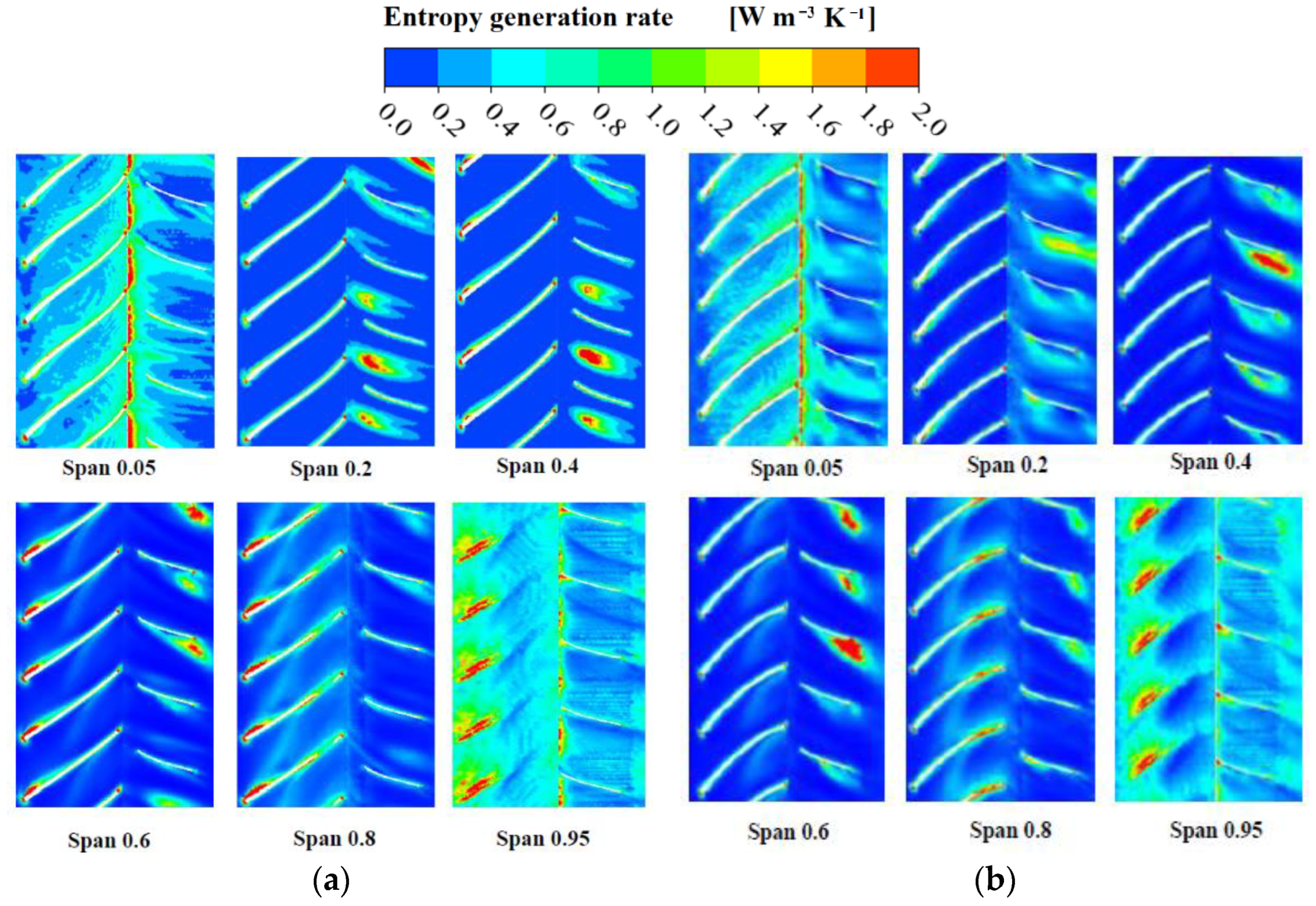
5.1. Energy Loss Analysis

In the process of the fan working on the fluid through the blade, due to the viscosity of the fluid medium and the existence of Reynolds stress, the irreversible process of the conversion of mechanical energy to internal energy occurs. So, there must be irreversible loss. Entropy generation theory [19,20] is introduced here to study the energy loss caused by viscous dissipation and turbulent dissipation in the fan before and after optimization from the perspective of thermodynamics. The viscous dissipative entropy generation and turbulent dissipative entropy generation can be obtained from the following equation. Figure 13 shows the specific definition of different blade height sections of the fan, and Figure 14 shows the entropy generation cloud diagram of different blade heights of the fan.

Viscous dissipation entropy generation is:

$${\dot{S}}_{\overline{D}}^{‴}=\frac{\mu }{T_{\mathrm{t}}}\left[{\left(\frac{\partial \overline{u}}{\partial y}+\frac{\partial \overline{v}}{\partial x}\right)}^2+{\left(\frac{\partial \overline{u}}{\partial z}+\frac{\partial \overline{w}}{\partial x}\right)}^2+{\left(\frac{\partial \overline{v}}{\partial z}+\frac{\partial \overline{w}}{\partial y}\right)}^2\right]+\frac{2\mu }{T_{\mathrm{t}}}\left[{\left(\frac{\partial \overline{u}}{\partial x}\right)}^2+{\left(\frac{\partial \overline{v}}{\partial y}\right)}^2+{\left(\frac{\partial \overline{w}}{\partial z}\right)}^2\right]$$

(14)

Turbulent dissipation entropy generation is:

$${\dot{S}}_{D^{\prime }}^{‴}=\frac{\mu }{T_{\mathrm{t}}}\left[{\left(\frac{\partial u^{\prime }}{\partial y}+\frac{\partial v^{\prime }}{\partial x}\right)}^2+{\left(\frac{\partial u^{\prime }}{\partial z}+\frac{\partial w^{\prime }}{\partial x}\right)}^2+{\left(\frac{\partial v^{\prime }}{\partial z}+\frac{\partial w^{\prime }}{\partial y}\right)}^2\right]+\frac{2\mu }{T_{\mathrm{t}}}\left[{\left(\frac{\partial u^{\prime }}{\partial x}\right)}^2+{\left(\frac{\partial v^{\prime }}{\partial y}\right)}^2+{\left(\frac{\partial w^{\prime }}{\partial z}\right)}^2\right]$$

(15)

where $\overline{\mathrm{u}}$, $\overline{\mathrm{v}}$, and $\overline{\mathrm{w}}$ are the components of average velocity in x, y, and z directions, m/s; u′, v′, and w′ are the components of pulsating velocity in x, y, and z directions, m/s; T_t is the temperature, K; and µ is hydrodynamic viscosity, Pa·s.

It can be seen from Figure 14 that the entropy generation of the blade part at the low blade height section (such as Span0.05, Span0.2, and Span0.4) mainly comes from the wake shedding, which will produce large unstable pressure pulsation, resulting in energy loss. At the high section of the middle blade (such as Span0.6 and Span0.8), blade loss caused by the incoming flow impact is gradually highlighted. The impact loss of the original impeller is more obvious, mainly in the leading edge area of the blade. The optimized impeller is due to the viscous effect of the airflow and the turbulent additional shear stress. At the high blade section (such as Span0.95), the tip leakage of the impeller is dominant, and there is no significant difference before and after optimization.

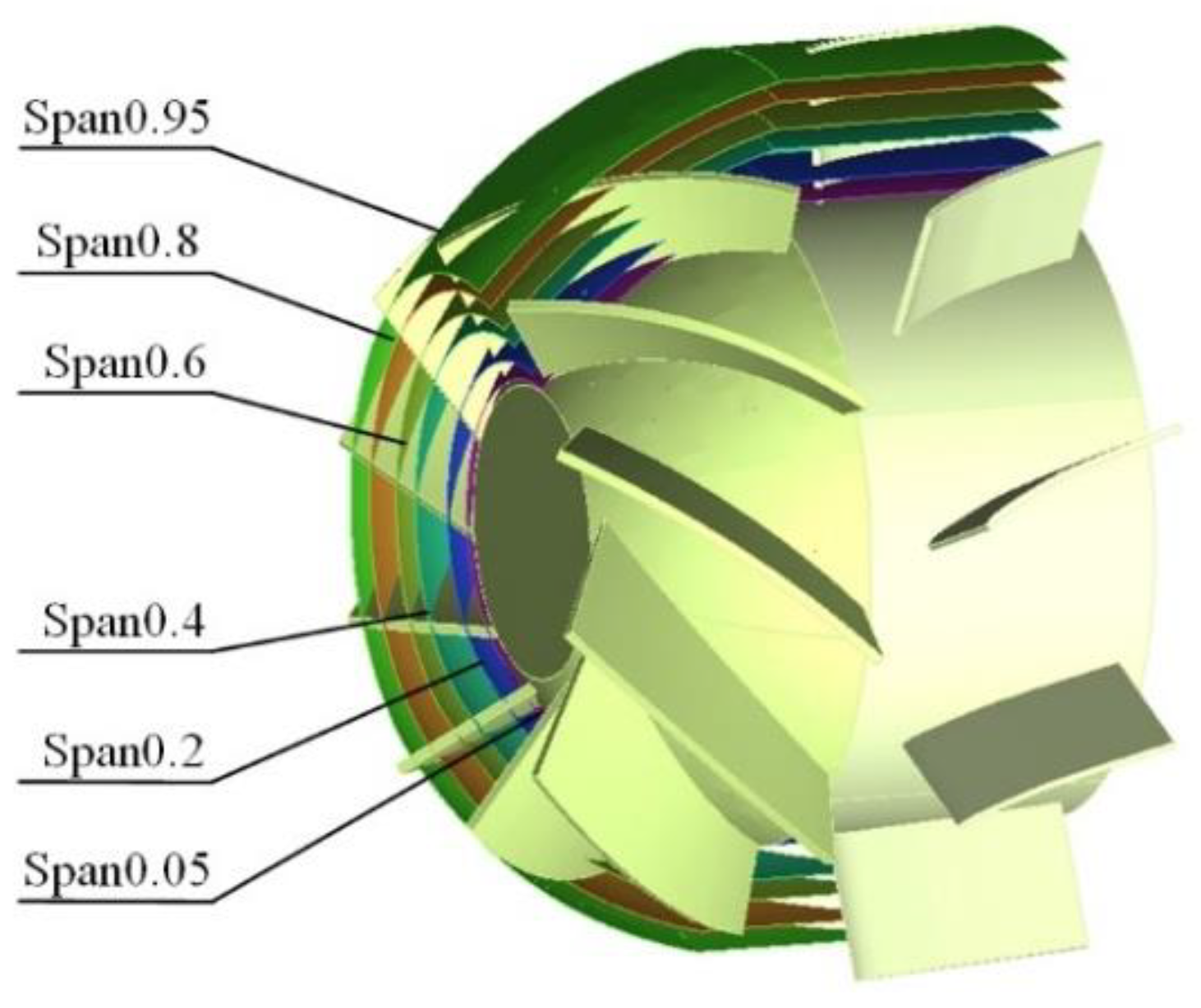
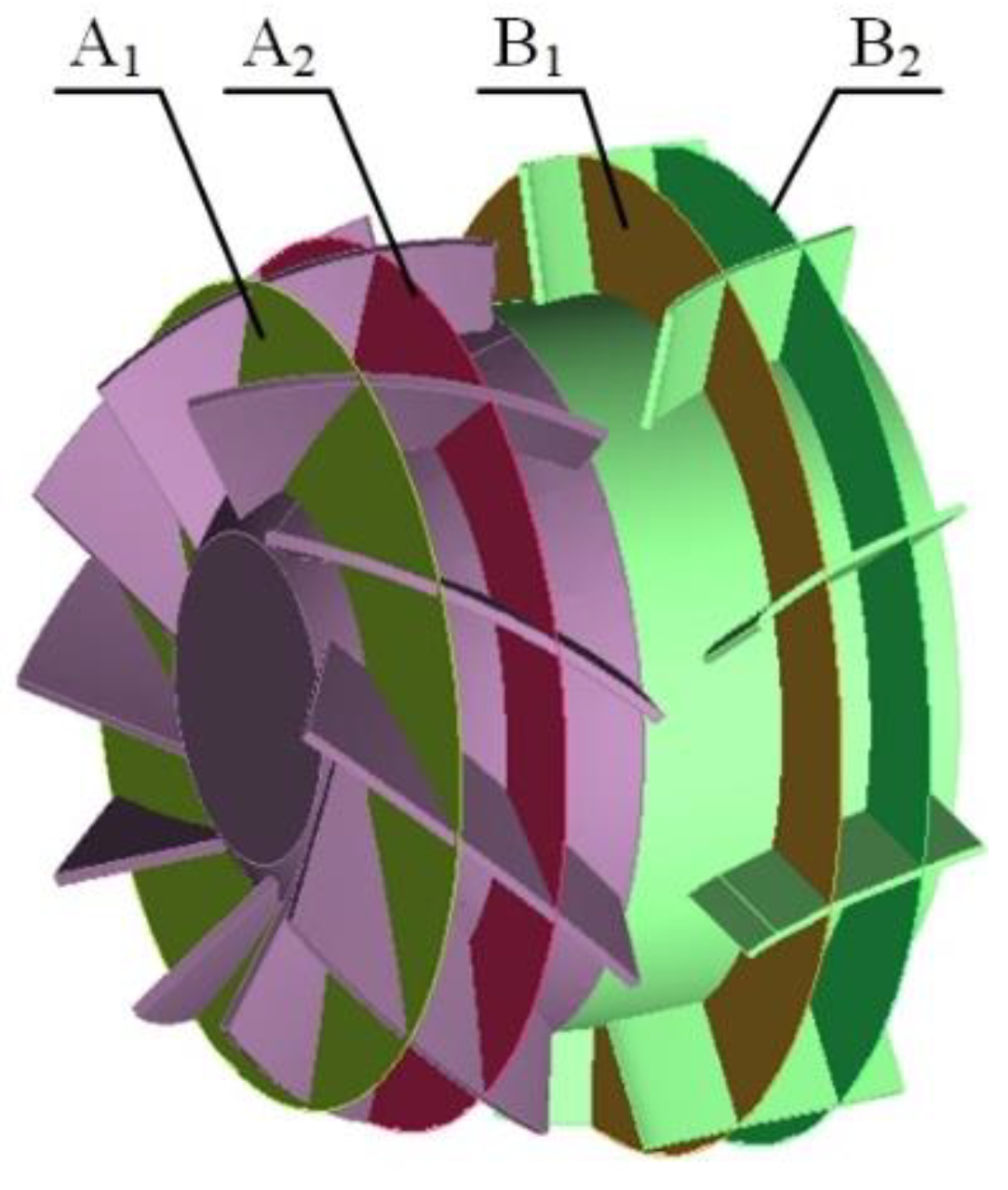
5.2. Internal Flow Analysis

The streamline distribution of the impeller before and after optimization is shown in Figure 15. When the incoming flow makes contact with the leading edge of the blade, the flow velocity increases rapidly due to the rotation of the impeller, and then decreases with the development of the blade passage. The high-speed range of the optimized impeller is obviously larger than that of the original impeller. The whole streamline is relatively flat, and there is no obvious bad flow area.

To further study the characteristics of internal flow, four planes are selected in the moving blade and guide vane basin along the direction of the medium flow to divide the basin equally. The sections selected on the impeller are A₁ and A₂, and the sections selected on the guide vane are B₁ and B₂, as shown in Figure 16.

The velocity distribution of each section is shown in Figure 17. Overall, the velocity changes, decreasing gradually along the airflow direction. After optimization, the airflow velocity in the impeller basin becomes significantly larger. The intuitive manifestation is that the fan flow rate is significantly improved, which is consistent with the previous optimization calculation results. At the same time, the velocity of the airflow in the guide vane basin is much lower than that in the blade basin. This is because the guide vane is a stationary component and cannot provide power. It only plays a role in changing the flow direction and diffusion. Therefore, a local low-speed zone appears near the guide vane wall.

Considering the cross-section shown in Figure 16, the pressure changes in the fan flow channel before and after optimization is shown in Figure 18.

Overall, globally, the static pressure of the impeller pressure surface is higher than that of suction surface; compared to the local guide vane channel of the guide vane, the pressure distribution of the local impeller channel of the impeller shows stronger periodicity. It is not difficult to find that the overall static pressure of the optimized guide vane is significantly higher than that before optimization. It is caused by the conversion of more kinetic energy into pressure energy. Therefore, the energy conversion ability of the optimized fan is improved.

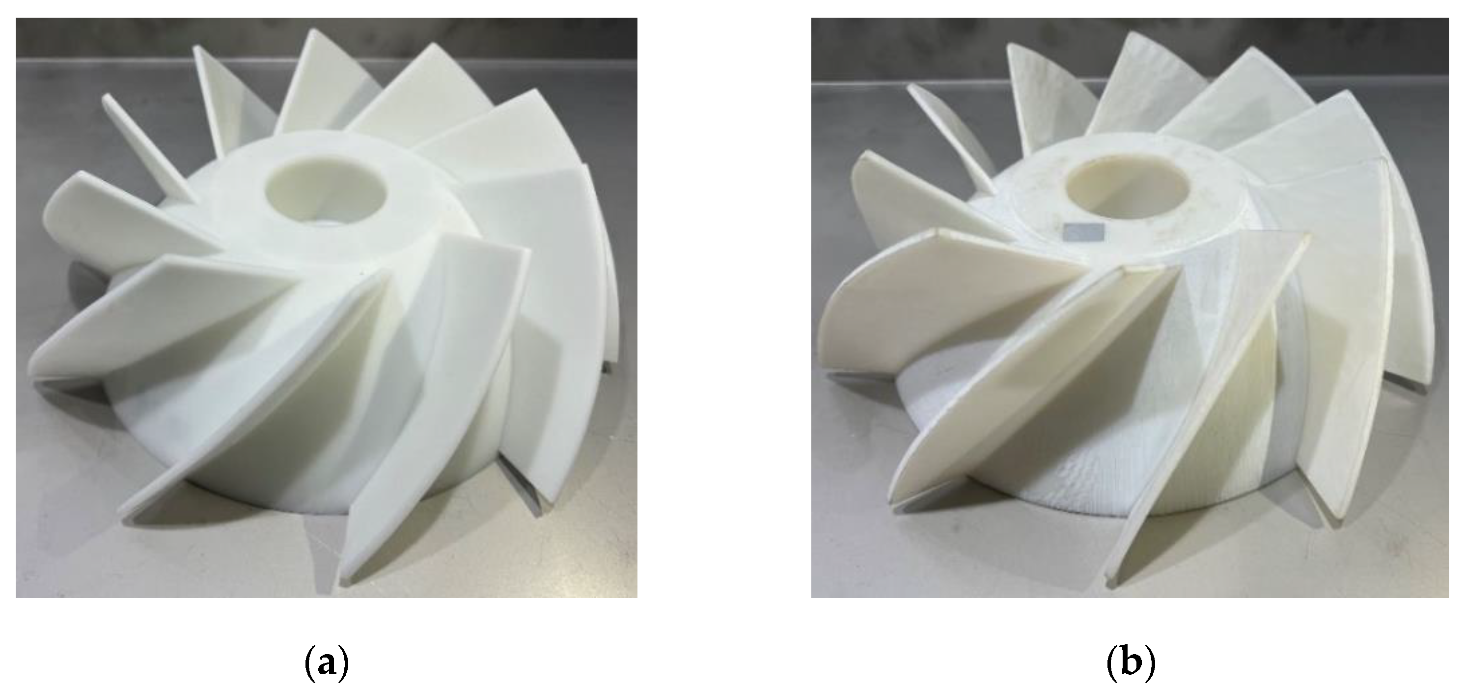
5.3. Experimental Verification

We determined the optimization of impeller by proofing to verify the performance of the optimized diagonal flow fan impeller. The impeller before and after optimization is shown in Figure 19. According to the regulations and requirements in ‘Fans—Performance testing using standardized airways (ISO 5801:2017)’ [13], its air performance was tested.

After the air performance test, the optimized and original fan performance curves were plotted on the same diagram to visually compare their performance changes, as shown in Figure 20.

Obviously, the optimized fan performance trends are basically consistent with the original. However, after impeller optimization, the fan had a higher total pressure efficiency when the flow rate was large, which is in line with the purpose of multi-objective optimization. When the optimized blade worked under the design condition, the fan air volume increased by 1.7 m³/min to 21.12 m³/min, and the total pressure efficiency increased by 3.2% to 38.9%. The test results are basically consistent with the optimized prediction results.

6. Conclusions

An Ensemble of surrogates model was established for the design parameters and response results of a small diagonal flow fan. The Pareto front of the Ensemble of surrogates model was solved by a fast non-dominated sorting algorithm to obtain the structural parameters of the wind turbine blades. Combined with numerical and experimental, the internal flow characteristics of the diagonal flow fan before and after modification were explored and studied. The following conclusions were obtained:

(1)

Based on the combination concept, a new Ensemble of surrogates model was generated by combining an RBF model and Kriging model, and the error was analyzed. It was verified that the prediction accuracy of the five test sets of the Ensemble of surrogates model is higher than that of the traditional model in terms of efficiency prediction and flow prediction, and its linear regression coefficient R² is close to 1, which further verifies that the Ensemble of surrogates model has higher prediction accuracy.

(2)

In this paper, the fast non-dominated sorting algorithm was used to optimize the flow rate and total pressure efficiency of the diagonal flow fan, which can greatly reduce the complexity of the calculation and has the characteristics of high accuracy in solving the Pareto solution set. The optimization work should not only focus on the flow rate of the diagonal flow fan, but also needs to pay attention to the efficiency (i.e., energy consumption). Therefore, this paper states that the weight relationship between the two optimization objectives should be considered comprehensively, and proposes a solution that uses the weighted objective function 0.5η_B + 0.5q_v to reach the maximum value.

(3)

Through the numerical simulation method, the flow characteristics of the diagonal flow fan before and after the modification are studied in depth. It is found that the optimized fan blade has stronger work performance, less energy loss, and significantly improved fan efficiency.

(4)

In order to further confirm the accuracy of the prediction method and optimization design, the optimized impeller was proofed and tested. The test results show that the optimized blade increased by 1.7 m³/min and the total pressure efficiency increased by 3.2% under the design condition of the fan.

References

1. Jia, L.; Tao, Z.; Wu, H.; Li, S.; Xing, S. Numerical Design and Optimization of the Rear Guide Vanes for a Tubular Mixed Flow Fan. Fan Technol. 2013, 1, 31–34. [Google Scholar]
2. Dong, W. Internal Flow Analysis on the Diagonal Fan and Retrofit Design for the Rotor. Master’s Thesis, Northwestern Polytechnical University, Xi’an, China, 2007. [Google Scholar]
3. Han, J. Research on Tonal Noise Characteristics and Noise Reduction Methods of Diagonal Flow Fan. Master’s Thesis, Zhejiang University, Hangzhou, China, 2021. [Google Scholar]
4. Hou, Z.; Yang, M.; Liang, X.; Wen, D. Numerical analysis and design optimization of diagonal flow fan for locomotives. Kongqi Donglixue Xuebao/Acta Aerodyn. Sin. 2018, 36, 300–306. [Google Scholar]
5. Ao, T.; Chen, J.; Cai, W. Analysis of flow loss in Impeller and Diffuser Oblique Flow Compressor. Mech. Manuf. Autom. 2022, 51, 61–64. [Google Scholar]
6. Furukawa, M.; Saiki, K.; Nagayoshi, K.; Kuroumaru, M.; Inoue, M. Effects of Stream Surface Inclination on Tip Leakage Flow Fields in Compressor Rotors. J. Turbomach. 1998, 120, 683–694. [Google Scholar] [CrossRef]
7. Jin, G.; Ouyang, H.; Du, C. Experimental investigation of extending stall-free mechanism of three-dimensional flow in circumferential skewed axial fans. Exp. Fluid Dyn. 2013, 27, 23–30. [Google Scholar]
8. Funakoshi, H.; Tsukamoto, H.; Miyazaki, K.; Miyagawa, K. Experimental study on unstable characteristics of mixed-flow pump at low flow-rates. In Proceedings of the ASME/JSME 2003 4th Joint Fluids Engineering Conference, Honolulu, HI, USA, 6–10 July 2003. [Google Scholar]
9. Li, Y.; Ouyang, H.; Du, Z.-H. Optimization Design and Experimental Study of Low-Pressure Axial Fan with Forward-Skewed Blades. Int. J. Rotating Mach. 2007, 2007, 85275. [Google Scholar]
10. Liu, Y.; Chen, L.; Shen, P.; Dai, R. Aero-Thermal Coupled Optimization of Turbine Cascade Endwall Based on Multi-surrogate Model. J. Eng. Thermophys. 2020, 41, 2942–2949. [Google Scholar]
11. Yang, K.; Zhou, S.; Hu, Y.; Zhou, H.; Jin, W. Energy Efficiency Optimization Design of a Forward-Swept Axial Flow Fan for Heat Pump. Front. Energy Res. 2021, 9, 700365. [Google Scholar] [CrossRef]
12. Wang, F. Computational Fluid Dynamics Analysis: Principle and Application of CFD Software; Tsinghua University Press: Beijing, China, 2004. [Google Scholar]
13. UNE-EN ISO 5801-2019; Fans-Performance Testing Using Standardized Airways (ISO 5801:2017). ISO Publishing: Geneve, Switzerland, 2019.
14. Zhou, S.; Hu, Y.; Lu, L.; Yang, K.; Gao, Z. IGV optimization for a large axial flow fan based on MRGP model and Sobol’ method. Front. Energy Res. 2022, 10, 823912. [Google Scholar] [CrossRef]
15. Kulfan, B.; Bussoletti, J. “Fundamental” Parameteric Geometry Representations for Aircraft Component Shapes. In Proceedings of the 11th AIAA/ISSMO Multidisciplinary Analysis and Optimization Conference, Portsmouth, VA, USA, 6–8 September 2006. [Google Scholar]
16. Kulfan, B.M. Universal Parametric Geometry Representation Method. J. Aircr. 2008, 45, 142–158. [Google Scholar] [CrossRef]
17. Goel, T.; Haftka, R.T.; Shyy, W.; Queipo, N.V. Ensemble of surrogates. Struct. Multidiscip. Optim. 2007, 33, 199–216. [Google Scholar] [CrossRef]
18. Wang, L.; Wang, T.; Luo, Y. Improved NSGA-II in Multi-Objective Optimization Studies of Wind Turbine Blades. Appl. Math. Mech. 2011, 32, 693–701. [Google Scholar] [CrossRef]
19. Wang, W.; Lin, Z.; Wang, J.; Li, Z. Optimization design of cascade profile based on entropy generation theory. J. Huazhong Univ. Sci. Technol. Nat. Sci. 2021, 49, 52–58. [Google Scholar]
20. Yang, F.; Li, Z.; Hu, W.; Liu, C.; Jiang, D.; Liu, D.; Nasr, A. Analysis of flow loss characteristics of slanted axial-flow pump device based on entropy production theory. R. Soc. Open Sci. 2022, 9, 211208. [Google Scholar] [CrossRef] [PubMed]
Figure 1. Physical model of small diagonal flow fan.
Applsci 12 09732 g001
Figure 2. Fan basin diagram.
Applsci 12 09732 g002
Figure 3. Grid model of diagonal flow fan. (a) Moving blade area grid. (b) Guide vane area grid.
Applsci 12 09732 g003
Figure 4. Grid independence verification.
Applsci 12 09732 g004
Figure 5. Air performance test. (a) Test device diagram (b) Field test diagram.
Applsci 12 09732 g005aApplsci 12 09732 g005b
Figure 6. Comparison of experimental and predicted values.
Applsci 12 09732 g006
Figure 7. Blades of diagonal flow fan and their parameterization. (a) Diagonal flow fan impeller. (b) Arc line in blade. (c) Blade parametric coordinates.
Applsci 12 09732 g007
Figure 8. Analysis of arc fitting error in blade.
Applsci 12 09732 g008
Figure 9. Ensemble of surrogates model test set test error.
Applsci 12 09732 g009
Figure 10. Prediction error of each model test set. (a) Efficiency prediction error of each model. (b) Flow prediction error of each model.
Applsci 12 09732 g010
Figure 11. Optimization parameters and optimization target fitting surface. (a) v0 and v1 fit surfaces with efficiency (%). (b) v2 and v3 Fitting surfaces with efficiency (%). (c) v0 and v1 fit surfaces with flow rate (m3/min). (d) v2 and v3 fit surfaces with flow rate (m3/min).
Applsci 12 09732 g011
Figure 12. Optimization objective Pareto frontier.
Applsci 12 09732 g012
Figure 13. Different leaf height sections.
Applsci 12 09732 g013
Figure 14. Cross-section entropy cloud diagram of different fan blade heights before and after optimization. (a) Original. (b) Optimized.
Applsci 12 09732 g014
Figure 15. Flow chart of impeller region. (a) Original. (b) Optimized.
Applsci 12 09732 g015
Figure 16. Cross-section of blade in different flow directions.
Applsci 12 09732 g016
Figure 17. Velocity distribution of different flow direction sections before and after optimization.
Applsci 12 09732 g017
Figure 18. Pressure distribution of different streamwise sections before and after optimization.
Applsci 12 09732 g018
Figure 19. Comparison diagram of impeller before and after optimization. (a) Original. (b) Optimized.
Applsci 12 09732 g019
Figure 20. Comparison of fan performance curves before and after optimization.
Applsci 12 09732 g020