Abstract
Generally, the results of imaging the limited view data in the inverse scattering problem are relatively poor, compared to those of imaging the full view data. It is known that solving this problem mathematically is very difficult. Therefore, the main purpose of this study is to solve the inverse scattering problem in the limited view situation for some cases by using artificial intelligence. Thus, we attempted to develop an artificial intelligence suitable for problem-solving for the cases where the number of scatterers was 2 and 3, respectively, based on CNN (Convolutional Neural Networks) and ANN (Artificial Neural Network) models. As a result, when the ReLU function was used as the activation function and ANN consisted of four hidden layers, a learning model with a small mean square error of the output data through the ground truth data and this learning model could be developed. In order to verify the performance and overfitting of the developed learning model, limited view data that were not used for learning were newly created. The mean square error between output data obtained from this and ground truth data was also small, and the data distributions between the two data were similar. In addition, the locations of scatterers by imaging the out data with the subspace migration algorithm could be accurately found. To support this, data related to artificial neural network learning and imaging results using the subspace migration algorithm are attached.
1. Introduction
An inverse problem refers to any problem related to finding the desired information using an indirect method such as observation when some information cannot be found directly in the field of mathematics or science. In other words, it indicates all problems related to obtaining the values of model parameters from observational data. This inverse problem has been widely used and studied not only in radiology but also in fields closely related to our lives, such as earth science, astronomy, engineering, and non-destructive inspection. Related works can be found in [1,2,3,4,5,6,7,8,9,10,11,12,13,14] and references therein.
The inverse scattering problem, which is one of the inverse problems, happens when electromagnetic waves whose information such as frequency or wavelength are known emitted into a scatterer included in the arbitrary space. Then, the problem is to find out the location, size, shape, and characteristics of the scatterers from the scattered waves. Although this inverse scattering problem is a significant field for research, it is known to be a difficult and complicated problem due to the fundamental nonlinearity and ill-posedness. Thus, no particular solutions have been developed other than a numerical method based on an iterative algorithm such as Newton’s method; refer to [15,16,17,18,19,20,21,22].
It is well-known that these iterative methods may not converge or may converge to a shape different from the ground truth unless a good initial value is given. In addition, although it converges to the desired shape, it may take a very long time. Therefore, there is a need for a non-iterative method that can directly obtain approximate information such as shape, location, etc., of a scatterer from the collected scattering wave despite the absence of an initial value. Motivated by this, various non-iterative methods have already been developed for the inverse scattering problem. Recently, the linear sampling method (LSM), which is based on the structure of the range of a self-adjoint operator, was developed and applied for determining the locations and shapes of unknown scatterers [23,24,25]. However, the LSM requires a large number of directions of the incident and corresponding scattered fields, and most of the research deals with the full-view inverse scattering problem. MUltiple SIgnal Classification (MUSIC), which is a method of characterizing the range of a self-adjoint operator (see [26] for instance), is also applied to various inverse scattering problems and microwave imaging [27,28,29]. Let us mention that the location of small scatterers can be identified clearly through the MUSIC in the full-view problem, but, in the limited-view problem, incorrect locations are retrieved, refer to [30]. Moreover, similar to the LSM, MUSIC requires a significant number of directions of the incident and scattered field data. Direct and orthogonality sampling methods are fast, effective, and robust techniques for retrieving small scatterers with single source [31,32,33], but the imaging performance is significantly dependent on the location of source or direction of incident field. Moreover, similar to the MUSIC, incorrect locations of small scatterers are retrieved in a limited-view inverse scattering problem. Topological derivative (TD) based imaging techniques have been successfully applied to various inverse scattering problems [34,35,36]. One of the advantages of the TD is that one can obtain good results even with a small number of incident field data, but most of research is applied to the full-view inverse scattering problem.
As shown above, the inverse scattering problem can be divided into a full-view situation and a limited-view situation. We refer to Figure 1 for an illustration of the full- and limited-view inverse scattering problems. In situation such as exploring the ground, only limited-view data can be collected, so research on the limited-view situation is required. In a limited-view situation, imaging is possible with the aforementioned algorithms, but the imaging performance is very poor compared to when full-view data are given. Therefore, research has been constantly conducted to solve this problem. Some research presented mathematical analyses of non-repetitive imaging algorithms performed when limited-view data are given (see [37,38,39,40,41,42,43,44,45,46] for instance). However, compared to the studies on the non-iterative imaging techniques in the full-view situation, there have been few studies in the limited-view situation.
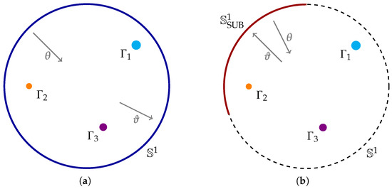
Figure 1.
Schematic diagram of full- and limited-view inverse scattering problems. (a) Full-view situation; (b) Limited-view situation.
Therefore, in this study, in order to improve the imaging performance in the limited-view problem, the artificial neural network model was developed that outputs the corresponding full-view data when the limited-view data are input for the case of two and three scatterers. For this purpose, the artificial neural network learned artificial neural network in various ways using the data generated for each case. Consequently, a learning model in which the mean square error between the output data from the artificial neural network and the actual data are not large can be developed.
For the purpose of verifying the effectiveness of the output data drawn from the artificial neural network, it was confirmed that the ground truth data and the imaging result were very similar as a result of imaging the output data several times using the subspace migration algorithm. In this way, it was confirmed that artificial neural networks can be used importantly to solve the inverse scattering problem.
This paper is organized as follows. In Section 2, we briefly introduce the basic concept of the two-dimensional direct scattering problems in the presence of small scatterers located in a homogeneous space and subspace migration imaging technique from the generated multi-static response (MSR) matrix whose elements are measured in the far-field pattern. In Section 3, we design an adopted artificial neural network model for generating complete elements of the MSR matrix and corresponding training results. The models developed for the case of two scatterers and three scatterers are described respectively. In Section 4, we exhibit various numerical simulation results to show the pros and cons of the designed artificial neural network. Finally, a short conclusion including an outline of future work is provided in Section 5.
2. Direct Scattering Problem and Subspace Migration
2.1. Two-Dimensional Direct Scattering Problem and Far-Field Pattern
Here, we briefly introduce a basic concept of the two-dimensional direct scattering problem in the presence of a set of small scatterers and the imaging function of subspace migration. Throughout this paper, we denote , , being a small scatterer embedded in the two-dimensional homogeneous space and being the collection of . For this purpose, we assume that every is a small ball with radius and location .
Here, we assume that and are completely characterized by their dielectric permittivity at a given angular frequency , where f denotes the ordinary frequency. Let and denote the permittivity of the and , respectively. Correspondingly, we can introduce the following piecewise constant of permittivity
With this, we denote as the background wavenumber. Here, is the value of magnetic permeability.
Here, we consider the plane-wave illumination: as the given incident field with the propagation direction that satisfies the following Helmholtz equation
Here, denotes the unit circle centered at the origin in . With this, we denote as the time-harmonic total field which satisfies the Helmholtz equation
with transmission condition on the boundaries of , . Usually, the can be split into the incident field and the scattered field , which satisfies the Sommerfeld radiation condition
Let be the far-field pattern corresponding to the scattered field with observation direction that satisfies
Based on [47], the far-field pattern can be represented as an asymptotic expansion formula
2.2. Subspace Migration Imaging Algorithm
Here, we apply the (1) to introduce the subspace migration algorithm for a direct imaging of from collected far-field pattern data
where denotes a connected, proper subset of (see Figure 1). With this, we generate the following MSR matrix such that
Based on the (1), each element can be written as
Based on the above representation, we introduce the following unit vector: for each ,
Then, can be decomposed as follows:
The imaging function of the subspace migration can be introduced based on the above decomposition. To this end, we perform the singular value decomposition of :
where denotes the nth singular value, and are the nth left- and right-singular vectors of , respectively. Since the following relation already be examined in [48]
we can introduce the following imaging function: for each
Here, . Then, when and when so that the location can be identified through the map of .
It is worth mentioning that subspace migration can be applied to the full- and limited-view inverse scattering problems. However, one cannot retrieve good results in the limited-view problem when total number N is small, while good results can be guaranteed in a full-view problem. A theoretical reason is as follows. Refer to [43]:
Theorem 1.
Let and . Then, for sufficiently large N and k, can be represented as
where the term , which degrades the imaging performance, is given by
Notice that, in the full-view problem, the range of incident and observation directions is so that the term can be removed. This means that the scatterers can be retrieved via the map of in a full-view problem. Therefore, for a proper identification of scatterers, it is natural to consider the generation of complete elements of MSR matrix from limited-view data. Unfortunately, one needs prior information of scatterers to generate missing elements so that direct generation of the elements is very difficult.
Motivated by this difficulty, we consider the generation of the MSR matrix in a full-view configuration from the MSR matrix in a limited-view configuration: for an even number N, generate complete elements , of from the following MSR matrix :
3. Artificial Neural Network Model and Training Results
It was thought that it would be difficult to train an artificial neural network when the number of scatterers was varied, so two learning models were developed for each case of two and three scatterers. For learning, we apply incident and observation directions for full-view data such that
Throughout this paper, we assume that there exist 2 or 3 scatterers with the same radii and permittivities . For a limited-view situation, we apply first incident and observation directions . With this setting, the far-field pattern data of at wavenumber was generated by solving the Foldy–Lax formulation (see [49], for instance). Therefore, values of the MSR matrix of full-view data are partitioned into four data groups as shown in Figure 2, and then data preprocessing is performed to convert group 1 data into input data.
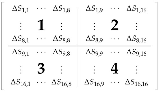
Figure 2.
Partitioning of the MSR matrix.
Then, three training data sets were created using the data of groups 2, 3, and 4 as the correct label, and then three artificial neural networks were trained using each data. That is, in the first artificial neural network, the data of groups 1 and 2 are training data sets, in the second artificial neural network, the data of groups 1 and 3 are training data sets, and in the third artificial neural network, the data of groups 1 and 4 are used as training data sets, which were applied to each artificial neural network as a training data set.
In order to find a suitable learning model to solve the problem of constructing full view data from limited view data, the number of layers and the number of nodes of hidden layers were adjusted in CNN and ANN models, and experiments were conducted using various activation functions. In the CNN model. a suitable model could not be found. However, when the ReLU function was used as the activation function in the ANN model and the number of hidden layers was 3, a learning model with a small mean square error could be found. In order to solve the overfitting problem, which is the major problem of ANN, we proceeded the learning. Even though the mean square error of the training data decreased, the mean square error of the test data did not show increase or decrease. In this case, we proceeded the learning process trying another model or increased the amount of training data. In addition, in order to reduce the complexity of the model, the number of hidden layers and the frequency of learning were adjusted to be as small as possible. In order to increase the learning rate and apply the ReLU function, the data cleansing of resulted in . Then, the data output through the artificial neural network, , was converted to by performing data preprocessing, and the final output was made.
The artificial neural network model was constructed to generate three data using limited-view data as shown in Figure 3, and the artificial neural network consists of an input layer and three hidden layers and an output layer. Activation function used ReLU, and optimization algorithm used Adam, and data were preprocessed into data, to be an input into the artificial neural network. and inputting three different artificial neural networks, and made them learned [50,51,52,53,54]. By processing three output data drawn from each artificial neural network and using data used for input, data became a final output.
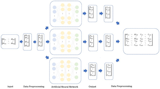
Figure 3.
Schematic diagram of an artificial neural network.
3.1. The Case of Having Two Scatterers
When the number of scatterers is 2, after generating 10,000 full-view data for artificial neural network learning and testing, 9500 of them were divided into training data set and 500 are divided into test data set to proceed the learning. That is, the ratio of training data and test data were set to 95:5. Each time the artificial neural network was trained five times, the mean square error between the output data from each artificial neural network and the ground truth data were measured and graphed as shown in Figure 4a–c In this case, the x-axis is the number of learning, the red line is the mean square error for the validation data, and the green line is the mean square error for the training data. As shown in the figure, it can be seen that the mean square error measured using the training data and the validation data are similar as the learning progressed in the three artificial neural networks. As a result of calculating the mean square error with 500 test data after the learning was finished, as shown in Figure 4d, about 88% is distributed between 0 and 0.02, and the error is found to be very small because the maximum error is 0.07.
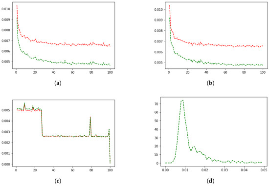
Figure 4.
Cases with two scatterers, Mean square error (a–c) for each group of test data and distribution of mean square error of test data (d).
In addition, to identify the similarity between the ground truth data and the output data obtained through the trained model, using the image map (imshow) function of Python, output data were separated into the real-part and imaginary-part to be visualized, respectively, like Figure 5. Looking at the figure, it can be seen that the distribution patterns of the two data are similar to each other. That is, since the error between the ground truth data and the output data through the learned model is small and the distribution pattern is similar, it can be predicted that the results obtained by imaging using the two data will be similar.
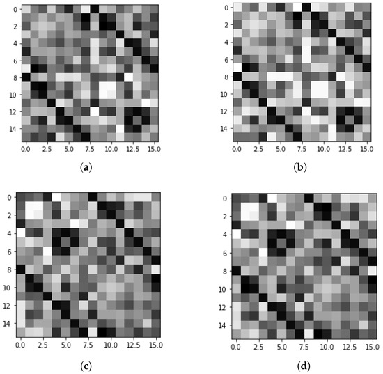
Figure 5.
Visualization of the real-part and imaginary-part of ground truth data and output data when there are two scatterers. (a) ground truth data (real-part); (b) output data (real-part); (c) ground truth data (imaginary-part); (d) output data (imaginary-part).
3.2. The Case of Having Three Scatterers
In the case of three scatterers, 10,000 data were generated and learned in the same way as in the case of two scatterers, but the results were not good. Thus, 110,000 data were newly created, and the learning was performed again by using 99,500 training data, 500 validation data, and 10,000 test data set. That is, learning was carried out by dividing the ratio of training data and test data by 10:1. As before, every time the artificial neural network is trained five times, the mean square error of the output value from each artificial neural network and the actual value is measured and graphed with each group, as shown in Figure 6a–c. As shown in Figure 6, it can be seen that the mean square error measured using the training data and the validation data are similar when learning is performed in three artificial neural networks.
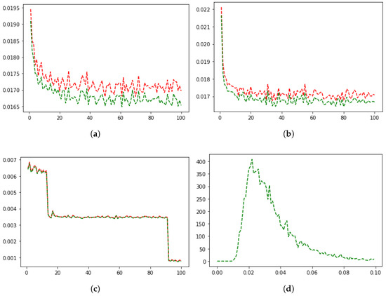
Figure 6.
Cases with three scatterers, Mean square error (a–c) for each group of test data and distribution of mean square error of test data (d).
Looking at this result alone, it can be seen that there is little error in the third artificial neural network, and the error in the first artificial neural network is relatively large. Through this, it can be deduced that group 1 and group 4 may have a higher mathematical correlation than other groups.
In order to more objectively check whether the learning was successfully carried out, the mean square error between the output data and the ground truth data were calculated using 10,000 test data that were not used for learning at all. As a result, as shown in Figure 5d, the mean square error for more than 70% of the test data was less than 0.04, the largest error was 0.166, and the smallest error was 0.01.
In addition, in order to understand the similarity between the ground truth data and the output data through the trained model, as in the previous case, the real-part and the imaginary-part were visualized for randomly generated data, respectively. As shown in Figure 7, it can be seen that the distribution patterns of the two data are similar to each other. That is, in this case as well, it can be predicted that the imaging results obtained by using the two data will be similar.
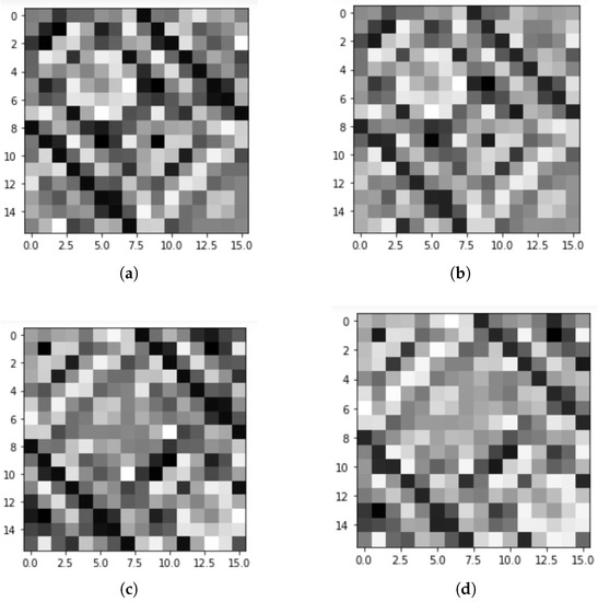
Figure 7.
Visualization of real-part and imaginary-part of ground truth data and output data when there are three scatterers. (a) ground truth data (real-part); (b) output data (real-part); (c) ground truth data (imaginary-part); (d) output data (imaginary-part).
4. Results of Numerical Simulations and Conclusions
In order to check whether the learning of the artificial neural network was properly carried out as desired, the MSR matrix was created with input data, output data, and ground truth data. In addition, then using the subspace migration algorithm, imaging was performed for two and three scatterers, respectively.
4.1. The Case of Having Two Scatterers
First, in the case of having two scatterers, the results of imaging with the subspace migration algorithm using the output data by inputting the test data of No. 1, No. 400, and No. 500 into the developed model and ground truth data are shown in Figure 8. The parts highlighted in red in this figure are the locations of the scatterers. As a result of imaging with ground truth data and learning data in all three cases, it can be seen that the locations of the scatterers are the same.
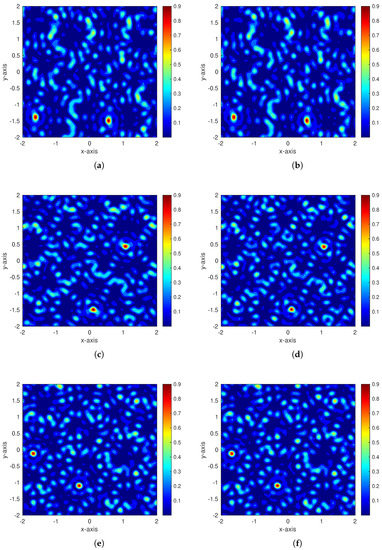
Figure 8.
Imaging results for ground truth data and learning data with two scatterers. (a) true data No. 1; (b) learning data No. 1; (c) true data No. 400; (d) learning data No. 400; (e) true data No. 500; (f) learning data No. 500.
In addition, in order to check whether the learning was successfully performed, we recreated the data. The imaging result of this recreated data using the subspace migration algorithm and the imaging result of the output data obtained by inputting this data into the learning model and the distributions of its singular values are shown in Figure 9. In this figure, the results of imaging the ground truth data and the output data show that there is little difference in the afterimages and the locations of the scatterers between two images. In addition, when (a) and (c) are compared, although the distributions of singular values are somewhat different, there is no problem in finding the locations of the scatterers because the two singular values are relatively large.
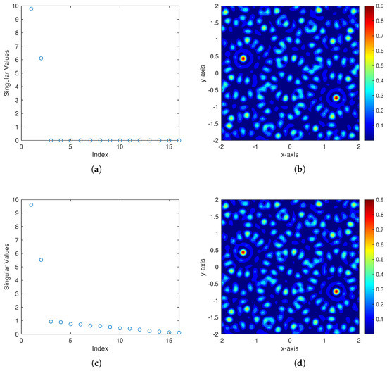
Figure 9.
Singular value distribution and imaging results for randomly generated scatter’s data. (a) SVD with true data; (b) imaging result with true data; (c) SVD with learning data; (d) imaging result with learning data.
In addition, referring to Figure 10, as shown in (a), the difference between singular values is relatively small, so, as a result of imaging limited view data, it may not be possible to locate the scatterers as in (b). When the singular value is calculated with the full view data output by inputting this limited view data into the learning model, there are two points with relatively large singular values as shown in (c). The locations of the scatterers can be easily found as shown in the imaging result (d). To sum up, it can be seen that, if the number of scatterers is two, the developed artificial neural network model constructs the correct full view data from the limited view data well.
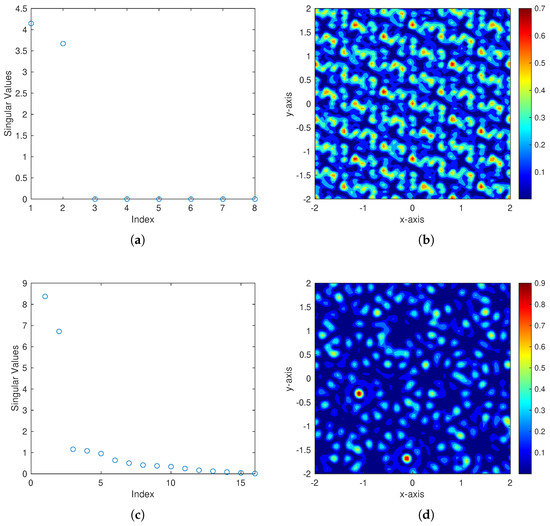
Figure 10.
Singular value distribution and imaging result of limited-view data (top) and output data (bottom). (a) SVD with limited-view data; (b) imaging result with true data; (c) SVD with full-view data; (d) imaging result with learning data.
4.2. The Case of Having Three Scatterers
In the case of three scatterers, as a result of learning 10,000 data, three high singular values were found as shown in Figure 11, but it can be seen that it is difficult to specify the location of the scatterers due to poor imaging results. Since further learning may lead to a risk of overfitting, the amount of data used for learning was increased.
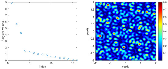
Figure 11.
Singular value distribution and imaging results for output data from a model learned with 10,000 data.
Therefore, 100,000 data were newly created and learned again, and the previously generated 10,000 data were not used for learning but used as test data. In order to confirm that the learning progressed well, among the output full view data from the test data input into the learning model, the cases with the largest and smallest mean square errors, compared to the ground truth data, are imaged with the subspace migration algorithm in Figure 12 and Figure 13, respectively. In both cases, when imaged with ground truth data (Figure 12a and Figure 13a) and data output through the learning model (Figure 12b and Figure 13b), it can be seen that the positions of the three scatterers highlighted in red are the same. In addition, it can be seen that, when a singular value is calculated using this data, three relatively large singular values are detected. Therefore, it can be considered that the full view data are well constructed from the limited view data, unlike when the artificial neural network is trained using 10,000 data.
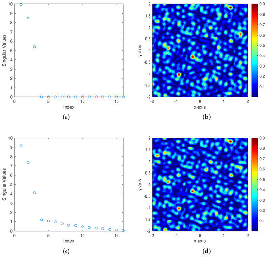
Figure 12.
Singular value distribution and imaging results for the case with the largest mean square error case among the test data. (a) SVD with true data; (b) imaging result with true data; (c) SVD with learning data; (d) imaging result with learning data.
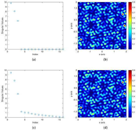
Figure 13.
Singular value distribution and imaging results for the case with the smallest mean square error case among the test data. (a) SVD with true data; (b) imaging result with true data; (c) SVD with learning data; (d) imaging result with learning data.
In addition, as in the case of two scatterers, the results of imaging the ground truth data of randomly generated scatterers and the data output by inputting this data into the learning model and the distribution of the singular value are shown in Figure 14. At this time, there are three points with large singular values in (a), (c), and (e), but in the case of limited view data, the three singular values are smaller than in other cases, so, when imaging, the location of the scatterers could not be found as shown in (b). However, when imaging with full view data output from the learning model, the locations of the scatterers could be found as shown in (f), and it was similar to the imaging result with actual ground truth data in (d). In other words, when arbitrary data that was not used at all for learning was input and imaged as output data, the locations of the scatterers could be found well. Therefore, even though the number of scatterers is three, it can be confirmed that the developed artificial neural network model has been successfully trained to construct the full-view data from the limited-view data input.
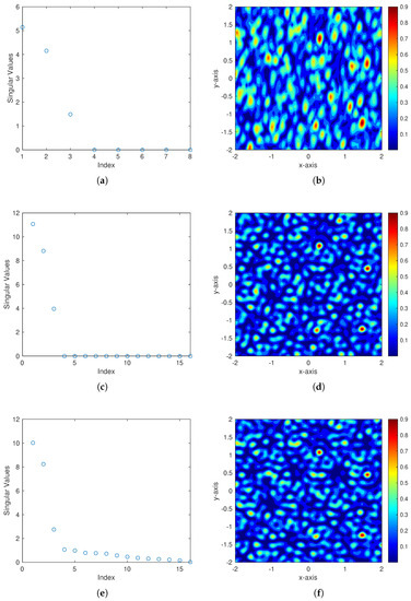
Figure 14.
Imaging result and singular value distribution for limited view data (top), ground truth data (middle), output data (bottom). (a) SVD with limited-view data; (b) imaging result with limited view data; (c) SVD with true data; (d) imaging result with true data; (e) SVD with learning data; (f) imaging result with learning data.
The fundamental problem with the inverse scattering problem in limited view situations is that it is sometimes impossible to locate the scatterers when imaging with limited view data due to insufficient data. Through previous experiments, it was found that this problem can be solved to some extent using artificial intelligence. Based on this study, we can draw the following conclusions.
- (i)
- For the cases of two and three scatterers, it is possible to develop a learning model that constructs the full view data from the limited view data with a small mean square error and similar data distribution compared to the ground truth data. In addition, the distributions of singular values calculated from the data output from the developed model or the results of imaging with the subspace migration algorithm were similar to the ground truth data, so the locations of the scatterers could be found.
- (ii)
- (iii)
- As shown in Figure 15, the error distribution of ground truth data and full view data output from the developed model shows that the error between group 1 and group 4 is relatively small. Since the full view data output from this learning model is from the limited view data of group 1, it can be seen that the correlation between the data of group 1 and the data of group 4 is high.
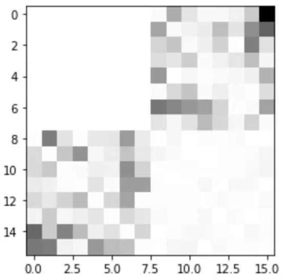 Figure 15. Error distribution between ground truth data and output data (the darker the color, the greater the error).
 - (iv)
- (v)
- Attempts to solve the inverse scattering problem using artificial intelligence mainly used the image for training. However, this study shows that it can be efficient to use data collected from transmission and receiving antennas directly for training artificial intelligence.
5. Discussion
From the above conclusions, future research topics can be considered. First, in this study, a learning model was developed separately for the cases of two and three scatterers, but we plan to develop it as one model in the future. Furthermore, we try to develop a model applicable to limited view data for an arbitrary number of scatterers. Second, it can be expected that the phenomena of conclusions 4 and 5 can be analyzed mathematically. Since mathematical analyses of several imaging functions have already been performed, it can be said to be a highly feasible research topic [55,56]. Finally, the method of directly using the data collected from the transmission and receiving antennas used in this study for artificial intelligence training can be applied to a wider variety of inverse problems. In real life, for example, data of diagonal components cannot be collected in the MSR matrix due to the limitations of the technology. Therefore, in the past, diagonal components were often set to 0 or 1, collectively. However, it is expected that the method used in this study will be used to develop a learning model that provides more appropriate diagonal components.
Author Contributions
Conceptualization, S.-S.J., W.-K.P. and Y.-D.J.; methodology, Y.-D.J.; software, S.-S.J., W.-K.P. and Y.-D.J.; validation, S.-S.J., W.-K.P. and Y.-D.J.; formal analysis, W.-K.P. and Y.-D.J.; investigation, S.-S.J., W.-K.P. and Y.-D.J.; data curation, S.-S.J. and W.-K.P.; writing—original draft preparation, Y.-D.J.; writing—review and editing, S.-S.J., W.-K.P. and Y.-D.J.; visualization, S.-S.J., W.-K.P. and Y.-D.J.; supervision, Y.-D.J.; project administration, Y.-D.J.; funding acquisition, W.-K.P. All authors have read and agreed to the published version of the manuscript.
Funding
This research was supported by the National Research Foundation of Korea (NRF) grant funded by the Korean government (MSIT) (NRF-2020R1A2C1A01005221) and the research program of Kookmin University.
Conflicts of Interest
The authors declare no conflict of interest.
References
- Acharya, R.; Wasserman, R.; Stevens, J.; Hinojosa, C. Biomedical imaging modalities: A tutorial. Comput. Med. Imaging Graph. 1995, 19, 3–25. [Google Scholar] [CrossRef]
- Ammari, H. An Introduction to Mathematics of Emerging Biomedical Imaging; Mathematics and Applications Series; Springer: Berlin, Germany, 2008; Volume 62. [Google Scholar]
- Ammari, H.; Bretin, E.; Garnier, J.; Kang, H.; Lee, H.; Wahab, A. Mathematical Methods in Elasticity Imaging; Princeton Series in Applied Mathematics; Princeton University Press: Princeton, NJ, USA, 2015. [Google Scholar]
- Arridge, S. Optical tomography in medical imaging. Inverse Prob. 1999, 15, R41–R93. [Google Scholar] [CrossRef]
- Bleistein, N.; Cohen, J.; Stockwell, J.S., Jr. Mathematics of Multidimensional Seismic Imaging, Migration, and Inversion; Springer: New York, NY, USA, 2001. [Google Scholar]
- Borcea, L. Electrical Impedance Tomography. Inverse Prob. 2002, 18, R99–R136. [Google Scholar] [CrossRef]
- Chandra, R.; Zhou, H.; Balasingham, I.; Narayanan, R.M. On the opportunities and challenges in microwave medical sensing and imaging. IEEE Trans. Biomed. Eng. 2015, 62, 1667–1682. [Google Scholar] [CrossRef]
- Cheney, M.; Issacson, D.; Newell, J.C. Electrical Impedance Tomography. SIAM Rev. 1999, 41, 85–101. [Google Scholar] [CrossRef]
- Chernyak, V.S. Fundamentals of Multisite Radar Systems: Multistatic Radars and Multiradar Systems; CRC Press: Boca Raton, FL, USA, 1998. [Google Scholar]
- Colton, D.; Kress, R. Inverse Acoustic and Electromagnetic Scattering Problems; Mathematics and Applications Series; Springer: New York, NY, USA, 1998. [Google Scholar]
- Dorn, O.; Lesselier, D. Level set methods for inverse scattering. Inverse Prob. 2006, 22, R67–R131. [Google Scholar] [CrossRef]
- Obeidat, H.; Shuaieb, W.; Obeidat, O.; Abd-Alhameed, R. A review of indoor localization techniques and wireless technologies. Wirel. Pers. Commun. 2021, 119, 289–327. [Google Scholar] [CrossRef]
- Seo, J.K.; Woo, E.J. Magnetic resonance electrical impedance tomography (MREIT). SIAM Rev. 2011, 53, 40–68. [Google Scholar] [CrossRef]
- Zhdanov, M.S. Geophysical Inverse Theory and Regularization Problems; Elsevier: Amsterdam, The Netherlands, 2002. [Google Scholar]
- Ahmad, S.; Strauss, T.; Kupis, S.; Khan, T. Comparison of statistical inversion with iteratively regularized Gauss Newton method for image reconstruction in electrical impedance tomography. Appl. Math. Comput. 2019, 358, 436–448. [Google Scholar] [CrossRef]
- Ferreira, A.D.; Novotny, A.A. A new non-iterative reconstruction method for the electrical impedance tomography problem. Inverse Prob. 2017, 33, 35005. [Google Scholar] [CrossRef]
- Kristensen, P.K.; Martinez-Panedab, E. Phase field fracture modelling using quasi-Newton methods and a new adaptive step scheme. Theor. Appl. Fract. Mec. 2020, 107, 102446. [Google Scholar] [CrossRef]
- Liu, Z. A new scheme based on Born iterative method for solving inverse scattering problems with noise disturbance. IEEE Geosci. Remote Sens. Lett. 2019, 16, 1021–1025. [Google Scholar] [CrossRef]
- Proinov, P.D. New general convergence theory for iterative processes and its applications to Newton–Kantorovich type theorems. J. Complex. 2010, 26, 3–42. [Google Scholar] [CrossRef]
- Souvorov, A.E.; Bulyshev, A.E.; Semenov, S.Y.; Svenson, R.H.; Nazarov, A.G.; Sizov, Y.E.; Tatsis, G.P. Microwave tomography: A two-dimensional Newton iterative scheme. IEEE Trans. Microwave Theory Tech. 1998, 46, 1654–1659. [Google Scholar] [CrossRef]
- Timonov, A.; Klibanov, M.V. A new iterative procedure for the numerical solution of coefficient inverse problems. Appl. Numer. Math. 2005, 55, 191–203. [Google Scholar] [CrossRef]
- Wick, T. Modified Newton methods for solving fully monolithic phase-field quasi-static brittle fracture propagation. Comput. Meth. Appl. Mech. Eng. 2017, 325, 577–611. [Google Scholar] [CrossRef]
- Aram, M.G.; Haghparast, M.; Abrishamian, M.S.; Mirtaheri, A. Comparison of imaging quality between linear sampling method and time reversal in microwave imaging problems. Inverse Probl. Sci. Eng. 2016, 24, 1347–1363. [Google Scholar] [CrossRef]
- Alqadah, H.F.; Valdivia, N. A frequency based constraint for a multi-frequency linear sampling method. Inverse Prob. 2013, 29, 95019. [Google Scholar] [CrossRef]
- Colton, D.; Haddar, H.; Monk, P. The linear sampling method for solving the electromagnetic inverse scattering problem. SIAM J. Sci. Comput. 2002, 24, 719–731. [Google Scholar] [CrossRef]
- Cheney, M. The linear sampling method and the MUSIC algorithm. Inverse Prob. 2001, 17, 591–595. [Google Scholar] [CrossRef]
- Park, W.K. Asymptotic properties of MUSIC-type imaging in two-dimensional inverse scattering from thin electromagnetic inclusions. SIAM J. Appl. Math. 2015, 75, 209–228. [Google Scholar] [CrossRef]
- Park, W.K. Application of MUSIC algorithm in real-world microwave imaging of unknown anomalies from scattering matrix. Mech. Syst. Signal Proc. 2021, 153, 107501. [Google Scholar] [CrossRef]
- Ruvio, G.; Solimene, R.; D’Alterio, A.; Ammann, M.J.; Pierri, R. RF breast cancer detection employing a noncharacterized vivaldi antenna and a MUSIC-inspired algorithm. Int. J. RF Microwave Comput. Aid. Eng. 2013, 23, 598–609. [Google Scholar] [CrossRef]
- Joh, Y.D.; Kwon, Y.M.; Park, W.K. MUSIC-type imaging of perfectly conducting cracks in limited-view inverse scattering problems. Appl. Math. Comput. 2014, 240, 273–280. [Google Scholar] [CrossRef]
- Chae, S.; Ahn, C.Y.; Park, W.K. Localization of small anomalies via orthogonality sampling method from scattering parameters. Electronics 2020, 9, 1119. [Google Scholar] [CrossRef]
- Ito, K.; Jin, B.; Zou, J. A direct sampling method to an inverse medium scattering problem. Inverse Prob. 2012, 28, 25003. [Google Scholar] [CrossRef]
- Kang, S.; Lambert, M.; Park, W.K. Direct sampling method for imaging small dielectric inhomogeneities: Analysis and improvement. Inverse Prob. 2018, 34, 95005. [Google Scholar] [CrossRef]
- Ammari, H.; Garnier, J.; Jugnon, V.; Kang, H. Stability and resolution analysis for a topological derivative based imaging functional. SIAM J. Control. Optim. 2012, 50, 48–76. [Google Scholar] [CrossRef]
- Louër, F.L.; Rapún, M.L. Topological sensitivity for solving inverse multiple scattering problems in 3D electromagnetism. Part I: One step method. SIAM J. Imag. Sci. 2017, 10, 1291–1321. [Google Scholar] [CrossRef]
- Park, W.K. Performance analysis of multi-frequency topological derivative for reconstructing perfectly conducting cracks. J. Comput. Phys. 2017, 335, 865–884. [Google Scholar] [CrossRef]
- Ammari, H.; Asch, M.; Bustos, L.G.; Jugnon, V.; Kang, H. Transient imaging with limited-view data. SIAM J. Imaging Sci. 2011, 4, 1097–1121. [Google Scholar] [CrossRef]
- Ahn, C.Y.; Chae, S.; Park, W.K. Fast identification of short, sound-soft open arcs by the orthogonality sampling method in the limited-aperture inverse scattering problem. Appl. Math. Lett. 2020, 109, 106556. [Google Scholar] [CrossRef]
- Bevacqua, M.T.; Isernia, T. Boundary indicator for aspect limited sensing of hidden dielectric objects. IEEE Geosci. Remote Sens. Lett. 2018, 15, 838–842. [Google Scholar] [CrossRef]
- Funes, J.F.; Perales, J.M.; Rapún, M.L.; Vega, J.M. Defect detection from multi-frequency limited data via topological sensitivity. J. Math. Imaging Vis. 2016, 55, 19–35. [Google Scholar] [CrossRef]
- Kang, S.; Lambert, M.; Ahn, C.Y.; Ha, T.; Park, W.K. Single- and multi-frequency direct sampling methods in limited-aperture inverse scattering problem. IEEE Access 2020, 8, 121637–121649. [Google Scholar] [CrossRef]
- Kang, S.; Park, W.K. Application of MUSIC algorithm for a fast identification of small perfectly conducting cracks in limited-aperture inverse scattering problem. Comput. Math. Appl. 2022, 117, 97–112. [Google Scholar] [CrossRef]
- Park, W.K. Multi-frequency subspace migration for imaging of perfectly conducting, arc-like cracks in full- and limited-view inverse scattering problems. J. Comput. Phys. 2015, 283, 52–80. [Google Scholar] [CrossRef]
- Park, W.K. A novel study on the MUSIC-type imaging of small electromagnetic inhomogeneities in the limited-aperture inverse scattering problem. J. Comput. Phys. 2022, 460, 111191. [Google Scholar] [CrossRef]
- Park, W.K. Real-time detection of small anomaly from limited-aperture measurements in real-world microwave imaging. Mech. Syst. Signal Proc. 2022, 171, 108937. [Google Scholar] [CrossRef]
- Zinn, A. On an optimisation method for the full- and the limited-aperture problem in inverse acoustic scattering for a sound-soft obstacle. Inverse Prob. 1989, 5, 239–253. [Google Scholar] [CrossRef]
- Ammari, H.; Kang, H. Reconstruction of Small Inhomogeneities from Boundary Measurements; Lecture Notes in Mathematics; Springer: Berlin, Germany, 2004; Volume 1846. [Google Scholar]
- Ammari, H.; Garnier, J.; Kang, H.; Park, W.K.; Sølna, K. Imaging schemes for perfectly conducting cracks. SIAM J. Appl. Math. 2011, 71, 68–91. [Google Scholar] [CrossRef]
- Huang, K.; Sølna, K.; Zhao, H. Generalized Foldy-Lax formulation. J. Comput. Phys. 2010, 229, 4544–4553. [Google Scholar] [CrossRef]
- Kingma, D.P.; Ba, J. Adam: A Method for Stochastic Optimization. In Proceedings of the 3rd International Conference on Learning Representations, ICLR 2015, San Diego, CA, USA, 7–9 May 2015. [Google Scholar]
- LeCun, Y.; Bengio, Y.; Hinton, G. Deep Learning. Nature 2015, 521, 436–444. [Google Scholar] [CrossRef] [PubMed]
- Nair, V.; Hinton, G.E. Rectified Linear Units Improve Restricted Boltzmann Machines. In Proceedings of the 27th International Conference on International Conference on Machine Learning, Haifa, Israel, 21–24 June 2010; pp. 807–814. [Google Scholar]
- Eddin, M.B.; Vardaxis, N.G.; Ménard, S.; Hagberg, D.B.; Kouyoumji, J.L. Prediction of Sound Insulation Using Artificial Neural Networks–Part II: Lightweight Wooden Façade Structures. Appl. Sci. 2022, 12, 6983. [Google Scholar] [CrossRef]
- Araujo, G.; Andrade, F.A.A. Post-Processing Air Temperature Weather Forecast Using Artificial Neural Networks with Measurements from Meteorological Stations. Appl. Sci. 2022, 12, 7131. [Google Scholar] [CrossRef]
- Joh, Y.D.; Kwon, Y.M.; Huh, J.Y.; Park, W.K. Structure analysis of single- and multi-frequency subspace migrations in the inverse scattering problems. Prog. Electromagn. Res. 2013, 136, 607–622. [Google Scholar] [CrossRef]
- Joh, Y.D.; Park, W.K. Structural behavior of the MUSIC-type algorithm for imaging perfectly conducting cracks. Prog. Electromagn. Res. 2013, 138, 211–226. [Google Scholar] [CrossRef][Green Version]


Publisher’s Note: MDPI stays neutral with regard to jurisdictional claims in published maps and institutional affiliations. |
© 2022 by the authors. Licensee MDPI, Basel, Switzerland. This article is an open access article distributed under the terms and conditions of the Creative Commons Attribution (CC BY) license (https://creativecommons.org/licenses/by/4.0/).