

Investigations of Building-Related LCC Sensitivity of a Cost-Effective Renovation Package by One-at-a-Time and Monte Carlo Parameter Variation Methods


Abstract
:1. Introduction
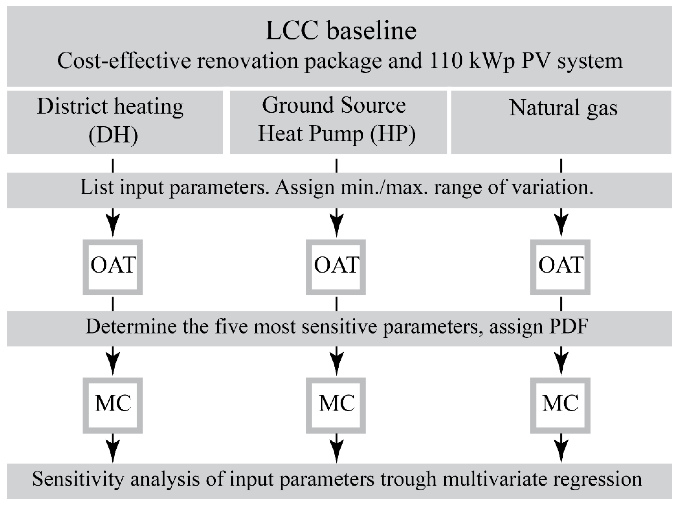
2. Method
2.1. Life Cycle Cost Calculation Method
- COINIT—initial cost;
- COa—annual cost;
- COCO2—emission cost;
- COfin(TSL)—disposal cost;
- VALft—residual value;
- D_f—discount factor;
- tTC—calculation period;
- RATxx(i) price evolution of parameter i.
2.1.1. Model Boundary Conditions
- Decreasing real DR—This DR type is applied to public buildings where a 1% decrease is applied after years 36 and 75. This DR type applies fixed prices without inflation [32].
- Fixed real DR—Applied to projects concerning social housing organizations. As the name suggests, the DR and possible PD are fixed and exclude inflation.
- Fixed Nominal DR—Prices and DR are stated in current prices, including inflation. This DR type is applied to projects requiring DGNB certification.
2.1.2. Model Inputs
2.2. Local Sensitivity Analysis—OAT
- District heating (DH)—the unit price for district heating is available for 392 DH plants across Denmark. There is great variation in the cost of delivered heat across Denmark. Therefore, cost data in [38] are given as annual values for 2018—found in the 392 different DH plants and not as historical values—for electricity and gas. The average price for 2018 from the different stations is 525 DKK/MWh and varies significantly from one DH plant to the next (±135 DKK/kWh). The range for OAT calculations is determined by the minimum and maximum value, accessible in the database.
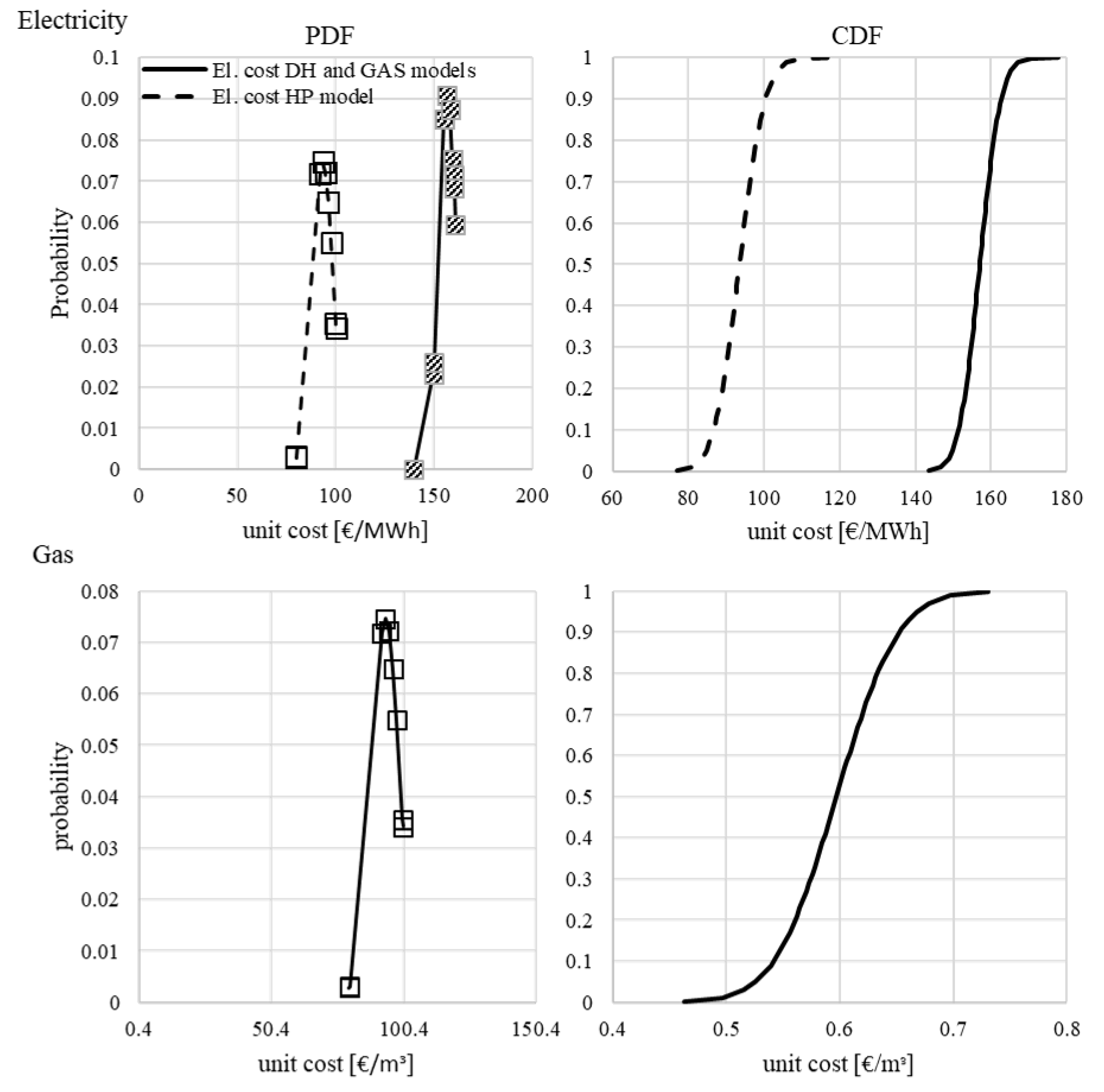
- Electricity—the unit cost of electricity is a quite complex and uncertain parameter. The final unit cost depends on the “raw” energy price and several other factors influencing the price. Some of the main factors are governmental fees and taxes, provider subscription expenses, network maintenance, and fees. Moreover, some of those fees are fixed while others are added concerning the building heating system and demand. For example, a general charge of 88.4 øre/kWh is added to the electricity price. If the building is heated by electricity, an additional 25.9 øre/kWh is owed by each client (building owner) [38]. Moreover, a variable “PSO (Public service obligation)” is added when forming the final electricity price. As all of those price elements are highly variable and continuously evolving, they are thereby excluded from the calculations along with VAT, taxes, and fees. In addition to all taxes and fees, electricity price is also dependent on the annual amount of purchased electricity by the “client” of the energy providers, e.g., apartment tenants or building owners. Clients of a supply company are classified into categories (usage intervals) from small (single-family homes) to large (industrial clients). Naturally, the unit cost for large clients is lower than that for small clients. As the baseline considers a multi-family building, the baseline value was selected considering medium-size client (usage interval from 2.5 < 5 MWh) and determined as the average of available annual cost data for 2009–2018 [33]. It should be pointed out that the analysis presented in [28] and those presented in this paper account for the purchase of electricity for the whole building globally (e.g., building operation and private use in apartments are analyzed as inputs). In reality, the building owner and each tenant would be individual clients of the electricity provider. Thus, tenants would be categorized/charged according to costs with respect to low usage intervals, while the building owner would likely be categorized as a client in the higher usage intervals with lower unit costs. The range applied in OAT analysis represents the minimum and maximum annual values for electricity costs of different usage intervals to investigate the effect of this simplification.
- Gas—unit costs for gas are also differentiated by client type (household or industry) and by the amount of purchased energy. A breakdown of household gas prices is provided monthly for the period from 2009–2018. Each aspect contributing to the total gas price is represented individually. Given that the gas price has been rather stable [33] for the period from 2009–2018, the baseline value was determined by average cost, while the OAT range was determined as the minimum and maximum values for the whole period and excluding VAT. Gas prices are also available as annual values for different usage intervals (client sizes). In a scenario where gas is the source for centralized heating and DHW supply, the energy demand of the building would be a determining factor for the unit cost of gas. However, just as for electricity, governmental taxes and local subscription tariffs are also major determining factors for the total cost. Those are included in the OAT variation, as the baseline adapts average, minimum, and maximum values from 2007–2018, excluding VAT but including government taxes and levies. Furthermore, baseline values were selected based on the smallest available usage interval (<20 GJ gas).
2.3. Global Sensitivity—Monte Carlo (MC) Method
2.4. Sensitivity Analysis
3. Results
3.1. Local Sensitivity—One-at-a-Time (OAT) Approach
3.1.1. Boundary Conditions
3.1.2. Model Inputs
3.2. Global Sensitivity
3.2.1. Variated Parameters
3.2.2. Sensitivity Analysis
3.3. Global Cost Robustness of the Baseline
4. Discussion
5. Conclusions
- This study examined the relationship between the input and output of LCC calculations for a pre-selected renovation case of a residential building in Denmark.
- The study sheds light on the currently available data and sources for the inputs required for LCC calculations, focused on renovation expenditures.
- The applied approach consists of one-at-a-time (OAT) and Monte Carlo (MC) methods for the variation of the inputs. A simple first-order sensitivity index was calculated for all the model inputs variated with the OAT method to compare the sensitivity of the parameters and select the most influential ones for further variation with the MC method. The investigation of the interactive effects of the variated parameters on the output was quantified using linear regression and the analysis of the standardized regression coefficients for the selected parameters.
- Performing OAT variation on the boundary conditions and building-related inputs enabled the comparison of the individual effects of the three boundary conditions: the discount rate (DR) type, price development (PD), and calculation period. Based on the results, it can be concluded that the DR type and PD for electricity and district heat have approximately the same effect. At the same time, the variation in the calculation period showed greater sensitivity indexes for the studied scenarios. However, these results should be taken with caution, as they represent the individual effect of each input on the output and not the interactive effects of all inputs.
- The OAT method’s results implied a linear relationship between the input and outputs, which was verified by the high R2 values resulting from a regression analysis of the MC results for all studied models. Furthermore, the applied regression method (Sensitivity-Ranked Regression Coefficients) ranked each of the five variated parameters with respect to the output’s sensitivity to each one.
- The financial parameters and calculation period in Denmark can be considered deterministic, as their values are determined by legislation.
- Given that specific values are determined concerning the investigated building type, the variation applied in this paper is aimed at quantifying the expected variance when a different set of boundary condition assumptions is used in the selected baseline. The applied OAT approach to building-related model inputs showed that energy demand-related inputs are the most influential.
- The global sensitivity analysis shows that the calculation models with District Heating (DH) and gas reveal that the most influential inputs are about twice as sensitive as the next most influential ones. In those cases, the relative importance of the parameters of DH and gas is nearly equal, with a slight variation between the ranking in the two cases. On the contrary, for a scenario with a Heat Pump (HP), the lifetime of the HP is determined as the most sensitive. Moreover, the relative difference in the regression coefficient values (importance) for the different parameters in the HP case is much smaller than the DH and gas cases.
- This study adds to the understanding of the relationship between the inputs and output for LCC calculations, considering a cost-effective renovation package combined with three energy supply systems for heating and DHW production.
Author Contributions
Funding
Institutional Review Board Statement
Informed Consent Statement
Conflicts of Interest
Nomenclature
| NZEB | Nearly Zero Energy Building |
| EU | European Union |
| LCC | Life Cycle Cost |
| OAT | One-at-a-time |
| MC | Monte Carlo |
| HP | Heat Pump |
| DHW | Domestic Hot Water |
| DH | District Heating |
| PV | Photovoltaic |
| GC | Global Cost |
| NPV | Net Present Value |
| DR | Discount Rate |
| PD | Price Development |
| TDC | Technology Data Catalogue |
| DEA | Danish Energy Agency |
| IR | Interest Rate |
| SA | Sensitivity Analysis |
| SRRC | Standardized Rank Regression Coefficient |
| SI | Sensitivity Index |
| Probability Density Function | |
| CDF | Cumulative Distribution Function |
| CO | Cost type |
| Difference between the output values obtained from the minimum and maximum variated input value of parameter i | |
| bi | Regression coefficient |
| Standard deviation | |
| µ | Mean |
| COINIT | Initial cost |
| COa | Annual cost |
| COCO2 | Emission cost |
| COfin(TSL) | Disposal cost |
| VALe5 | Residual value |
| D_f | Discount factor |
| tTC | Calculation period. |
| RAT | (i) price evolution of parameter i- |
Appendix A


| Parameter xi | New Windows | Attic Insulation | Roof-Mounted PV | Attic Insulation | Electricity | ε |
|---|---|---|---|---|---|---|
| Attribute | unit price | Amount | Unit price | Unit price | Unit price | |
| Coefficients | −0.82258 | −0.393233267 | −0.27311281 | −0.29911744 | −0.04455671 | −4.15 × 10⁻¹⁶ |
| Standard error values of coefficients | 0.000643 | 0.000642742 | 0.000642742 | 0.000642742 | 0.000642742 | 0.000642741 |
| R2 | 0.997937 | 0.045448669 | #N/A | #N/A | #N/A | #N/A |
| Regression—sum of squares | 483,126.4 | 4994 | #N/A | #N/A | #N/A | #N/A |
| Residual sum of squares | 4989.684 | 10.31551425 | #N/A | #N/A | #N/A | #N/A |

| Parameter xi | Gas | Attic Insulation | Roof-Mounted PV | Attic Insulation | Electricity | ε |
|---|---|---|---|---|---|---|
| Attribute | unit price | Amount | Unit price | Unit price | Unit price | |
| Coefficients | −1.2292 | −0.587637 | −0.408132 | −0.44699 | −0.06658 | 5.561 |
| Standard error values of coefficients | 0.00096 | 0.000960 | 0.000960 | 0.000960 | 0.000960 | 0.00096 |
| R2 | 0.997937 | 0.067917 | #N/A | #N/A | #N/A | #N/A |
| Regression—sum of squares | 483,126.4 | 4994 | #N/A | #N/A | #N/A | #N/A |
| Residual sum of squares | 11142.74 | 23.0361 | #N/A | #N/A | #N/A | #N/A |

| Parameter xi | Heat Pump | Attic Insulation | Roof-Mounted PV | Attic Insulation | Electricity | ε |
|---|---|---|---|---|---|---|
| Attribute | Lifetime | Amount | Unit price | Unit price | Unit price | |
| Coefficients | 0.57032 | −0.525506908 | −0.365908376 | −0.39981676 | −0.30338984 | −1.12 × 10⁻¹⁴ |
| Standard error values of coefficients | 0.001635 | 0.001634858 | 0.001634856 | 0.001634856 | 0.001634857 | 0.00163 |
| R2 | 0.986652 | 0.115601688 | #N/A | #N/A | #N/A | #N/A |
| Regression—sum of squares | 73,830.49 | 4994 | #N/A | #N/A | #N/A | #N/A |
| Residual sum of squares | 4933.261 | 66.73856858 | #N/A | #N/A | #N/A | #N/A |
References
- European Commission. Directive (EU) 2018/2002 of the European Parliament and of the Council of 11 December 2018 Amending Directive 2012/27/EU on energy efficiency. Off. J. Eur. Union 2018, 328, 210–230. [Google Scholar]
- European Union. Directive (EU) 2018/844 of the European Parliament and of the Council of 30 May 2018 amending Directive 2010/31/EU on the energy performance of buildings and Directive 2012/27/EU on energy efficiency. Off. J. Eur. Union 2018, 156, 75–91. [Google Scholar]
- Bolig og Planstyrrelsen. Available online: https://baeredygtighedsklasse.dk/ (accessed on 10 September 2022).
- Ministry of the Interior and Housing. Available online: https://im.dk/Media/637602217765946554/National_Strategy_for_Sustainable_Construktion.pdf (accessed on 10 September 2022).
- Ferreira, M.; Almeida, M.; Rodrigues, A. Cost-optimal energy efficiency levels are the first step in achieving cost-effective renovation in residential buildings with a nearly-zero energy target. Energy Build. 2016, 133, 724–737. [Google Scholar] [CrossRef]
- Congedo, P.M.; D’Agostino, D.; Baglivo, C.; Tornese, G.; Zacà, I. Efficient Solutions and Cost-Optimal Analysis for Existing School Buildings. Energies 2016, 9, 851. [Google Scholar] [CrossRef]
- Morrissey, J.; Horne, R. Life cycle cost implications of energy efficiency measures in new residential buildings. Energy Build. 2011, 43, 915–924. [Google Scholar] [CrossRef]
- Sağlam, N.G.; Yılmaz, A.Z.; Becchio, C.; Corgnati, S.P. A comprehensive cost-optimal approach for energy retrofit of existing multi-family buildings: Application to apartment blocks in Turkey. Energy Build. 2017, 150, 224–238. [Google Scholar] [CrossRef]
- DS/EN 15459-1:2017; Energy Performance of Buildings—Economic Evaluation Procedure for Energy Systems in Buildings—Part 1: Calculation Procedured, Module M1—14. European Committee for Standartization: Brussels, Belgium, 2017.
- Giuseppe, E.D.; Massi, A.; D’Orazio, M. Impacts of Uncertainties in Life Cycle Cost Analysis of Buildings Energy Efficiency Measures: Application to a Case Study. Energy Procedia 2017, 111, 442–451. [Google Scholar] [CrossRef]
- Burhenne, S.; Tsvetkova, O.; Jacob, D.; Henze, G.P.; Wagner, A. Uncertainty quantification for combined building performance and cost-benefit analyses. Build. Environ. 2013, 62, 143–154. [Google Scholar] [CrossRef]
- Janssen, H. Monte-Carlo based uncertainty analysis: Sampling efficiency and sampling convergence. Reliab. Eng. Syst. Saf. 2013, 109, 123–132. [Google Scholar] [CrossRef]
- Heiselberg, P.; Brohus, H.; Hesselholt, A.; Rasmussen, H.; Seinre, E.; Thomas, S. Application of sensitivity analysis in design of sustainable buildings. Renew. Energy 2009, 34, 2030–2036. [Google Scholar] [CrossRef]
- Wei, T. A review of sensitivity analysis methods in building energy analysis. Renew. Sustain. Energy Rev. 2013, 20, 411–419. [Google Scholar] [CrossRef]
- Østergård, T.; Jensen, R.L.; Maagaard, S.E. Early Building Design: Informed decision-making by exploring multidimensional design space using sensitivity analysis. Energy Build. 2017, 142, 8–22. [Google Scholar] [CrossRef]
- Østergård, T.; Jensen, R.L.; Mikkelsen, F.S. The best way to perform building simulations? One-at-a-time optimization vs. Monte Carlo sampling. Energy Build. 2020, 208, 109628. [Google Scholar] [CrossRef]
- Ruparathna, R.; Hewage, K.; Sadiq, R. Economic evaluation of building energy retrofits: A fuzzy based approach. Energy Build. 2017, 139, 395–406. [Google Scholar] [CrossRef]
- La Fleur, L.; Rohdin, P.; Moshfegh, B. Investigating cost-optimal energy renovation strategies for a multifamily building in Sweden. Energy Build. 2019, 203, 109438. [Google Scholar] [CrossRef]
- Guardigli, L.; Bragadin, M.A.; Della Fornace, F.; Mazzoli, C.; Prati, D. Energy retrofit alternatives and cost-optimal analysis for large public housing stocks. Energy Build. 2018, 166, 48–59. [Google Scholar] [CrossRef]
- Pallis, P.; Gkonis, N.; Varvagiannis, E.; Braimakis, K.; Karellas, S.; Katsaros, M.; Vourliotis, P.; Sarafianos, D. Towards ΝZEB in Greece: A comparative study between cost optimality and energy efficiency for newly constructed residential buildings. Energy Build. 2019, 198, 115–137. [Google Scholar] [CrossRef]
- Pallis, P.; Gkonis, N.; Varvagiannis, E.; Braimakis, K.; Karellas, S.; Katsaros, M.; Vourliotis, P. Cost effectiveness assessment and beyond: A study on energy efficiency interventions in Greek residential building stock. Energy Build. 2019, 182, 1–18. [Google Scholar] [CrossRef]
- Liu, L.; Rohdin, P.; Moshfegh, B. LCC assessments and environmental impacts on the energy renovation of a multi-family building from the 1890s. Energy Build. 2016, 133, 823–833. [Google Scholar] [CrossRef]
- Sandberg, N.H.; Sartori, I.; Vestrum, M.I.; Brattebø, H. Using a segmented dynamic dwelling stock model for scenario analysis of future energy demand: The dwelling stock of Norway 2016–2050. Energy Build. 2017, 146, 220–232. [Google Scholar] [CrossRef]
- Hamdy, M.; Sirén, K.; Attia, S. Impact of financial assumptions on the cost optimality towards nearly zero energy buildings—A case study. Energy Build. 2017, 153, 421–438. [Google Scholar] [CrossRef]
- Ascione, F.; Bianco, N.; De Stasio, C.; Mauro, G.M.; Vanoli, G.P. CASA, cost-optimal analysis by multi-objective optimisation and artificial neural networks: A new framework for the robust assessment of cost-optimal energy retrofit, feasible for any building. Energy Build. 2017, 146, 200–219. [Google Scholar] [CrossRef]
- Gonzalez-Caceres, A.; Karlshøj, J.; Vik, T.A.; Hempel, E.; Nielsen, T.R. Evaluation of cost-effective measures for the renovation of existing dwellings in the framework of the energy certification system: A case study in Norway. Energy Build. 2022, 264, 112071. [Google Scholar] [CrossRef]
- Di Giuseppe, E.; Iannaccone, M.; Telloni, M.; D’Orazio, M.; Di Perna, C. Probabilistic life cycle costing of existing buildings retrofit interventions towards nZE target: Methodology and application example. Energy Build. 2017, 144, 416–432. [Google Scholar] [CrossRef]
- Antonov, Y.I.; Heiselberg, P.K.; Pomianowski, M.Z. Novel Methodology toward Nearly Zero Energy Building (NZEB) Renovation: Cost-Effective Balance Approach as a Pre-Step to Cost-Optimal Life Cycle Cost Assessment. Appl. Sci. 2021, 11, 4141. [Google Scholar] [CrossRef]
- Antonov, Y.I.; Heiselberg, P.; Flourentzou, F.; Pomianowski, M.Z. Methodology for Evaluation and Development of Refurbishment Scenarios for Multi-Story Apartment Buildings, Applied to Two Buildings in Denmark and Switzerland. Buildings 2020, 10, 102. [Google Scholar] [CrossRef]
- Aalborg University. LCCbyg; Aalborg University: Copenhagen, Denmark, 2020. [Google Scholar]
- Danish Ministry of Finance. Den Samfundsøkonomiske Diskonteringsrente; Finance Minister: Copenhagen, Denmark, 2019. [Google Scholar]
- Danish Ministry of Finance. Dokumentationsnotat—Den Samfundsøkonomiske Diskonteringsrente; Danish Ministry of Finance: Cophenhagen, Denmark, 2021; pp. 1–19. [Google Scholar]
- Energistyrelsens Prisdatabase 2019; Danish Energy Agency: Copenhagen, Denmark, 2019.
- Danish Energy Agency and Energinet. Technology Data for Individual Heating Plants; Danish Energy Agency and Energinet: Copenhagen, Denmark, 2016. [Google Scholar]
- Danish Energy Agency. Technology Data for Energy Plants for Electricity and District Heating Generation; Danish Energy Agency: Copenhagen, Denmark, 2019; pp. 1–374. [Google Scholar]
- MOLIO Price Database. Available online: https://www.molio.dk/emner/oekonomi-og-kalkulation/prisdata (accessed on 10 September 2022).
- Aagaard, N.-J.; Brandt, E.; Aggerholm, S.; Haugbølle, K. Levetider af Bygningsdele ved Vurdering af Bæredygtighed og Totaløkonomi; SBI Forlag: Copenhagen, Denmark, 2013; ISBN 978-87-563-1586-9. [Google Scholar]
- Elforsyningens Nettariffer & Priser pr. 1. Januar 2019; Dansk Energi: Viby, Denmark, 2019.
- Samfundsøkonomiske Beregningsforudsætninger for Energipriser Og Emissioner, Oktober 2019; Danish Energy Agency: København, Denmark, 2019.


| Baseline | OAT | |||||
|---|---|---|---|---|---|---|
| Category | Parameter | Unit | Value | Source | Range | Source |
| Operation | * District heating | EUR/MWh | 69.29 | DEA [33] | 18–128 | Database min/max |
| (Energy supply) | * Gas | EUR/m3 | 0.796 | 0.635–0.913 | ||
| * Electricity | EUR/MWh | 230.1 | 210–330 | |||
| * Electricity-HP | EUR/MWh | 93.54 | - | |||
| Implementation | * DH sub-station | EUR/system | 15,600 | TDC [34] | 12–20 K | TDC [25] |
| * Gas boiler | EUR/unit | 24,600 | 20–30 K | |||
| * Heat Pump | EUR/unit | 249,000 | 235–265 K | |||
| Roof-mounted PV | EUR/system | 80,300 | TDC [35] | 49.5–134.2 K | Assumed ±20% | |
| Ex. wall insulation | EUR/m2 | 20.7 | MOLIO [36] | 17–25 | Assumed ±20% | |
| Ex. wall cladding | EUR/m2 | 17 | 13–20 | |||
| New windows | EUR/m2 | 73 | 69–88 | |||
| Attic insulation | EUR/m2 | 130 | 104–156 | |||
| Pipe network ins. | EUR/m | 11.8 | 9–14 | |||
| Circulation pump | EUR/unit | 1098 | 879–1318 | |||
| Maintenance | * DH sub-station | EUR/year | 136 | TDC [34] | 108–189 | TDC [25] |
| * Gas boiler | EUR/year | 651 | 531–814 | |||
| * Heat Pump | EUR/year | 1650 | 1070–2850 | |||
| Roof-mounted PV | EUR/year | 1144 | TDC [35] | 781–1342 | TDC [26] | |
| Ex. wall insulation | EUR/year | 551 | LCCByg* | 440–660 | Assumed ±20% | |
| Ex. wall cladding | EUR/year | 894 | 715–1072 | |||
| Windows | EUR/year | 1147 | 918–1376 | |||
| Attic insulation | EUR/year | 228 | 1814–2722 | |||
| Pipe network ins. | EUR/year | 373 | 298–447 | |||
| Circulation pump | EUR/year | 11 | 9–13 | |||
| Lifespan | * DH sub-station | year | 25 | TDC [34] | 20–30 | TDC [25] |
| * Gas boiler | year | 25 | 25–40 | |||
| * Heat Pump | year | 20 | 15–25 | |||
| Roof-mounted PV | year | 30 | TDC [35] | 25–40 | TDC [26] | |
| Ex. wall insulation | year | 50 | sbi [37] | 40–60 | Assumed ±20% | |
| Ex. wall cladding | year | 120 | 95–145 | |||
| Windows | year | 50 | 40–60 | |||
| Attic insulation | year | 50 | 35–65 | |||
| Pipe network ins. | year | 80 | 65–95 | |||
| Circulation pump | year | 25 | 20–30 | |||
| Amount | * District heating | MWh | 483.37 | calculated BE18 | 387–580 | Assumed ±20% |
| * Gas | m3 | CC | ||||
| * Electricity—DH and gas | MWh | 51,072 | 41.6–62.4 K | |||
| * Electricity—HP | MWh | 216.8 | ||||
| Ex. wall insulation | m2 | 2660 | Measured | 2128–3192 | Assumed ±20% | |
| Ex. wall cladding | m2 | 2660 | 2128–3192 | |||
| Windows | m2 | 1570 | 1256–1885 | |||
| Attic insulation | m2 | 1750 | 1400–2100 | |||
| Pipe network ins. | m2 | 3160 | 2528–3792 | |||
| Rank according to Sensitivity Index | |||||
|---|---|---|---|---|---|
| 1 | 2 | 3 | 4 | 5 | |
| District heating | unit cost electricity | unit cost attic insulation | unit cost roof PV | amount attic insulation | unit cost new windows |
| Heat pump | lifetime heat pump | unit cost electricity | unit cost attic insulation | amount attic insulation | unit cost roof PV |
| Gas | unit cost natural gas | unit cost electricity | unit cost attic insulation | amount attic insulation | unit cost roof PV |
| Category | Parameter | Unit | Probability Density Function | Source | |
|---|---|---|---|---|---|
| Operation | Electricity—DH and gas | EUR/MWh | Normal | µ = 157; σ = 4.39 | DEA [37,39] |
| Electricity—HP | EUR/MWh | Normal | µ = 93.5; σ = 5.35 | DEA [37,39] | |
| gas | EUR/m3 | Normal | µ = 0.6; σ = 0.04 | DEA [37,39] | |
| Implementation | Attic insulations | EUR/m2 | Uniform | 104–156 | Assumed |
| Roof-mounted PV | EUR/system | Uniform | 49.5–134.2 K | TDC [35] | |
| New windows | EUR/m2 | Normal | µ = 147.1; σ = 50 | Assumed | |
| Lifespan | Heat pump | year | Uniform | 15–25 | TDC [34] |
| Amount | Attic insulation | m2 | Uniform | 1400–2400 | Assumed |
| Nr. | Variable | Sensitivity | Standardised Regression Coefficient (SRC) | ||
|---|---|---|---|---|---|
 | DH | GAS | HP | ||
| 1 | Electricity unit cost |  | −0.029 | ||
| −0.067 | |||||
| −0.303 | |||||
| 2 | Attic insulation unit cost |  | −0.299 | ||
| −0.447 | |||||
| −0.400 | |||||
| 3 | PV unit cost |  | −0.237 | ||
| −0.408 | |||||
| −0.366 | |||||
| 4 | Attic insulation amount |  | −0.393 | ||
| −0.588 | |||||
| −0.526 | |||||
| 5 | Model DH: New windows unit cost |  | −0.823 | ||
| 6 | Model: Gas Gas unit cost |  | −1.229 | ||
| 7 | Model Gas: Lifetime of HP |  | 0.57 | ||
 | |||||
Publisher’s Note: MDPI stays neutral with regard to jurisdictional claims in published maps and institutional affiliations. |
© 2022 by the authors. Licensee MDPI, Basel, Switzerland. This article is an open access article distributed under the terms and conditions of the Creative Commons Attribution (CC BY) license (https://creativecommons.org/licenses/by/4.0/).
Share and Cite
Antonov, Y.I.; Jønsson, K.T.; Heiselberg, P.; Pomianowski, M.Z. Investigations of Building-Related LCC Sensitivity of a Cost-Effective Renovation Package by One-at-a-Time and Monte Carlo Parameter Variation Methods. Appl. Sci. 2022, 12, 9817. https://doi.org/10.3390/app12199817
Antonov YI, Jønsson KT, Heiselberg P, Pomianowski MZ. Investigations of Building-Related LCC Sensitivity of a Cost-Effective Renovation Package by One-at-a-Time and Monte Carlo Parameter Variation Methods. Applied Sciences. 2022; 12(19):9817. https://doi.org/10.3390/app12199817
Chicago/Turabian StyleAntonov, Yovko Ivanov, Kim Trangbæk Jønsson, Per Heiselberg, and Michal Zbigniew Pomianowski. 2022. "Investigations of Building-Related LCC Sensitivity of a Cost-Effective Renovation Package by One-at-a-Time and Monte Carlo Parameter Variation Methods" Applied Sciences 12, no. 19: 9817. https://doi.org/10.3390/app12199817
APA StyleAntonov, Y. I., Jønsson, K. T., Heiselberg, P., & Pomianowski, M. Z. (2022). Investigations of Building-Related LCC Sensitivity of a Cost-Effective Renovation Package by One-at-a-Time and Monte Carlo Parameter Variation Methods. Applied Sciences, 12(19), 9817. https://doi.org/10.3390/app12199817