Article

Comparison of Canopy Cover and Leaf Area Index Estimation from Airborne LiDAR and Digital Aerial Photogrammetry in Tropical Forests

1
Industry Development and Planning Institute, National Forestry and Grassland Administration, Beijing 100010, China
2
Academy of Inventory and Planning, National Forestry and Grassland Administration, Beijing 100714, China
3
Research Center of Forest Management Engineering of State Forestry and Grassland Administration, Beijing Forestry University, Beijing 100083, China
*
Author to whom correspondence should be addressed.
These authors contributed to the work equally and should be regarded as co-first authors.
Appl. Sci. 2022, 12(19), 9882; https://doi.org/10.3390/app12199882
Submission received: 11 August 2022 / Revised: 8 September 2022 / Accepted: 23 September 2022 / Published: 30 September 2022
(This article belongs to the Special Issue Advances in Geospatial Techniques on Ecosystem Monitoring)

Abstract

:
Digital aerial photogrammetry (DAP) has emerged as an alternative to airborne laser scanning (ALS) for forest inventory applications, as it offers a low-cost and flexible three-dimensional (3D) point cloud. Unlike the forest inventory attributes (e.g., tree height and diameter at breast height), the relative ability of DAP and ALS in predicting canopy structural variables (i.e., canopy cover and leaf area index (LAI)) has not been sufficiently investigated by previous studies. In this study, we comprehensively compared the canopy cover and LAI estimates using DAP- and ALS-based methods over 166 selected tropical forest sample plots with seven different tree species and forest types. We also explored the relationship between field-measured aboveground biomass (AGB) and the LAI estimates. The airborne LAI estimates were subsequently compared with the Sentinel-2-based LAI values that were retrieved using a one-dimensional radiative transfer model. The results demonstrated that the DAP-based method generally overestimated the two canopy variables compared to ALS-based methods but with relatively high correlations regardless of forest type and species (R2 of 0.80 for canopy cover and R2 of 0.76 for LAI). Under different forest types and species, the R2 of canopy cover and LAI range from 0.64 to 0.89 and from 0.54 to 0.87, respectively. Apparently, different correlations between AGB and LAI were found for different forest types and species where the mixed coniferous and broad-leaved forest shows the best correlation with R2 larger than 0.70 for both methods. The comparison with satellite retrievals verified that the ALS-based estimates are more consistent with Sentinel-2-based estimates than DAP-based estimates. We concluded that DAP data failed to provide analogous results to ALS data for canopy variable estimation in tropical forests.

1. Introduction

Canopy structure is characterized by the position, orientation, size, and shape of the vegetative elements [1]. Canopy cover and leaf area index (LAI) are two canopy structural variables that are critical for many forest and ecological applications [2,3,4,5]. They are commonly used as ecological indicators [6] and input parameters for biosphere modeling [7]. Both of them play a vital role in ecological and physical processes, such as photosynthesis, transpiration, and carbon cycling [8]. Canopy cover was defined as the proportion of the forest floor covered by the vertical projection of the tree crowns [4] and was then extended to the area of the vertical projection of the outermost perimeter of the crown on the horizontal plane [2]. LAI was first defined as the total one-sided area of photosynthetic tissue per unit of ground surface area for broad-leaf forests [9] and consequently LAI was defined as the maximum projected leaf area per unit of ground surface area [10]. Multispectral remote sensing has been widely used to estimate these parameters through statistical methods based on field measurements [11] or physical methods based on a radiative transfer model [12]. However, those approaches cannot obtain direct indications of canopy structure, in both horizontal and vertical dimensions [13]. Therefore, methods which can provide canopy structural information in three-dimensional (3D) space with high precision can improve the estimation of canopy cover and LAI [14,15,16].
During the past 20 years, airborne laser scanning (ALS) systems have become primary data collectors for 3D characteristics of canopy and forest structure [13]. Therefore, ALS systems are proven to be efficient tools to estimate forest 3D structure parameters from 3D point clouds [15,17]. Different methods have been applied to estimate canopy cover and LAI from ALS data. Regression methods use different variable metrics based on ALS data and ground measurements to quantify the complexity of forest canopies [18]. Contact frequency methods are based on the contact frequency, and calculate the probability of a beam penetrating the canopy coming into contact with a vegetative element [19]. The accuracy of contact frequency methods depends on the size of voxels and they are time-consuming during data acquisition and registration processes [20]. Gap fraction methods generate the correlation between LAS data and an area property such as gap fraction and canopy cover, where the return of each pulse is classified as either canopy or gap [21]. Based on the Beer–Lambert law, canopy cover can be further converted into LAI by inverting the gap fraction and log-transformation [22]. Studies have demonstrated that such log-transformed, inverted gap fraction data from ALS are in good agreement with field measurements [16,23,24].
With the recent development of small aircraft technology over recent years, aerial photographs from digital cameras have been widely used in forest inventory. Compared with ALS systems, they are more cost-efficient and suitable for continuous monitoring over large areas with good availability [25,26]. Point clouds are generated from the digital images through the structure from motion (SfM) algorithm [27], which is one of the digital aerial photogrammetry (DAP) techniques. For single-layered forests, forest attributes such as canopy height model (CHM) and LAI can be captured well from DAP and show good agreement with ALS-based results [15,28]. For more complex forest environments, even though there are difficulties for DAP to estimate under-canopy structural and terrain information, accurate upper canopy structure can be obtained with the input digital terrain models (DTMs) [29,30]. Therefore, more efforts are still needed to explore the potentiality of DAP to estimate canopy structural variables for forestry applications.
This study aimed to compare the performance of airborne LiDAR and digital imagery in the estimation of canopy cover and LAI in tropical forests. Airborne LiDAR and digital imagery were first processed. Methods to estimate canopy cover and LAI from two data sources were then presented. The estimated results from both airborne LiDAR and digital imagery were compared together with the results from Sentinel-2 data and the relationship between canopy cover, LAI, and tree height were investigated. Finally, we discuss the implications of our results for further forestry inventory.

2. Materials

2.1. Study Area and Field Inventory of Plots

The study area is located in a national tropical rainforest park in Hainan Province, China (108°36′~109°57′ E, 18°23′~19°11′ N), covering approximately 4900 km2 with elevation ranging from 100 m to 1876 m (Figure 1). The region is characterized by a tropical maritime monsoon climate with annual average temperature of 22.5~26.0 °C and annual average precipitation of 1759 mm. Mixed broad-leaved forests and pure broad-leaved forests are the main land cover types in the study area where rubber tree (Hevea spp.), eucalyptus (Eucalyptus spp.), and Taiwan acacia (Acacia spp.) are dominant among various tree species. To evaluate the relationship between remotely sensed estimated canopy structural variables (i.e., canopy cover and LAI) and forest inventory variables (i.e., tree height, diameter at breast height (DBH), crown diameter), we conducted a field campaign to measure the forest inventory variables. Three canopy coverage levels and five tree height levels were set in the selection of forest sample plots, resulting in 166 plots with a diameter of 30 m. These plots were positioned according to the trade-off between the accessibility and the random sampling rule.
We used a real-time kinematic (RTK) GPS to accurately measure the plot center and each tree’s position in every forest plot. The age group of each plot was recorded where the tree age was measured by counting the tree rings obtained by a growth cone. The dominant tree species in each mixed forest plot was also recorded where the dominant species was identified according to the ratio of the number of a specific tree species to the total. Tree height and DBH of each tree were separately measured by a laser altimeter (Haglof Vertex Laser developed by Haglöf Sweden) and a tape measure. The crown diameter was estimated by averaging two measurements taken from two measuring tapes laid perpendicular to each other at the largest width of each crown. These plots were categorized into seven types according to the forest species which include 6 mixed coniferous and broad-leaved forest plots, 18 mixed broad-leaved forest plots, 49 Eucalyptus robusta Smith plots, 30 Acacia confusa Merr. plots, 49 Hevea brasiliensis plots, 2 Chinese fir plots, and 12 other coniferous trees plots. The AGBs of all tree species and forest types were calculated using allometry equations (Table 1) [31].

2.2. Airborne LiDAR Data and Preprocess

We conducted aerial campaigns over the study area from March 2020 to February 2021 using the National Forest and Grassland Inventory Airborne Observatory Platform that is an integrated observation equipment with a small-footprint LiDAR (RIEGL VQ-1560i (Riegl GmbH, Horn, Austria) with a laser wavelength of 1064 nm), a digital imager (Phase One iXU-RS 1000 (Phase One Inc, Copenhagen, Denmark)), and a position and orientation system (Applanix AP-60 (Trimble Inc., Sunnyvale, CA, USA)). The LiDAR uses an analogue detector to record discrete, time-stamped trigger pulses from the received waveform in real time, i.e., the discrete-return system. The airplane (Cessna 208B-9617) flew at a relative flight altitude of about 1800 m relative to the take-off point and with flight speed of around 260 km/h, resulting in a LiDAR beam diameter of about 0.45 m. The laser emission frequency is 2000 kHz and the lateral overlap of LiDAR was set as 22%.
After airborne LiDAR (ALS) data acquisition, the aircraft GPS trajectories for each airborne survey were firstly corrected to the ground-based GPS base station using the POSpac version 8. 3 software (Trimble Inc., Sunnyvale, CA, USA). The scan angles and laser pulse return were then integrated with the trajectories using the RiProcess version 1.8.5 software (Riegl GmbH, Horn, Austria). The point cloud files were finally exported and geographic coordinates, elevation, and intensity information were included. Based on 263 ground control points, the horizontal and vertical errors were less than 0.15 m and 0.08 m, respectively.
The ALS point clouds were classified into ground return and other returns using the cloth simulation filter (CSF) algorithm [32]. The digital terrain model (DTM) with spatial resolution of 1 m was created using the ground points with the k-nearest neighbor with inverse distance weighting interpolation algorithm. The produced ALS-based DTM (DTMALS) was used to normalize the ALS point clouds and subsequently used in the process of airborne image-based point clouds. After normalization, all elevations of points were relative to the same ground level datum. The ALS point clouds were divided into canopy returns and below-canopy returns using a height threshold of 2.0 m.

2.3. Airborne Digital Imagery and Preprocess

The airborne digital imager was equipped with a 50 mm focal length lens and a 11,608 × 8708-pixel (4.6 μm physical pixel size) sensor, resulting in a field of view of 56.2° × 43.7°. The imager achieved a ground resolution of 0.165 m relative to the flight altitude of 1800 m. The forward overlap and side overlap of the imager are 63% and 20%, respectively.
After airborne digital imagery acquisition, the position information and orientation information of each image were extracted based on the onboard GPS and IMU data. The red–green–blue (RGB) images were processed by a photogrammetry technique, so-called digital aerial photogrammetry (DAP). The overlapped RGB images with the corresponding geographic coordinates of waypoints were imported into Agisoft Metashape Pro (Agisoft LLC, St. Petersburg, Russia) to produce a dense point cloud and a georeferenced DSM. Our processing steps are identical to the recommended photogrammetry processing pipeline, as can be found in the Metashape user manual. The resulting point density of DAP was around 50 points/m2 while, in contrast, the point density of ALS was about 10 points/m2.
The DAP and LiDAR point clouds of the entire study area were firstly co-registered through a coarse adjustment by hand then a fine iterative closest point (ICP) algorithm. After the co-registration, the DAP and LiDAR point clouds were processed according to the boundary of forest plots. For each plot, the co-registration between DAP and LiDAR point clouds was fine-tuned using the ICP algorithm to achieve the optimal co-registration in local extent. The point clouds of each plot were denoised to remove isolated outlier points using a manual trimming by visual interpretation and automatic noise removal by a median filter in CloudCompare version 2.11.0 software (https://www.danielgm.net/cc/, accessed on 10 August 2022). The DAP-based digital surface model (DSMDAP) with grid size (i.e., spatial resolution) of 1 m was then created using all points with the k-nearest neighbor with inverse distance weighting interpolation algorithm. Next, the normalized canopy height model (CHMDAP) was generated by subtracting DTMALS from DSMDAP. It is noted that no DTMDAP was created from DAP point clouds. This is because DAP points of the ground surface were usually scarce due to crown occlusion, especially in dense forest regions, thus failing to obtain an effective DTM. Finally, with the reported 30 m resolution land cover product, we extracted the forest regions from the generated CHMDAP.

3. Methods

3.1. Canopy Cover Estimation

3.1.1. Estimating Canopy Cover from Airborne LiDAR

The canopy cover can be estimated from discrete-return LiDAR data using various approaches based on the assumption that nadir gap fraction (i.e., the opposite of canopy cover) is equivalent to the canopy transmittance to the forest floor. The simplest method is quantifying the proportion of LiDAR pulses that were intercepted by the tree canopy. Note that the canopy elements that are much smaller than the pulse area are not considered in the estimation of canopy cover, thus resulting in underestimation. Conversely, the canopy elements with the size of less than 100% of the pulse area are also not considered, thus the canopy cover would be overestimated. The first echo cover index (FCI), as the common one of the echo-number-based methods, was used to be the proxy of canopy cover as the probability of a non-first echo is conditional on that of the first echo and thus may bias the estimation [23,33]. To minimize the negative effect of the oblique pulses on canopy cover (the metric from nadir direction) estimation, we used the near-vertical pulses [16], i.e., the scan angle of less than 10°.
F C I = ( R c a n o p y s i n g l e + R c a n o p y f i r s t ) / ( R a l l s i n g l e + R a l l f i r s t ) .

3.1.2. Estimating Canopy Cover from Digital Aerial Photogrammetry

The canopy cover estimation from digital imagery was based on the DAP point clouds, although the digital orthomosaic can also be used to determine canopy cover through image segmentation techniques. As the tree canopy and understory show high spectral similarity on the pixel level and texture similarity on the object level, image segmentation methods usually introduce relatively large uncertainty in the separation of canopy and below-canopy pixels. In this study, we used the normalized CHMDAP to extract canopy by a height threshold of 2.0 m. Note that the empty cells in CHMDAP were filled with the median of the neighboring cells. In addition, the outlier cells were removed based on the minimum and standard deviation of the eight neighboring pixels introduced in [2].

3.2. Leaf Area Index (LAI) Estimation

The theoretical basis of LAI estimation is the Beer–Lambert law, which was originally used to depict the light attenuation in uniform mediums (e.g., liquid) and later extended to the light interception of homogeneous canopies with continuously random distribution of leaves, known as the gap fraction theory [5]. For vegetation canopy, the canopy transmittance is equivalent to gap fraction in a specific direction [34]. Accordingly, the gap fraction P 0 θ v ,   ϕ v   in the direction θ v ,   ϕ v is related to the LAI by Equation (2). Readers are recommended to refer to the review articles and book chapters about the indirect LAI measurements for more detail about the derivation [1,5,22].
P 0 θ v ,   ϕ v = exp G θ v ,   ϕ v · L A I cos θ v ,
where G θ v ,   ϕ v is defined as the mean projection of a unit leaf area on the plane perpendicular to the observation direction. Based on the assumption that leaf inclination angles are independent of azimuth, G θ v ,   ϕ v is rewritten as G θ v that can be approximated by an ellipsoidal function of zenith angle and leaf inclination distribution.
G θ v = ( χ 2 + t a n θ 2 ) 0.5 · t a n θ χ + 1.774 · χ + 1.182 0.733 ,
where χ is a shape parameter representing the ratio of vertical to horizontal projections of canopy elements. In this study, the value of χ is set as 2, i.e., close to the planofile type.
Nilson (1971) indicated that the exponential relationship between gap fraction and LAI is effective even though the continuously random distribution of leaves is not satisfied [35]. Following this statement, scholars proposed the clumping index ( Ω 0 ) to correct the cases of regular and clumped leaf arrangement [22]. Naturally, Equation (1) is written as Equation (3). Note that the LAI estimate based on Equation (1) is considered as effective LAI whereas that based on Equation (4) is considered as true LAI.
P 0 θ v = exp Ω 0 · G θ v · L A I cos θ v
To eliminate the clumping effect, Lang and Xiang (1986) proposed to average the logarithms of gap fractions over segments of finite length [36]. The Ω 0 can be expressed by
Ω 0 θ v = l n [ P 0 θ v   ¯ ]   l n P 0 θ v ¯ .

3.3. Sentinel-2-Based LAI Estimation

To compare with the estimated airborne results, Sentinel-2 satellite data were also applied. In addition to the visible and near-infrared wavelengths, the Sentinel-2 multispectral instrument which included bands in the red-edge region was found to be critical for vegetation monitoring [37]. The Sentinel Application Platform (SNAP) software version 9.0.0 (European Space Agency), which was developed to work with Sentinel images, provides a scientific processor named “Biophysical Processor”. It could give immediate retrieval results of LAI, canopy chlorophyll content, and some other biophysical variables from Sentinel-2 images [8] with different canopy reflectance bands and the geometrical configuration of illumination and observation as input parameters.
The training database was generated through the PROSAIL model [12] to simulate top-of-canopy reflectance. Considering the canopy architecture, the PROSAIL model was based on the turbid medium assumption for different vegetation types. The derived LAI based on the assumption should be seen as effective LAI.
Based on the generated training database, a back-propagation artificial neural network (ANN) was applied to retrieve these parameters from Sentinel-2 observations in SNAP. The architecture of the ANN was made up of two layers. The first layer was made up of five neurons using tangent sigmoid transfer functions, and the second one contained one neuron using linear transfer functions [38]. Two steps were used to train the neural network: Firstly, a feed forward iteration was used to compute the output. Secondly, a back-propagation learning rule was applied to minimize the error between predicted results and the input values.
In this study, Sentinel-2 satellite data on 21 June 2021 were selected corresponding to the field campaigns. The atmospheric correction of the Sentinel-2 images was performed using the Sen2cor atmosphere correction toolbox in the SNAP software. Nine bands (B3, B4, B5, B6, B7, B8a, B11, and B12) at 20 m resolution were utilized to estimate LAI using Biophysical Processor from SNAP. In order to keep the spatial resolution the same as the field measurements, the estimated result was resampled to 30 m after calculation.

4. Results

4.1. Comparison of Canopy Cover and LAI Estimates

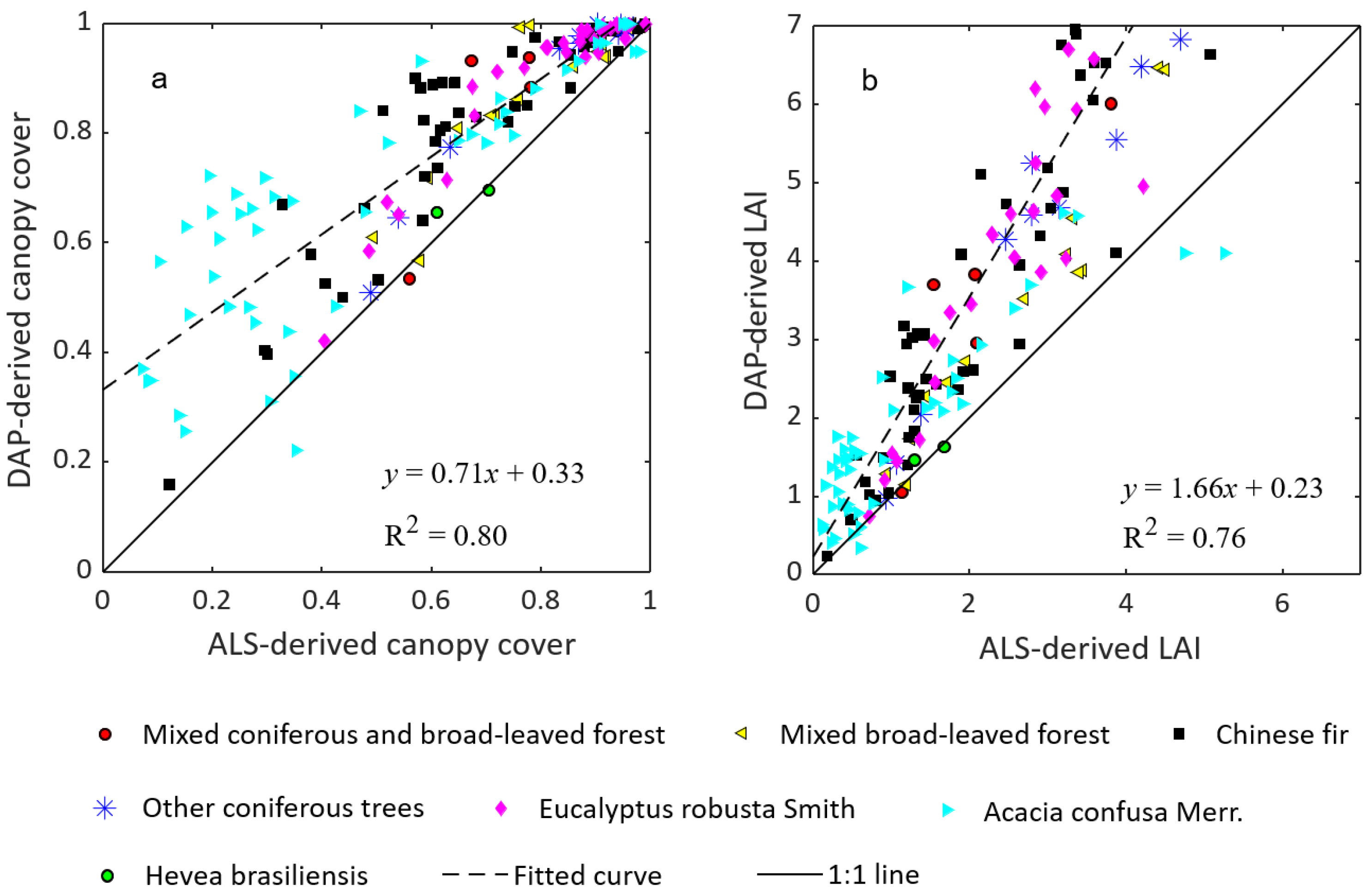
Figure 2 shows the comparisons of canopy cover and LAI estimates between the ALS-based and DAP-based methods across different species and forest types. Overall, canopy cover estimates using ALS-based and DAP-based methods showed superior correlations with a coefficient of determination (R2) of 0.80 with R2 ranging from 0.64 to 0.89 for different species. Accordingly, the LAI estimates using these two methods were also highly correlated with an R2 of 0.76 with the lowest R2 being 0.54 for the mixed broad-leaved forest and the highest R2 being 0.87 for the mixed coniferous and broad-leaved forest (Table 2). Despite the high correlations, it can be noted that almost all DAP-based estimates of canopy cover and LAI are larger than ALS-based estimates. The differences in canopy cover estimates between the two methods are not consistent across the range of canopy cover levels. Particularly, the differences are especially large in the case of low canopy cover levels. Due to the gap probability theory in the LAI estimation, the differences in LAI estimates between the two methods are large in the case of high LAI levels corresponding to the low canopy cover levels. From the perspective of forest type, there is no obvious difference in correlation between the two methods among different tree species and forest types. DAP-based canopy cover estimation tends to be closer to 1, especially for Eucalyptus robusta Smith and Acacia confusa Merr. when canopies are dense. Correspondingly, the DAP-based LAI estimates even approach 7 which represents very dense canopies in tropical forests.

4.2. Relationship between LAI and Aboveground Biomass

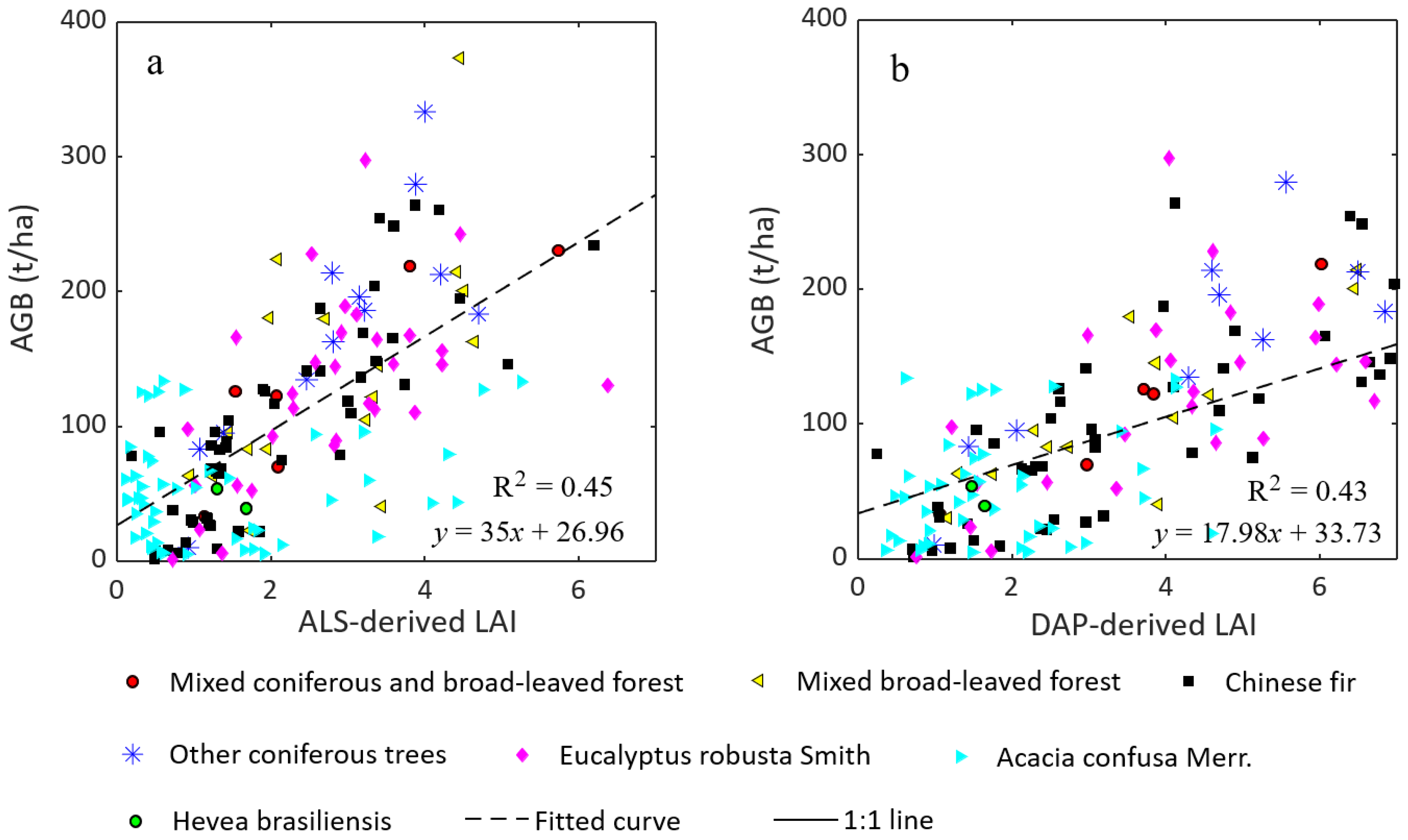
The relationship between the field-measured AGB and remote sensing-estimated LAI is shown in Figure 3. Similar correlations were found between LAIDAP–AGB (R2 of 0.43) and LAIALS–AGB (R2 of 0.45), although the correlations are relatively low. There are apparent differences in correlations among forest types (Table 3). The mixed coniferous and broad-leaved forest shows the best correlation between aboveground biomass and derived LAI with R2 larger than 0.70. For mixed broad-leaved forest, other coniferous trees, and Eucalyptus robusta Smith, R2 is around 0.50 with AGB ranging from 0 to 400 t/ha. However, for Hevea brasiliensis, there is almost no correlation between derived LAI and aboveground biomass (R2 = 0.03 for ALS and 0.01 for DAP). Derived LAI of Hevea brasiliensis is centered between 0 and 3 with aboveground biomass less than 150 t/ha. Since there are only two plots of Chinese fir, the correlation between derived LAI and aboveground biomass is not computed.

4.3. Comparison between Airborne and Sentinel-2 LAI Estimates

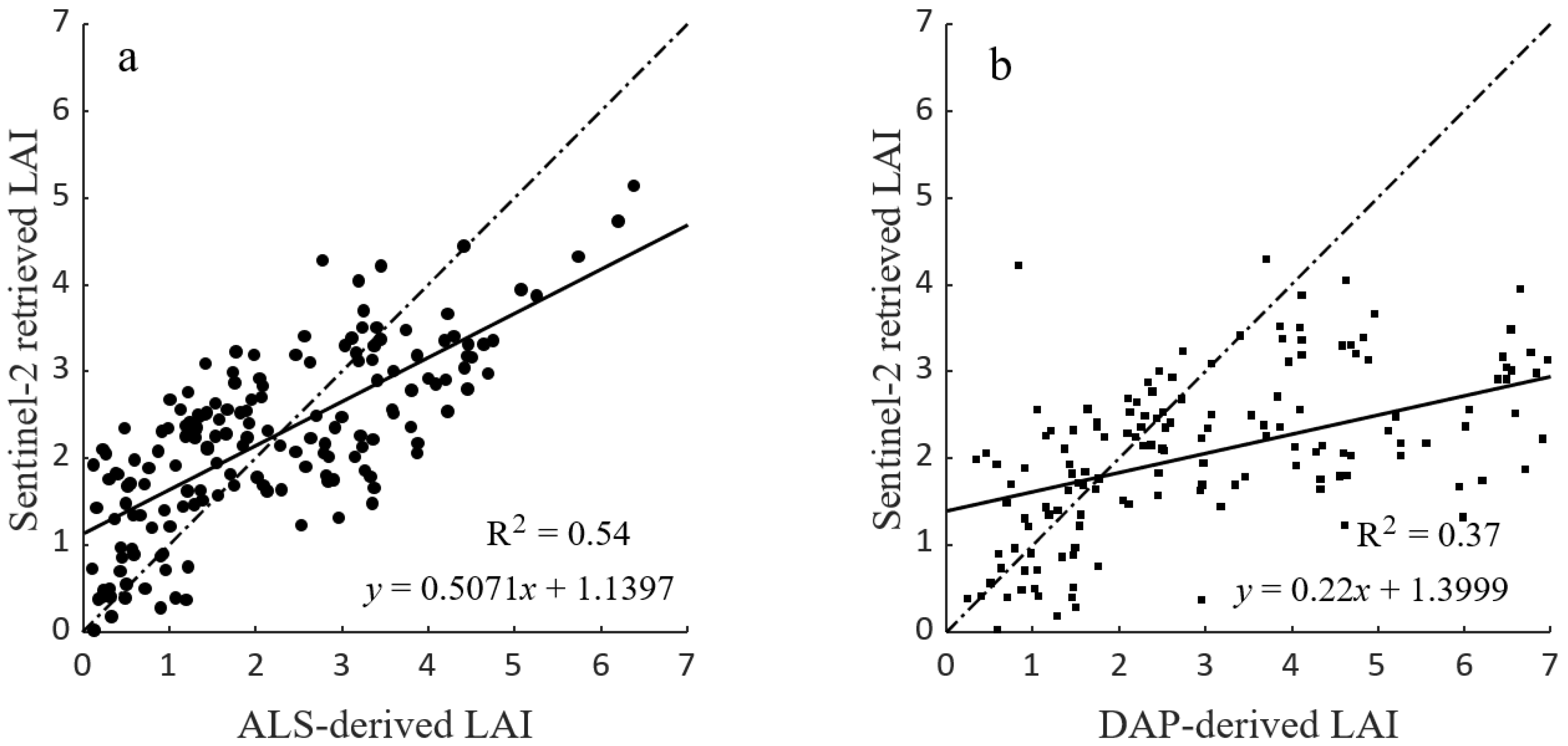
As shown by Figure 4, the ALS- and DAP-based LAI estimates were compared with Sentinel-2-retrieved LAI, respectively. The ALS results have better agreement with Sentinel-2 results with an R2 of 0.54 while DAP results show quite low correlation with Sentinel-2 retrievals. It should be noted that the Sentinel-2-based LAI estimates were obtained using a turbid medium radiative transfer model, implying no clumping effect was considered. This may explain the relatively high correlation between airborne and satellite estimates. In addition, we used a series of soil spectra obtained from a public library rather than the field measurements due to the high heterogeneity of the forest floor. The differences in LAI between ALS and Sentinel-2 are generally less than 1.5 despite the very few points falling outside this range. In contrast, the maximum difference in LAI between DAP and Sentinel-2 may be up to about 3.0.

5. Discussion

Prior to this study, the relative suitabilities of DAP and ALS data for canopy cover and LAI estimation have not been sufficiently compared. We collected DAP and ALS data of 166 tropical forest plots as well as ground-based forest inventory measurements. A CHM-based canopy cover estimation method was used based on DAP data whereas an echo index-based canopy cover estimation was used for ALS data. Both DAP- and ALS-derived LAIs were determined based on gap probability theory (also known as the Beer–Lambert law) with nadir gap fraction observation (i.e., the opposite of canopy cover). Our results indicate significant differences in the canopy cover and LAI estimation over tropical forests using ALS and DAP data, as well as different correlations with field-measured AGB.
Almost all DAP-based canopy cover estimates were larger than those using ALS-based methods, which was in accordance with findings from other studies [3,15,29]. Generally, ALS-based canopy variable estimation was recognized as a benchmarking method when no ground-based measurements were apparent [39], hence the DAP-based method tended to overestimate. This overestimation can be attributed to the characteristics of the DAP data themselves (including flight settings and camera configurations), the complexity of the forest structure, and the illumination environment [27,29]. DAP data mainly characterize the outer canopy envelope where the shadows and occlusions from surrounding trees can negatively influence the completeness of SfM point clouds. Additionally, the grid size also impacts the canopy cover estimation during the rasterization of SfM point clouds. Both the neglect of small canopy gaps and the large grid size led to the overestimation of canopy cover [32]. Compared to the CHM-based estimation using DAP data, ALS data enable the echo index (also known as light penetration index) to represent canopy cover using the echo-number-based method (i.e., the method using LiDAR echo number to derive an echo index) [33]. FCI is a widely used proxy of canopy cover although many other echo indices have been proposed in the last decade. It should be noted that FCI tends to only characterize between-crown gaps because the within-crown gaps are generally smaller than the pulse footprint, and hence may lead to overestimation [23]. Much explicit evidence indicates that effective canopy cover is overestimated in most forest stands and the estimates show a saturation effect in dense forests [40]. As we defined the canopy cover without considering the within-crown gaps, the FCI seems more adequate than other reported echo indices, such as SCI and WCI [14,41]. Our comparison demonstrated that the DAP data failed to estimate canopy cover with the same level of accuracy as the ALS data. The further investigation based on multiple forest types verified this finding.
The airborne LAI estimation accuracy is influenced by the correctness of gap fraction observations, the representativeness of leaf angle distribution, and the characterization of clumping effect regardless of wood elements (e.g., branches). Importantly, the small difference in canopy gap fraction in dense forests can lead to significant differences in LAI estimates due to the logarithmic expression in the gap probability model [5]. In this study, we assumed a spherical leaf angle distribution due to the lack of field measurements of leaf angles. This assumption might be inadequate for tropical forests because of the diversity of forest canopies. We also assumed the random spatial distribution of leaves, i.e., ignoring the clumping effect, which may cause LAI underestimation [42]. Despite the large uncertainty of ALS-based LAI estimation, it theoretically yielded more accurate estimates than the DAP-based method. We investigated the relationship between LAI and AGB over all forest plots and found relatively high correlations, especially for the mixed coniferous and broad-leaved forest. The high correlation may be partly explained by the competitive growth.
The comparison between airborne and satellite LAI estimates basically verified that the ALS-based LAI might be more reliable since they showed high consistency with the widely used Sentinel-2 retrievals using the PROSAIL model and ANN machine learning [43]. As the clumping effect was ignored in both airborne and satellite estimation, there were no apparent systematic differences in LAI between them. Some significant differences in LAI between ALS and Sentinel-2 retrievals may be explained by the topography effect because rugged terrain may cause variation in spectral reflectance. Complex forest background is another uncertainty source that contributes heterogeneous background spectral reflectance, resulting in limited representativeness when using a soil library [44]. Although DAP has proven its merit in forest inventory applications, our study showed it has relatively low capacity in canopy biophysical variable estimation, especially in LAI estimation.

6. Conclusions

This study evaluated the performance of ALS- and DAP-based methods in canopy cover and LAI estimation using many tropical forest plots. As the DAP data produced by the SfM algorithm cannot offer a detailed enough 3D canopy like ALS data, the canopy cover and the associated LAI estimates were remarkably larger than the ALS-based estimates. Differences in correlation among different forest types and tree species were also found (R2 of canopy cover and LAI range from 0.64 to 0.89 and from 0.54 to 0.87, respectively), regardless of the overall R2 of 0.80 for canopy cover and overall R2 of 0.76 for LAI. We explored the relationship between airborne LAI estimates and field-measured AGB and found better correlation between ALS-based LAI and AGB, indirectly validating the credibility of the ALS-based method. Different forest types and tree species exhibited different correlations where the optimal correlation occurred in the mixed coniferous and broad-leaved forests. The comparison between airborne and Sentinel-2-based LAI estimates again verified the value of the ALS-based method, given its better consistency with the widely used satellite-scale hybrid retrieval method. This study provides an insight on the ability of the existing 3D data in canopy variable estimation.

Author Contributions

Data curation, L.L.; Formal analysis, X.Z. and J.J.; Investigation, Y.Z.; Methodology, C.L.; Validation, F.W.; Writing—original draft, C.L. and Y.Z.; Writing—review & editing, F.W. All authors have read and agreed to the published version of the manuscript.

Funding

This research received no external funding.

Informed Consent Statement

Informed consent was obtained from all subjects involved in the study.

Data Availability Statement

Not applicable.

Conflicts of Interest

The authors declare no conflict of interest.

References

  1. Weiss, M.; Baret, F.; Smith, G.J.; Jonckheere, I.; Coppin, P. Review of methods for in situ leaf area index (LAI) determination: Part II. Estimation of LAI, errors and sampling. Agric. For. Meteorol. 2004, 121, 37–53. [Google Scholar] [CrossRef]
  2. Korhonen, L.; Korpela, I.; Heiskanen, J.; Maltamo, M. Airborne discrete-return LIDAR data in the estimation of vertical canopy cover, angular canopy closure and leaf area index. Remote Sens. Environ. 2011, 115, 1065–1080. [Google Scholar] [CrossRef]
  3. Li, L.; Chen, J.; Mu, X.; Li, W.; Yan, G.; Xie, D.; Zhang, W. Quantifying Understory and Overstory Vegetation Cover Using UAV-Based RGB Imagery in Forest Plantation. Remote Sens. 2020, 12, 298. [Google Scholar] [CrossRef]
  4. Jennings, S.B.; Brown, N.D.; Sheil, D. Assessing forest canopies and understorey illumination: Canopy closure, canopy cover and other measures. Forestry 1999, 72, 59–74. [Google Scholar] [CrossRef]
  5. Yan, G.; Hu, R.; Luo, J.; Weiss, M.; Jiang, H.; Mu, X.; Xie, D.; Zhang, W. Review of indirect optical measurements of leaf area index: Recent advances, challenges, and perspectives. Agric. For. Meteorol. 2019, 265, 390–411. [Google Scholar] [CrossRef]
  6. Smith, M.-L.; Anderson, J.; Fladeland, M. Forest canopy structural properties. In Field Measurements for Forest Carbon Monitoring; Springer: Berlin/Heidelberg, Germany, 2008; pp. 179–196. [Google Scholar]
  7. Bonan, G.B. Importance of leaf area index and forest type when estimating photosynthesis in boreal forests. Remote Sens. Environ. 1993, 43, 303–314. [Google Scholar] [CrossRef]
  8. Baret, F.; Weiss, M.; Lacaze, R.; Camacho, F.; Makhmara, H.; Pacholcyzk, P.; Smets, B. GEOV1: LAI and FAPAR essential climate variables and FCOVER global time series capitalizing over existing products. Part1: Principles of development and production. Remote Sens. Environ. 2013, 137, 299–309. [Google Scholar] [CrossRef]
  9. Watson, D.J. Comparative physiological studies on the growth of field crops: I. Variation in net assimilation rate and leaf area between species and varieties, and within and between years. Ann. Bot. 1947, 11, 41–76. [Google Scholar] [CrossRef]
  10. Myneni, R.B.; Ramakrishna, R.; Nemani, R.; Running, S.W. Estimation of global leaf area index and absorbed PAR using radiative transfer models. IEEE Trans. Geosci. Remote Sens. 1997, 35, 1380–1393. [Google Scholar] [CrossRef]
  11. Towers, P.C.; Strever, A.; Poblete-Echeverría, C. Comparison of vegetation indices for leaf area index estimation in vertical shoot positioned vine canopies with and without grenbiule hail-protection netting. Remote Sens. 2019, 11, 1073. [Google Scholar] [CrossRef] [Green Version]
  12. Jacquemoud, S.; Verhoef, W.; Baret, F.; Bacour, C.; Zarco-Tejada, P.J.; Asner, G.P.; François, C.; Ustin, S.L. PROSPECT + SAIL models: A review of use for vegetation characterization. Remote Sens. Environ. 2009, 113, S56–S66. [Google Scholar] [CrossRef]
  13. Wulder, M.A.; White, J.C.; Nelson, R.F.; Næsset, E.; Ørka, H.O.; Coops, N.C.; Hilker, T.; Bater, C.W.; Gobakken, T. Lidar sampling for large-area forest characterization: A review. Remote Sens. Environ. 2012, 121, 196–209. [Google Scholar] [CrossRef]
  14. Armston, J.; Disney, M.; Lewis, P.; Scarth, P.; Phinn, S.; Lucas, R.; Bunting, P.; Goodwin, N. Direct retrieval of canopy gap probability using airborne waveform lidar. Remote Sens. Environ. 2013, 134, 24–38. [Google Scholar] [CrossRef]
  15. White, J.C.; Tompalski, P.; Coops, N.C.; Wulder, M.A. Comparison of airborne laser scanning and digital stereo imagery for characterizing forest canopy gaps in coastal temperate rainforests. Remote Sens. Environ. 2018, 208, 1–14. [Google Scholar] [CrossRef]
  16. Fisher, A.; Armston, J.; Goodwin, N.; Scarth, P. Modelling canopy gap probability, foliage projective cover and crown projective cover from airborne lidar metrics in Australian forests and woodlands. Remote Sens. Environ. 2020, 237, 111520. [Google Scholar] [CrossRef]
  17. Dandois, J.P.; Ellis, E.C. High spatial resolution three-dimensional mapping of vegetation spectral dynamics using computer vision. Remote Sens. Environ. 2013, 136, 259–276. [Google Scholar] [CrossRef]
  18. Morsdorf, F.; Kötz, B.; Meier, E.; Itten, K.I.; Allgöwer, B. Estimation of LAI and fractional cover from small footprint airborne laser scanning data based on gap fraction. Remote Sens. Environ. 2006, 104, 50–61. [Google Scholar] [CrossRef]
  19. Hosoi, F.; Omasa, K. Voxel-based 3-D modeling of individual trees for estimating leaf area density using high-resolution portable scanning lidar. IEEE Trans. Geosci. Remote Sens. 2006, 44, 3610–3618. [Google Scholar] [CrossRef]
  20. Wang, Y.; Fang, H. Estimation of LAI with the LiDAR technology: A review. Remote Sens. 2020, 12, 3457. [Google Scholar] [CrossRef]
  21. Solberg, S.; Hill, R.; Rosette, J.; Suárez, J. Comparing discrete echoes counts and intensity sums from ALS for estimating forest LAI and gap fraction. In Proceedings of the SilviLaser, Edinburgh, UK, 17–19 September 2008; pp. 247–256. [Google Scholar]
  22. Chen, J.M.; Rich, P.M.; Gower, S.T.; Norman, J.M.; Plummer, S. Leaf area index of boreal forests: Theory, techniques, and measurements. J. Geophys. Res. Atmos. 1997, 102, 29429–29443. [Google Scholar] [CrossRef] [Green Version]
  23. Hopkinson, C.; Chasmer, L. Testing LiDAR models of fractional cover across multiple forest ecozones. Remote Sens. Environ. 2009, 113, 275–288. [Google Scholar] [CrossRef]
  24. Alonzo, M.; Bookhagen, B.; McFadden, J.P.; Sun, A.; Roberts, D.A. Mapping urban forest leaf area index with airborne lidar using penetration metrics and allometry. Remote Sens. Environ. 2015, 162, 141–153. [Google Scholar] [CrossRef]
  25. Li, D.; Gu, X.; Pang, Y.; Chen, B.; Liu, L. Estimation of forest aboveground biomass and leaf area index based on digital aerial photograph data in northeast China. Forests 2018, 9, 275. [Google Scholar] [CrossRef]
  26. Noordermeer, L.; Bollandsås, O.M.; Ørka, H.O.; Næsset, E.; Gobakken, T. Comparing the accuracies of forest attributes predicted from airborne laser scanning and digital aerial photogrammetry in operational forest inventories. Remote Sens. Environ. 2019, 226, 26–37. [Google Scholar] [CrossRef]
  27. Iglhaut, J.; Cabo, C.; Puliti, S.; Piermattei, L.; O’Connor, J.; Rosette, J. Structure from Motion Photogrammetry in Forestry: A Review. Curr. For. Rep. 2019, 5, 155–168. [Google Scholar] [CrossRef]
  28. Hernández-Clemente, R.; Navarro-Cerrillo, R.M.; Romero Ramírez, F.J.; Hornero, A.; Zarco-Tejada, P.J. A novel methodology to estimate single-tree biophysical parameters from 3D digital imagery compared to aerial laser scanner data. Remote Sens. 2014, 6, 11627–11648. [Google Scholar] [CrossRef]
  29. Li, L.; Mu, X.; Chianucci, F.; Qi, J.; Jiang, J.; Zhou, J.; Chen, L.; Huang, H.; Yan, G.; Liu, S. Ultrahigh-resolution boreal forest canopy mapping: Combining UAV imagery and photogrammetric point clouds in a deep-learning-based approach. Int. J. Appl. Earth Obs. Geoinf. 2022, 107, 102686. [Google Scholar] [CrossRef]
  30. Vastaranta, M.; Wulder, M.A.; White, J.C.; Pekkarinen, A.; Tuominen, S.; Ginzler, C.; Kankare, V.; Holopainen, M.; Hyyppä, J.; Hyyppä, H. Airborne laser scanning and digital stereo imagery measures of forest structure: Comparative results and implications to forest mapping and inventory update. Can. J. Remote Sens. 2013, 39, 382–395. [Google Scholar] [CrossRef]
  31. Li, C.; Yu, Z.; Wang, S.; Wu, F.; Wen, K.; Qi, J.; Huang, H. Crown Structure Metrics to Generalize Aboveground Biomass Estimation Model Using Airborne Laser Scanning Data in National Park of Hainan Tropical Rainforest, China. Forests 2022, 13, 1142. [Google Scholar] [CrossRef]
  32. Cai, S.; Zhang, W.; Jin, S.; Shao, J.; Li, L.; Yu, S.; Yan, G. Improving the estimation of canopy cover from UAV-LiDAR data using a pit-free CHM-based method. Int. J. Digit. Earth 2021, 14, 1477–1492. [Google Scholar] [CrossRef]
  33. Yin, T.; Qi, J.; Cook, B.D.; Morton, D.C.; Wei, S.; Gastellu-Etchegorry, J.P. Modeling Small-Footprint Airborne Lidar-Derived Estimates of Gap Probability and Leaf Area Index. Remote Sens. 2019, 12, 4. [Google Scholar] [CrossRef]
  34. Lang, M.; Kuusk, A.; Mõttus, M.; Rautiainen, M.; Nilson, T. Canopy gap fraction estimation from digital hemispherical images using sky radiance models and a linear conversion method. Agric. For. Meteorol. 2010, 150, 20–29. [Google Scholar] [CrossRef]
  35. Nilson, T. A theoretical analysis of the frequency of gaps in plant stands. Agric. Meteorol. 1971, 8, 25–38. [Google Scholar] [CrossRef]
  36. Lang, A.R.G.; Xiang, Y. Estimation of leaf area index from transmission of direct sunlight in discontinuous canopies. Agric. For. Meteorol. 1986, 37, 229–243. [Google Scholar] [CrossRef]
  37. Claverie, M.; Ju, J.; Masek, J.G.; Dungan, J.L.; Vermote, E.F.; Roger, J.C.; Skakun, S.V.; Justice, C. The Harmonized Landsat and Sentinel-2 surface reflectance data set. Remote Sens. Environ. 2018, 219, 145–161. [Google Scholar] [CrossRef]
  38. Schlerf, M.; Atzberger, C. Inversion of a forest reflectance model to estimate structural canopy variables from hyperspectral remote sensing data. Remote Sens. Environ. 2006, 100, 281–294. [Google Scholar] [CrossRef]
  39. Zhao, K.; Popescu, S. Lidar-based mapping of leaf area index and its use for validating GLOBCARBON satellite LAI product in a temperate forest of the southern USA. Remote Sens. Environ. 2009, 113, 1628–1645. [Google Scholar] [CrossRef]
  40. Arumäe, T.; Lang, M. Estimation of canopy cover in dense mixed-species forests using airborne lidar data. Eur. J. Remote Sens. 2017, 51, 132–141. [Google Scholar] [CrossRef]
  41. Solberg, S.; Brunner, A.; Hanssen, K.H.; Lange, H.; Næsset, E.; Rautiainen, M.; Stenberg, P. Mapping LAI in a Norway spruce forest using airborne laser scanning. Remote Sens. Environ. 2009, 113, 2317–2327. [Google Scholar] [CrossRef]
  42. Hu, R.; Yan, G.; Nerry, F.; Liu, Y.; Jiang, Y.; Wang, S.; Chen, Y.; Mu, X.; Zhang, W.; Xie, D. Using Airborne Laser Scanner and Path Length Distribution Model to Quantify Clumping Effect and Estimate Leaf Area Index. IEEE Trans. Geosci. Remote Sens. 2018, 56, 3196–3209. [Google Scholar] [CrossRef]
  43. Fernández-Guisuraga, J.M.; Verrelst, J.; Calvo, L.; Suárez-Seoane, S. Hybrid inversion of radiative transfer models based on high spatial resolution satellite reflectance data improves fractional vegetation cover retrieval in heterogeneous ecological systems after fire. Remote Sens. Environ. 2021, 255, 112304. [Google Scholar] [CrossRef] [PubMed]
  44. Li, L.; Mu, X.; Qi, J.; Pisek, J.; Roosjen, P.; Yan, G.; Huang, H.; Liu, S.; Baret, F. Characterizing reflectance anisotropy of background soil in open-canopy plantations using UAV-based multiangular images. ISPRS J. Photogramm. Remote Sens. 2021, 177, 263–278. [Google Scholar] [CrossRef]
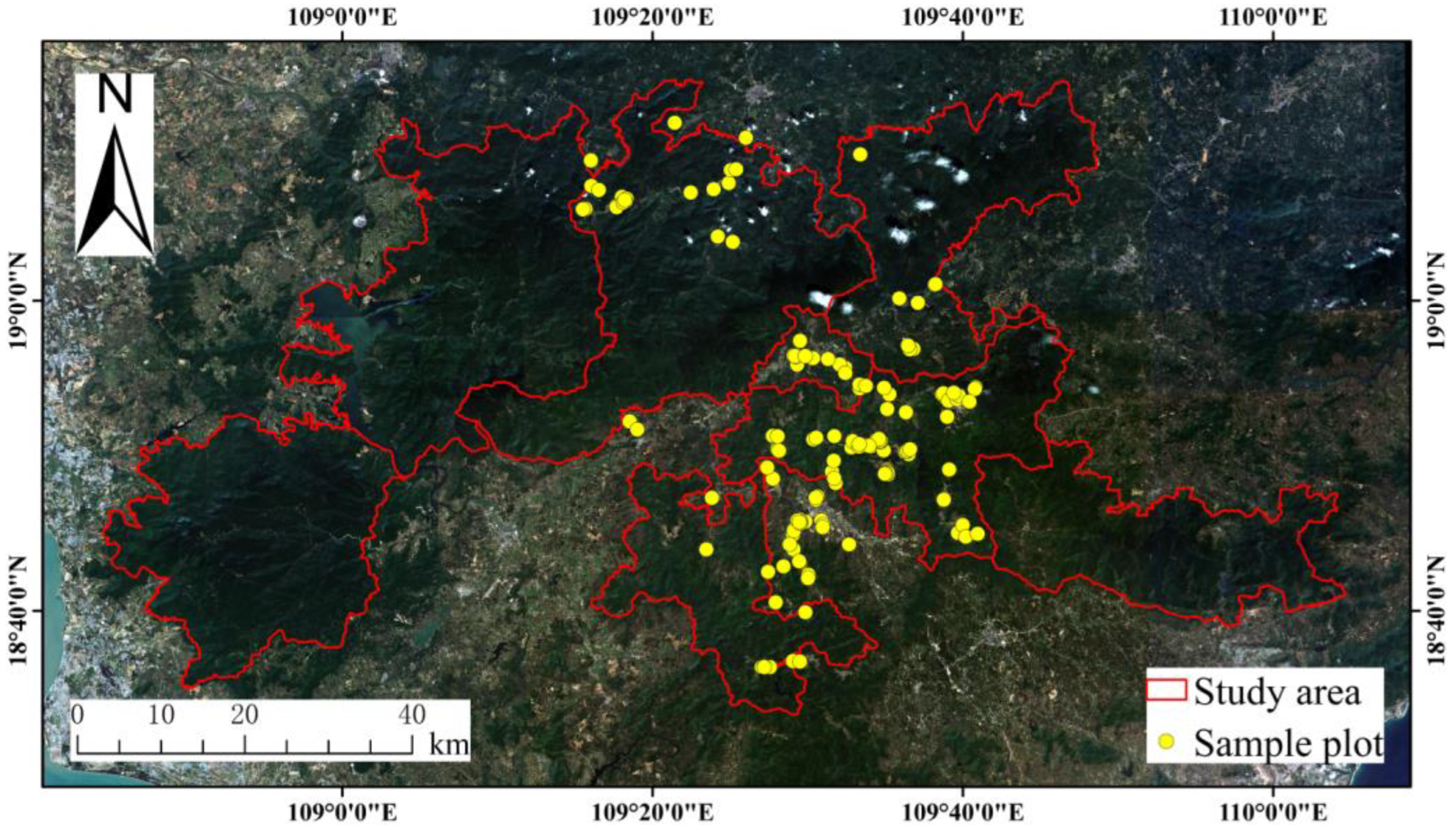
Figure 1. Study area in the Hainan national tropical rainforest park with the background being a Sentinel-2 true color image. Yellow dots refer to the forest sample plots in the field inventory.
Applsci 12 09882 g001
Figure 2. Comparison of canopy cover (a) and leaf area index (LAI) (b) between DAP-based and ALS-based estimation methods across different forest types.
Applsci 12 09882 g002
Figure 3. Correlation between ALS-derived LAI and aboveground biomass (AGB) (a), between DAPS-derived LAI and AGB (b) for different forest types.
Applsci 12 09882 g003
Figure 4. Comparison between airborne and satellite-retrieved leaf area index (LAI), with ALS-based LAI against Sentinel-2-based LAI (a), and with DAP-based LAI against Sentinel-2-based LAI (b).
Applsci 12 09882 g004
Table 1. Allometry equations of aboveground biomass (AGB) of individual trees for different tree species and forest types. D and H represent the DBH and tree height, respectively.
Tree Species and Forest TypesAllometry Equation of Individual TreeAGB of Plot (t/ha)
Coniferous and broad-leaved mixed forest A G B = 0.2253 × D 2.4213 124.6   ±   106.4
Broad-leaved mixed forest A G B = 0.1131 × D 2 H 0.8407 113.5   ±   260.2
Other coniferous trees A G B = 0.2309 × D 2 H 0.6838 185.0   ±   174.6
Chinese fir A G B = 0.0182 × D 2 H 0.9710 46.8   ±   7.3
Eucalyptus robusta Smith A G B = 0.0576 × D 2 H 0.8587 89.2   ±   175.3
Acacia confusa Merr. A G B = 1.4240 × D 2 H 0.5680 127.6   ±   170.0
Hevea brasiliensis A G B = 0.0524 × D 2.7451 46.5   ±   87.7
Table 2. Coefficients of determination (R2) of fitted curves between DAP-based and the ALS-based estimated canopy cover and LAI under different forest types.
Coefficients of DeterminationCanopy CoverLAI
Mixed coniferous and broad-leaved forest0.640.87
Mixed broad-leaved forest0.790.54
Other coniferous trees0.940.66
Eucalyptus robusta Smith0.810.84
Acacia confusa Merr.0.890.82
Hevea brasiliensis0.710.67
All0.800.76
Table 3. Coefficients of determination (R2) of fitted curves between field-measured aboveground biomass (AGB) and the estimated LAI using ALS and DAP methods under different forest types.
Coefficients of DeterminationLAIALS–AGBLAIDAP–AGB
Mixed coniferous and broad-leaved forest0.770.96
Mixed broad-leaved forest0.390.65
Other coniferous trees0.670.55
Eucalyptus robusta Smith0.670.63
Acacia confusa Merr.0.300.24
Hevea brasiliensis0.030.01
Publisher’s Note: MDPI stays neutral with regard to jurisdictional claims in published maps and institutional affiliations.