Abstract
The population of satellites in Low Earth Orbit is predicted to growth exponentially in the next decade due to the proliferation of small-sat constellations. Consequently, the probability of collision is expected to increase dramatically, possibly leading to a potential Kessler syndrome situation. It is therefore necessary to strengthen all the technologies required for collision avoidance and end-of-life disposal of new satellites, together with active debris removal of current and potential future dead satellites. Both situations require the lowering of the altitude of a satellite up to re-entry. In this paper several de-orbiting technologies are evaluated: natural decay, chemical propulsion (solid and liquid), electric propulsion, drag sail, electrodynamic tether, and combinations of the previous ones. The comparison considers the initial altitude, system mass, de-orbiting time, collision probability during descent, reliability, and technological limits. Differences between active debris removal and satellite end-of-life self-disposal are taken into account. Moreover, the different types of re-entry, controlled vs. non-controlled, expendable vs. reusable system, demisable vs. non-demisable system are also discussed. Finally, the possibility to operate the satellite in Very Low Earth Orbits with a propulsion system for drag compensation and passive re-entry at end of life is investigated.
Keywords:
de-orbiting; end-of-life disposal; space debris; propulsion; tether; sail; orbital decay; LEO; VLEO; drag compensation 1. Introduction
In recent times there has been an increasing concern about debris in Low Earth Orbit (LEO); in fact it is more and more frequent to find in the space-related news episodes of collision avoidance or sometimes even real (deliberate or unwanted) collisions or fragmentations of space objects [1,2]. This is due to the fact that the satellite population in LEO is growing exponentially as the number of satellites put into orbit is much greater than quantity of the ones that are removed. Moreover, actual predictions of future space trends show a further order of magnitude increase due to the rise of the so-called mega-constellations [3,4]. Space experts, shareholders and institutions all around the world have often claimed that the current behavior cannot be tolerated as it is in the future, otherwise the possibility of Kessler syndrome with its consequent terrible effects could become real [5,6]. Even without a catastrophic scenario, a crowded space environment could render it more difficult to operate in space, as, for example, a significant number of collision avoidance maneuvers could impact the delta-v budget of the mission and the cost of operations. Therefore, it is necessary to take actions in order to limit as much as possible the amount of inoperative material orbiting in LEO. At these altitudes, the common way to clean the orbits is trough deorbiting and re-entry/disintegration of the space object.
It is worth noting that the largest portion (around 2/3) of orbital debris is concentrated in LEO, and that only 6% of Earth orbiting objects are operational payloads [7,8]. Moreover, LEO altitude distribution shows a peak around 800 km, which is in fact one of the favorite orbital altitudes and the target of the new small-sat rideshare launch missions like the recent Transporter service by SpaceX [9].
There are plenty of important aspects related with space debris like monitoring, prediction, traffic management, protection, policy, autonomous detection, operations and so forth [10,11,12,13,14]. This paper will focus only on a single, unavoidable aspect, the means for de-orbiting satellites at the end of life. This topic has been already discussed previously [15,16,17,18], and many numerical methods for the solution of the perturbed two-body problem have been developed, e.g., [19,20,21]. However, here some new further-simplified analyses will be shown, with a specific focus on the system level impact of the added devices, in particular total mass and deorbiting time.
Generally, the principal proposed ways to deorbit a satellite are the natural aerodynamic decay (sometimes with a drag-boosting device, i.e., a drag sail), propulsive de-orbit, electrodynamic tethers, solar sails.
Compared to previous works [15,16,17,18], the range of the initial conditions for the comparison (altitude, decay time, inclination, duty cycle, deorbiting profile etc.) has been extended. Moreover, the combinations between different technologies will be also discussed. Finally, the paradigm of drag compensation will be directly compared with conventional deorbit. Other aspects closely related with deorbiting will be also reviewed.
The aim of this work is to better understand the different available options with their strength and weaknesses and provide simple tools, guidelines and warnings in order to support future selections or developments.
2. Deorbiting Technologies
The simplest way to deorbit a satellite in LEO is using the natural aerodynamic decay. This is a passive and inexpensive solution. However, the drag D produced is linearly dependent on the atmospheric density ρ:
The drag coefficient cd is considered near 2 for a typical satellite (2.2 used in this paper), where A is the frontal area respect to the incoming flow (the opposite of the velocity vector). Here the density has been calculated with the US Standard Atmosphere 1976 model, USSA1976 [22]. This model does not take into account temporal and horizontal spatial variations, but only the average behavior with altitude. More complete models are available [23], and it is important to remember that the actual density at a certain altitude can change significantly due to variations in Sun activity. However, once this caveat is known, the current model anyway is considered sufficient to be used for the relative comparison of the different deorbiting technologies.
The atmospheric density has roughly an exponential behavior with altitude. Therefore, the lifetime of a dead satellite is also an exponential function of the altitude. Current legislations foresee a decay time below 25 years for non-operational satellites. It is possible to see that the corresponding limit altitude is around 600 km. It is worth remembering that the peak of debris and the current favorite altitude is slightly above this value. However, from the current analyses and trends it is possible to predict (and also to encourage) that sooner or later the legislation should become stricter, reducing the time allowed to complete deorbit. In this case the limit altitude will decrease significantly. The author proposes the possibility to put a mandatory fee on deorbit, with the fee proportional to the deorbit time, or time spent in orbit after end of life in case of failed deorbit (forcing an active debris removal in the latter).
In order to improve the decay time, it is possible to add a drag sail [24,25,26,27,28]. This device is deployed at the end of life to drastically increase the frontal area and consequently the drag, therefore reducing the deorbit time. The device needs an actuation system, i.e., a mechanism to deploy the sail correctly and a communication link or an internal computer that starts the procedure when needed. Consequently, at least two failure points are introduced.
The mass of the drag sail is approximated as a linear function of its area. Typical values of area density are around 75 g/m2 with up to dozens of m2 of area [17]. After deployment, the satellite will theoretically passively deorbit. However, in the general case the attitude of the satellite could change with time and the drag sail could not present its full area against the flow, reducing its efficacy. Three possibilities are then possible: to accept a performance degradation, but this choice is not preferable as it comes with a significant uncertainty; to add an attitude control during re-entry, perhaps using one already present in the satellite (which, however should cope with different forces compared to its original design requirements); or, finally, find a suitable sail shape design that would preserve its positional stability with respect to the incoming flow. The last possibility seems the most promising, even if not fully developed.
However, the drag sail linearly decreases the decay time as the inverse of its frontal area. Therefore, it performs very well at low altitudes, but rapidly loses effectiveness at higher altitudes.
A similar solution is the solar sail. The solar sail is a proposed solution to impart a delta-v on a spacecraft without consuming propellant, but rather using the force from solar radiation. Very interesting for certain missions, it can be potentially used also for deorbiting a spacecraft. The solar pressure is:
where I is the solar irradiance and c the speed of light [8]. The value of the solar pressure is rather low, around 4.5 μN/m2. The altitude at which the solar and aerodynamic pressure are equal is around 600 km. At this altitude, the drag sail is already not the best-performing solution, thus the solar sail is not well suited for deorbit, particularly taking into account that the solar vector is not aligned with the opposite of the velocity vector for most of the orbit (unlike aerodynamic drag), thereby dramatically reducing its effectiveness and requiring an active attitude control to properly orient the sail.
The classical way to deorbit a satellite is to use a propulsion system. The parameters characterizing the propulsion system are the specific impulse Isp, thrust T, total impulse Itot, propellant mass mp. The propellant mass is dependent on the delta-v (∆v) required for deorbiting trough the Tsiolkovsky equation:
where the subscripts i and f stand for initial and final, respectively. For high-thrust systems, an impulsive maneuver can be considered and a Hohmann transfer from the original orbit to another at lower altitude with corresponding lower lifetime can be performed.
where a stands for apogee, p for perigee, H for Hohmann and v is the instantaneous orbital velocity:
Which is constant for a circular orbit. μ is the Earth gravitational constant, r the local orbit radius and a is the semi-major axis. Required delta-v and thrust are generally sufficiently high to force the use of a chemical propulsion system, which are divided between solids, liquids and, less frequently, hybrids.
Solid systems have the advantage to be very compact and simple, favoring a dedicated one-shot device [29,30,31]. Metallized solid propellants release solid particles, so less energetic particle-free formulations are preferable, particularly for deorbit from high altitudes. Solid rockets have relatively high thrusts, which can be an issue for attitude control; in fact, often the motor requires an active thrust vector control, or the spacecraft needs to be spun during firing. Solid rockets are not suited for multifunctional use. On the contrary, liquids tend to be more complex and bulkier, but can be integrated in order to provide other propulsive functions other than deorbiting (like orbit raising and station keeping). Thrust is relatively low so attitude (and trajectory) control is much easier and precise. Hybrid propulsion has its own peculiarities as described in [32,33,34,35] and has been proposed for active deorbiting of large items [36,37].
For low-thrust systems, a continuous thrusting phase is necessary. The delta-v is the difference between the original (marked with 0) orbital velocity and the final one.
In LEO, the orbits always have a small altitude compared with the Earth radius and consequently a very low eccentricity. Therefore, the difference between a Hohmann transfer and a continuous transfer becomes negligible. The ratio between the continuous delta-v and the impulsive (Hohmann) one is given by the following equation [38]:
The ratio is only 0.32% higher than one for a deorbiting from 2000 to 300 km (828.2 m/s vs. 825.6 m/s). It is worth noting that, for altitudes above 1400 km, it is more efficient to move the satellite into a disposal orbit slightly above 2000 km than deorbit it [11].
However, thanks to the exponential behavior of the atmospheric density, instead of lowering all the orbit to a new altitude, it is possible to decrease only the perigee to an altitude slightly below the one necessary for a circular orbit to obtain the same decay time. The first half of a Hohmann transfer is roughly one-half of the total delta-v. The delta-v for this option is slightly above one half of the complete Hohmann for the same decay time. This option is possible only for a high-thrust system that can perform an impulsive maneuver. Low-thrust systems are generally of electric type, require power and are consequently limited in thrust by it. The maneuver time is generally non-negligible or even comparable with the decay time, and in fact the two are superposed. The advantage of the electric system is a much higher specific impulse that can provide an attractive mass saving for high delta-v.
Finally, the last option is the electrodynamic tether [17,39,40,41]. In this case a tether is deployed for re-entry. Electrodynamic tethers collect ionospheric electrons from the plasma environment and re-emit them through a cathode or a “Low-Work-Function” segment of the same tether by using thermionic and photoelectric effects. In both configurations, the resulting electric current flowing through the conductive tether generates a drag Lorentz force thanks to interaction with the Earth’s magnetic field. The drag force is rather small, and the deorbiting behavior is very similar to that of an electric thruster, but without propellant consumption. The technology is still not as mature as the classical propulsion; concerns arise regarding the oscillation stability of the tether–satellite system, the probability/consequences of debris impact on the tether and other engineering issues.
The Lorentz drag force Fet is described by the following equation:
where Bm is the geomagnetic field, Em the motional electric field, iav the dimensionless averaged current along the tether, m the tether mass, ρ its density, σ is the tether conductivity. Typical values are ρ = 2700 kg/m3, I = 3.54 × 10⁷ Ω−1m−1, Bm = 0.3 Gauss, iav = 0.25. For a fixed technology, the main parameters affecting the Lorentz drag force are the area and thickness of the tether and the orbital inclination i. The tether becomes less effective approaching polar orbits due to the cos2 dependency.
The average TRL of the tether systems is the lowest between all the possible options, anyway some devices are already sold as COTS on the market [42,43,44]. However, performance from datasheet seems to indicate a much higher relative auxiliary mass compared with literature projections. This is probably due to the small size of the devices and or to some compromises necessary to field such a new technology nowadays. The tether can be used also in reverse mode as a propulsion system for orbit raising (requiring power from the spacecraft), however the TRL of the technology is even lower in this case.
The chemical thruster is an active system that requires the satellite to be effective only for a limited time after the start of the disposal maneuver, generally no more than several hours in case the apogee burn is split in several smaller impulses. On the contrary, both the electric thrusters and the tethers need to work reliably for a long time, meanwhile requiring the satellite to control its attitude and basic functions, increasing the probability of failure.
Comparing the forces produced by the various technologies for 10 kg of device mass we obtain the results presented in the following Figure 1. The thrust of a chemical propulsion system is not represented as it is out of scale and not a particular limiting factor. For the electric propulsion only the fixed mass of the thruster is considered, i.e., the propellant mass is excluded as it depends on the specific altitude change. For the electric thruster the mass is computed as a linear function of the required power (mt = αP, P = 0.5T Isp g0/η), considering α = 20 kg/kW and a thruster efficiency η of 0.65.
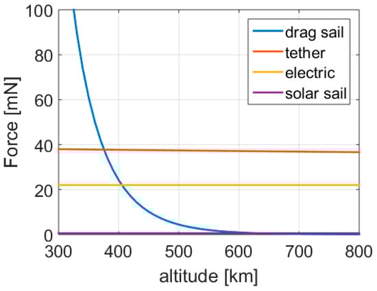
Figure 1.
Comparison of different forces produced by different deorbiting devices (10 kg mass) as a function of altitude.
The force of the drag sail is almost an exponential function of the altitude (as the atmospheric density). The thrust of the electric propulsion system is independent of the altitude. The force of the tether is calculated for a 45° orbital inclination, it is rather constant with altitude (slightly decreasing, <10% in LEO) and it is almost double that of the electric thruster. The solar sail force is negligible compared to the other devices (except when the drag sail loses usefulness), thus it is not considered a viable option. Therefore, for the rest of the paper, the term sail will be associated with aerodynamic drag sail. The drag sail is the most effective at very low altitudes while the tether is potentially the most performing solution at the majority of altitudes.
Comparing the tether with the electric propulsion system (as it is the most similar) for different inclinations for 10 kg of device mass, we obtain the results presented in Figure 2. In this case, for the electric propulsion system the propellant mass together with its corresponding structural mass m = (1 + k)mp, k = 0.12, have been also included considering a deorbiting from 750 to 200 km. It is possible to see that the superiority of the tether vanishes approaching the polar orbit and remains below the electric thruster for a sun-synchronous orbit, which is, at the moment, one of the most frequent in LEO.
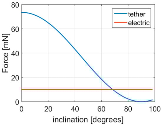
Figure 2.
Variation of the tether force with orbital inclination (10 kg mass device).
3. Materials and Methods
In order to compare the different technologies, it is necessary to calculate the deorbiting behavior. For this a simple Hohmann transfer Equation (5) is used. For a half Hohmann transfer only the first term is necessary. Propellant mass is calculated with Equations (3) and (4).
Time for the maneuver can be calculated by simple orbital mechanics [45,46,47] as half the orbital period T:
but is definitely negligible (around 90 min per each full orbit, the number of orbits depending on the number of impulses that composes the total impulse required) with respect to the typical required deorbiting time.
For the calculation of deorbiting time with drag and small forces, the equation of motion is integrated with time:
where aF is the force-induced acceleration (F/m). This is the so-called Cowell approach. It requires a small timestep in order to avoid a large error buildup. The vectorial equation is integrated with an adaptive step 4th–5th-order Runge–Kutta scheme. The error tolerance has been set by repeating the simulation until the relative error between the last two was well below 1%. For the sake of simplicity, the rotation of the atmosphere has been neglected in this work so that the relative velocity is equal to the spacecraft absolute velocity.
Two semi-analytical techniques have been also used to drastically reduce the computational time. In case of an initial circular orbit and a slow spiraling down the following equation has been used:
where t ≤ T is the time considered for integration. For elliptical orbits the following approach has been used instead. We assume that a is almost constant during one orbit:
The energy decay during one orbit is equal to the work of the forces applied to the spacecraft:
Which in case of drag:
where Bc is the ballistic coefficient:
Substituting in Equations (14) and (15):
The instantaneous velocity is:
where r means radial, t tangential, e is the eccentricity and θ the true anomaly and:
As the eccentricity is small the higher terms on e have been neglected, considering:
where E is the eccentric anomaly. Substituting in Equation (18):
Also considering Equation (20):
Remembering that:
We obtain:
Using a simple exponential atmospheric model:
where h is the altitude and H the scale height. Remembering that:
We obtain:
Substituting in Equation (25):
With:
Again, neglecting the highe-order terms on e:
Thus:
Considering the modified Bessel functions of the first kind:
we obtain:
Repeating the process same process:
The accuracy of the whole model is mainly dependent on the density model. As the atmospheric density is not a perfect exponential, the value of H changes with altitude. The value of H can be calculated from the actual density values at two different altitudes. In the following Figure 3, H is plotted as a function of the altitude for three different spacings (i.e., altitude difference) of the sampling points.
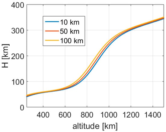
Figure 3.
Atmospheric scale factor as a function of altitude, parametric with the distance between sampling points.
The value of H is strongly dependent on the altitude and much less on the spacing between sampling points.
It is important to compare the density calculated with the current model with the original one from the USSA1976 and infer the corresponding error. Figure 4 shows the error for the case of 10 km (a) and 100 km (b) distance between the sampling points. The X-axis represents the distance from the lowest sampling point, while the curves are parametric to the altitude of the lowest sampling point (from 250 to 1500 km). It is possible to see that the exponential density model is obviously correct at the two sampling points (the points 0 and the point + 10 km or +100 km), but it overestimates the density between the two sampling points and underestimate the density above the highest sampling point. As expected, the error is larger at low initial altitudes as the density curve is steeper and the altitude variation is higher as a percentage of the initial altitude.
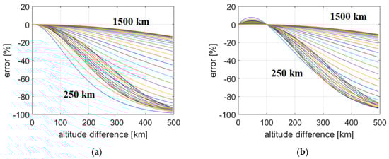
Figure 4.
Error of the exponential density model compared with the USSA1976 for: (a) 10 km sampling spacing; (b) 100 km sampling spacing. Parametric with initial altitude (250 to 1500 km at 25 km steps).
As the model is exponential, a slight error on the curve slope means that the density ratio between the estimated value and the actual one approach zero and the error asymptotically goes to −100%. Even if this error could seem apparently high, for our proposes it is important to underline the following aspect. To determine the decay of the spacecraft, it is important to correctly estimate the energy lost due to the atmospheric drag. Therefore, the accuracy near the perigee, where the drag is high, is very important, while the need for accuracy at the apogee is almost negligible.
For this reason, if someone sets a very small sampling distance, the density calculated with the simplified model will be almost always underestimate along the orbit, and the predicted decay time will be longer, but the error on the decay time will still be reasonable as the error is very small near the perigee. If the distance of the sampling points is increased, the overestimation of the density near the perigee will decrease the decay time, while the underestimation at high altitude will still increase it. After a series of trial and errors, it has been assessed that a sampling distance around 50 km gives generally the best results (Figure 5), with the two effects almost cancelling each other and the decay time prediction becoming precise in the order of an error of several percent.
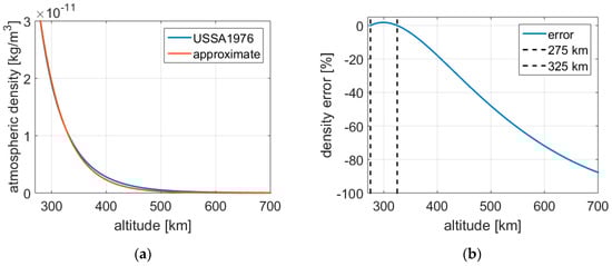
Figure 5.
Comparison between the USSA1976 density model and approximate exponential model: (a) density vs. altitude; (b) error with altitude of the exponential model for a 50 km sampling spacing.
For example, as shown in Figure 6, for the natural decay of a 50 kg satellite with 400 kg/m3 density from an initial elliptical orbit with 275 km perigee and 700 km apogee, the predicted deorbit time with the integration of the equations of motion is 347 days, while with the approximated model (50 km sampling distance) is 349 days (0.6%). Such an accurate prediction comes with a dramatically reduction in computational time.
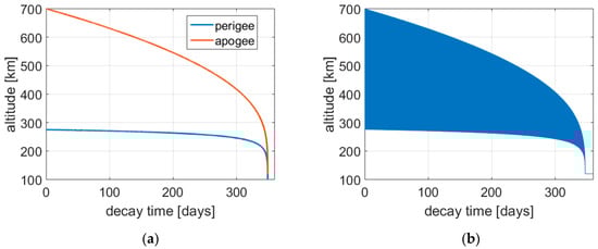
Figure 6.
Natural orbital decay from an initial elliptical orbit (275 × 700 km): (a) approximate model; (b) numerical integration of the equations of motion.
Figure 7 shows that the variation of the semi-major axis during one orbit is negligible and that the eccentricity is very low, justifying the corresponding hypotheses. It is also worth noting from Figure 8 that the flight-path angle is very small in LEO, as any elliptical orbit has a very low eccentricity anyway.
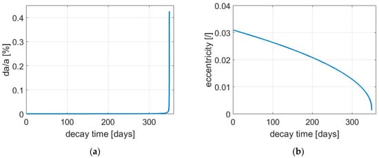
Figure 7.
Orbital decay calculated with the approximate model: (a) relative variation of the semi-major axis for each orbit; (b) eccentricity evolution with time.
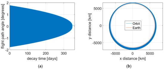
Figure 8.
Natural orbital decay from an initial elliptical orbit (275 × 700 km) calculated through the numerical integration of the equations of motion: (a) flight-path angle; (b) orbits’ shape.
Consequently, the direction of the spacecraft velocity is almost perfectly orthogonal to the instantaneous orbit radius even far from the apsides and, therefore, gravitational losses are negligible even for a continuous thrusting system.
4. Results
With the simple numerical tools described in the previous chapter it is now possible to determine the specific behavior of the different deorbiting technologies.
4.1. Natural Decay
First of all, as a reference, it is important to determine the natural decay of a typical satellite into LEO without the use of a specific device.
The decay time mainly follows the (inverse) behavior of density with altitude, so it is exponentially longer as the altitude increases (Figure 9). Moreover, the natural decay accelerates as the altitudes decreases, so the majority of the time is spent near the original altitude and the majority of the fall happens near the end of the decay time (Figure 10). This means also that in the case of deorbiting with a special device like a chemical thruster, the majority of the reduction in decay time is obtained in the initial part of the altitude decrease.
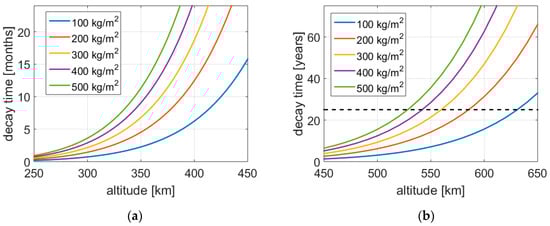
Figure 9.
Natural decay time as a function of altitude, and parametric with spacecraft mass-to-area ratio: (a) lower altitudes; (b) higher altitudes, black line is the 25 years limit.
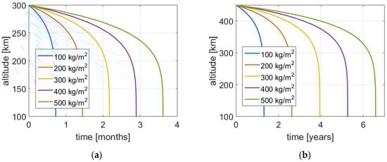
Figure 10.
Natural decay of a satellite with time, and parametric with spacecraft mass-to-area ratio: (a) 300 km initial altitude; (b) 450 km initial altitude.
The decay time is also linearly dependent on the ballistic coefficient, which is mainly determined by the ratio between the mass and the frontal area of the satellite. This ratio depends on the scale and the design of the system. For the same, identical satellite (shape and density), the scale should change the ballistic coefficient as the volume to ratio, i.e., a power of 3/2 times the linear size of the system. However, small satellites have typically higher density (around 1000–2000 kg/m3 for a cubesat) than the larger ones (even below 100 kg/m3, like the Hubble Space telescope), which mitigates the scale effect. Thus, the majority of satellites have a mass-to-area ratio between 100 and 500 kg/m2 (0.01 to 0.002 m2/kg). Anyway, specific designs with large, deployable surfaces can have very low ballistic coefficients, while in the opposite circumstances other designs elongated in the direction of the flow aimed at low-altitude flying (like GOCE [48]) can have a particularly high ballistic coefficient.
From Figure 9, it is possible to see that the 25-year limit is achieved around 500–650 km, while a re-entry in less than five years necessitates an altitude below 300–400 km. Figure 9 and Figure 10 consider circular orbits and the natural decay corresponds to a spiraling down of the satellite trajectory where the eccentricity remains negligible.
The almost exponential trend of the atmospheric density with altitude has a dramatic influence on deorbiting behavior. In the case of an elliptical orbit, the peak of drag at the perigee induces a strong reduction of the apogee altitude in a process of circularization. When the eccentricity becomes very small, the perigee starts to fall as the apogee and the orbit begin spiraling down.
The deorbiting time depends on the orbital energy and the energy dissipation. The first parameter is related to the orbit semi-major axis, while the second is strongly related with the minimum (i.e., perigee) altitude.
In Figure 11 it is possible to see that the same spacecraft has nearly the same decay time (around 2 months) for a more energetic orbit with a lower perigee (a = Rt + 450 km, hp = 200 km, ha = 700 km) and a less energetic circular orbit (h = 316 km). This is due to the fact that the first, more energetic orbit experiences a larger energy dissipation driven by the higher drag at the (lower) perigee.
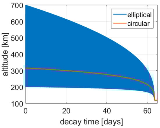
Figure 11.
Altitude vs. time for an elliptical orbit (200 × 700 km) and a circular orbit (316 km).
4.2. Drag Sail
Considering the drag sail, it is possible to plot the predicted decay time as a function of the altitude for different ratios of the sail device mass to the spacecraft total mass (Figure 12). The behavior is exactly the same of the natural decay with a simple boost of effectiveness. As already said, due to the exponential behavior of atmospheric density, the decay time becomes too long at higher altitudes. A relatively light system can shift the 25-year limit to over 1000 km. In order to further decrease the decay time, it is necessary to increase the drag sail area, and consequently mass. However, technical feasibility and operational reliability become more and more doubtful. In this case, a chemical propulsion system or a combination of a drag sail with the satellite propulsion system (often already present for other mobility needs) seems to represent a better choice.
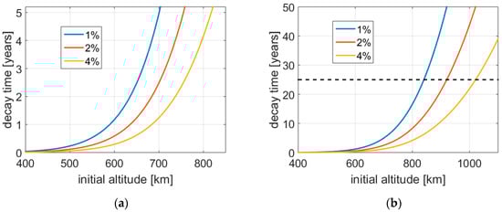
Figure 12.
Decay time as a function of altitude for three different drag sail mass fractions: (a) lower altitudes; (b) higher altitudes, with black line being the 25-year limit.
Sometimes, it is argued that the reduction in the decay time of a drag sail is proportional to its area, and that consequently the probability of impact remains unchanged. This is formally correct, but some aspects should be considered:
- The impact of small debris with the sail has probably fewer effects and consequences than an impact with the satellite;
- In case of cooperative systems, a collision avoidance process can occur [49]. This maneuver is based on an uncertainty area of impact that is much larger than the satellite itself and is thus not a linear (but rather sublinear) function of the satellite area. So, while the probability of passive impact remains constant, the probability of a collision avoidance maneuver by a third party is definitely reduced as the falling time is shortened;
- It is much easier and cheaper to track a large falling satellite for a shorter time (with the sail) than its original, way smaller, counterpart for a much longer time.
Thus, the drag sail remains an interesting option for deorbiting purposes.
For an elliptical orbit with a low perigee (perhaps as a consequence of an active partial deorbit with a chemical system, as shown in Section 4.7 about combined solutions), we think it is possible that the drag sail could be opened near the perigee to exploit the region of peak drag, and closed in the rest of the orbit where this is little effective. In this way, the probability of impact is widely reduced. However, this solution is probably not worth the added complexity and risks of having an active solar sail be deployed and closed repeatedly once every orbit.
4.3. Chemical Propulsion
With a chemical propulsion system, it is possible to perform a Hohmann transfer from the original orbit to a parking orbit with a defined natural decay time. The mass of the propulsion systems mainly depends on the propellant mass that in turn follows the delta-v between the two orbits. Chemical propulsion has the advantage of being a very fast disposal option, with the Hohmann transfer requiring half an orbit (around 45 min in LEO) for a single impulsive maneuver, or several hours in case the perigee lowering and the final orbit circularization are divided in several burns due to limitation in thrust (and consequently maximum time spent at the apsides).
Figure 13, Figure 14, Figure 15, Figure 16, Figure 17 and Figure 18 have been computed with k = 0.12 and Isp = 300 s. For delta-v up to 500 m/s and Isp = 300 s, propellant mass is almost linear with delta-v (10% error). Chemical propulsion allows satellites to deorbit from any altitude; however, the required mass can be significant, and easily represent more than 10% of the total satellite mass.
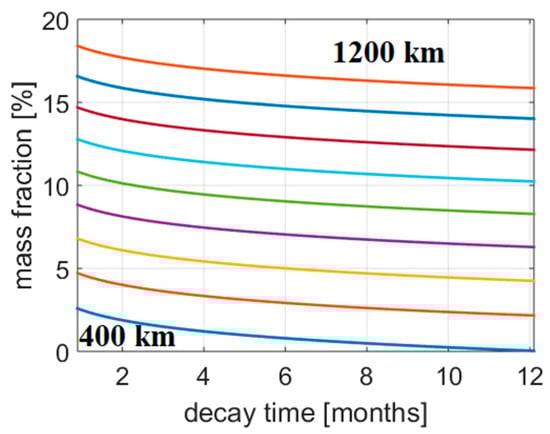
Figure 13.
Deorbiting with chemical propulsion with a full Hohmann transfer, parametric with initial altitude (400–1200 km). Propulsion system mass fraction vs. decay time.
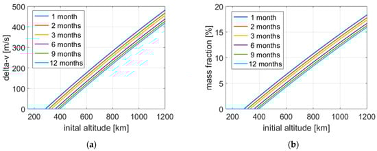
Figure 14.
Deorbiting with chemical propulsion with a full Hohmann transfer, parametric with decay time: (a) delta-v; (b) propulsion system mass fraction.
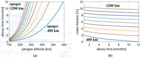
Figure 15.
Deorbiting with chemical propulsion with a half Hohmann transfer, parametric with initial altitude (400–1200 km): (a) decay time vs. perigee altitude; (b) propulsion system mass fraction vs. decay time.
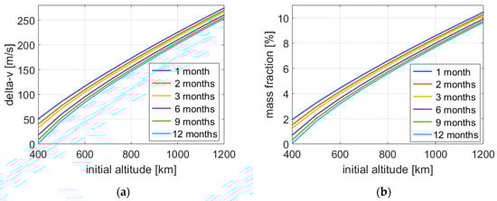
Figure 16.
Deorbiting with chemical propulsion with a half Hohmann transfer, parametric with decay time: (a) delta-v; (b) propulsion system mass fraction.
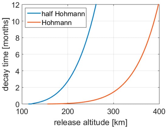
Figure 17.
Deorbiting with chemical propulsion, full Hohmann vs. half Hohmann, decay time vs. release altitude; 800 km initial altitude.
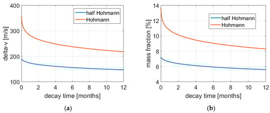
Figure 18.
Deorbiting with chemical propulsion, full Hohmann vs. half Hohmann, 800 km initial altitude: (a) delta-v; (b) propulsion system mass fraction.
In order to reduce this mass, it is possible to increase the altitude of the parking orbit, with the consequence of a longer total deorbiting time. However, as it can be seen in Figure 13 and Figure 14, the system mass has a low sensitivity to the total decay time, as the latter changes tremendously for a rather small variation in the final release altitude, thus not affecting much the propulsion system mass (the cases where the final and initial orbits are near, and where the propulsion system mass is small, are excluded).
As already pointed out earlier, a more efficient possibility is to simply decrease the perigee of the original orbit with a half Hohmann transfer up to a point where the decay time corresponds to the target one (Figure 15 and Figure 16). In this case, contrary to the circular orbit disposal, the decay time is not only dependent on the final (perigee) release altitude but also on the initial one (which remains the apogee altitude), as can be seen in Figure 15a.
Thanks to the exponential behavior of atmospheric density, the perigee of the new orbit is not much lower than the corresponding circular orbit (Figure 17). Consequently, the total delta-v and mass are only slightly higher than half the Hohmann transfer to the circular orbit (around 60%), guaranteeing a significant mass saving. The total mass is thus almost always below 10% of the satellite mass. The qualitative behavior remains the same as before, as it can be seen in Figure 18. The only advantage of the circular orbit disposal is that the satellite is immediately placed far outside the original orbit, while with the more efficient elliptic disposal, the apogee slowly descends from the initial altitude.
The mass model considered for this paper is very simplified. In reality the chemical propulsion system mass is a sublinear function of the propellant mass, particularly for small sizes and lower propellant masses. Thus, if a propulsion system is already onboard for other purposes like station keeping and/or orbit raising, the idea to use it also as a deorbiting device could guarantee important mass and cost benefits, together with the simplicity of having only a single system.
4.4. Electric Propulsion
Similarly to the chemical thruster, an electric thruster can also be used to lower the altitude up to a point where the aerodynamic drag will complete the deorbit. To do so for a fixed total time, it is necessary to increase the thrust of the electric propulsion system in order to speed up the active phase of the descent and let the natural decay do the rest of the deorbit in the remaining time. In this way, the delta-v is reduced and consequently some propellant is saved. However, this requires a larger thruster, and thus is heavier and more expensive. This situation is represented in Figure 19, Figure 20, Figure 21 and Figure 22.
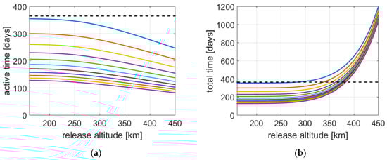
Figure 19.
Electric propulsion deorbiting with a combination of an active phase and a passive natural decay, parametric with thrust (0.5–1.5 mN): (a) active time vs. release altitude; (b) total time vs. release altitude. Black line is the one-year limit.
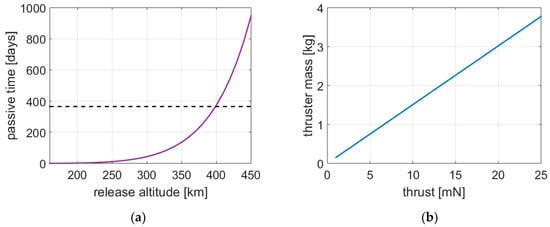
Figure 20.
Electric propulsion deorbiting with a combination of an active phase and a passive natural decay: (a) passive time vs. release altitude; (b) thruster mass vs. thrust.
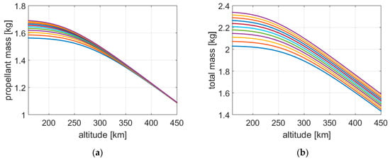
Figure 21.
Electric propulsion deorbiting with a combination of an active phase and a passive natural decay, with parametric thrust (0.5–1.5 mN): (a) propellant mass vs. release altitude; (b) total mass vs. release altitude.
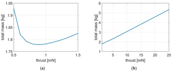
Figure 22.
Electric propulsion deorbiting with a combination of an active phase and a passive natural decay, total mass vs. thrust: (a) lower thrusts; (b) higher thrusts.
A satellite of 50 kg, with a density of 400 kg/m3, has been considered. The electric propulsion system has an Isp of 1000 s, α = 20 kg/kW, η = 0.65 and k = 0.25. The initial altitude is 850 km. The spacecraft is deorbited with the propulsion system up to a release altitude where it is left decaying naturally. The total deorbit time has been fixed in one year. The total time is the sum of the active phase and the passive decay. The passive decay is an exponential function of altitude, see Figure 20a. The release altitude should be less than 400 km in order to be compliant with the one-year limit. The active time is almost linear with the release altitude (Figure 19a), except at low altitudes where the drag force is comparable with the propulsion system thrust. The active time is almost linear with the thrust. The total time increases exponentially with the release altitude but intercepts the same limit at lower altitudes for lower thrusts.
The propellant mass follows the active time behavior with respect to the release altitude, and it is slightly dependent on thrust at low altitudes because of the increased aerodynamic drag savings at lower thrusts. The thruster mass is proportional to the thrust and consequently increases as the active decay time is reduced. The total mass of the propulsion system increases with the thrust and as the release altitude is decreased.
Once a specific total decay time is fixed (in this case one year), it is possible to plot the total mass of the propulsion system as a function of a single parameter, for example the thrust of the electric thruster. Higher thrusts mean shorter active descent time and the possibility to release the satellite at higher altitudes, saving propellant mass. However, as already seen with the chemical system, the exponential behavior of density and decay time with altitude gives a relatively low variation of the release altitude. Moreover, in this case, the total mass behavior seems dominated by the variation of the thruster mass with thrust (Figure 22b) even if a minimum of the curve is present (Figure 22a).
The results are dependent on the choices of thruster efficiency and specific impulse. Higher Isp and lower thruster efficiencies will exacerbate the optimization toward a minimum thrust solution. Higher initial altitudes will do the opposite. It is worth noting that larger thrusters, particularly at small scales, could provide much better performance in terms of Isp and efficiency. This non-linear effect could affect the optimization results toward a higher thrust solution. Technical limits in the total firing time could also have the same consequence.
For an electric propulsion system, it is also possible to activate the thruster only for a fraction of the orbit, around the apogee, in order to lower the perigee down to an altitude where the aerodynamic drag prevails and deorbits the spacecraft. This is analogous of the half Hohmann strategy for the chemical propulsion system, providing a propellant mass saving. However, in this case the deorbit is slow, and, for the same thrust, the decay time gets longer. In Figure 23, Figure 24, Figure 25 and Figure 26, an example is shown of an electric thruster that is activated in an arc of only 18° before and after the apogee, so 36° in total or 10% of the entire orbit.
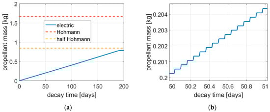
Figure 23.
Propellant mass consumption for an electric propulsion system that is activated only +/− 18° around the apogee: (a) full picture; (b) zoom in.
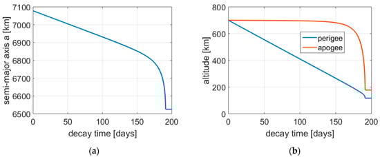
Figure 24.
Orbital decay for an electric propulsion system that is activated only +/− 18° around the apogee: (a) semi-major axis; (b) apogee and perigee.
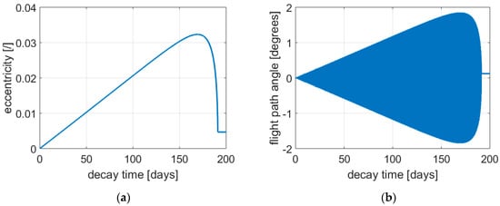
Figure 25.
Orbital decay for an electric propulsion system that is activated only +/− 18° around the apogee: (a) eccentricity; (b) flight-path angle.
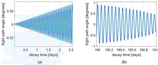
Figure 26.
Flight-path angle during orbital decay for an electric propulsion system that is activated only +/− 18° around the apogee: (a) initial perigee lowering; (b) drag circularization.
In Figure 23, it is possible to see the propellant consumption with time. In Figure 23b, it is possible to see that the thruster is activated only around 10% of the time. In Figure 23a, it is possible to see that the propellant mass linearly increases with time (albeit at steps) and reaches the value of the half Hohmann transfer strategy. The little discrepancy appears only at low release altitudes as the atmospheric drag adds on the propulsion thrust helping in a further propellant mass saving. In Figure 24 it is possible to see that this partial activation of the electric thruster reduces the energy of the orbit (i.e., its semi-major axis) mainly through a decrease in the perigee altitude. Only when atmospheric drag comes into play does circularization occur. The eccentricity of the orbit increases (remaining very small) with the flight-path angle (Figure 25) until drag-induced circularization occurs. Figure 26 shows two details of the increase in flight-path angle (i.e., eccentricity) forced by the apogee thrusting phases (Figure 26a) and of the final circularization induced by the atmospheric drag (Figure 26b).
It is interesting to see how this strategy works for a fixed decay time. In this case, the shortest is the activation time and the highest should be the thrust in order to complete the decay in the same time. Apparently, the thrust should be inversely proportional to the activation time. This is correct as an order of magnitude estimate, but it is necessary to consider that as the activation time is decreased, the energy required to be drawn from the orbit is also cut by almost half.
Consequently, if the thrust is scaled as the inverse of the activation time (Figure 27a), the decay time follows the behavior of Figure 27b. The decay time for short activation times is almost half the one for a continuous operation.
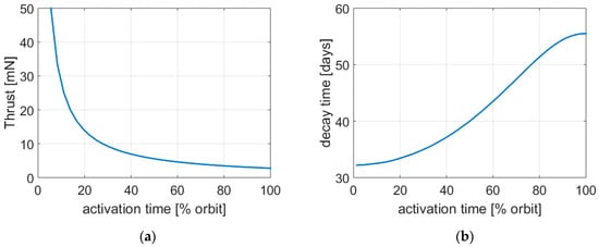
Figure 27.
Deorbiting with an electric propulsion system that is activated for a fraction of the orbit: (a) thrust; (b) decay time.
As expected, the total thruster actuation time is equal to the total decay time for continuous thrusting and goes to zero as the activation time fraction goes to zero (Figure 28a). This mean that partializing the activation time could help being compliant with thruster firing time limitations.
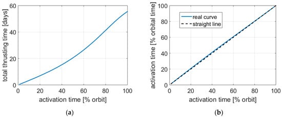
Figure 28.
Deorbiting with an electric propulsion system that is activated for a fraction of the orbit: (a) total thrusting time; (b) activation time vs. orbital fraction.
As the eccentricity is very low there is negligible difference between true anomaly, eccentric anomaly and mean anomaly; the same stands for activation time in terms of fraction of orbit or fraction of orbital period (Figure 28b).
The mass of the thruster is proportional to the thrust of the system, and so increases as the activation time is reduced (Figure 29a). The propellant mass shifts from the one of a half Hohmann maneuver to the one of a full Hohmann maneuver if the transfer does not reach very low altitudes. In the latter case, drag comes into, play further reducing the propellant mass need (Figure 29b).
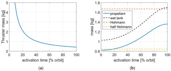
Figure 29.
Deorbiting with an electric propulsion system that is activated for a fraction of the orbit: (a) thruster mass; (b) propellant-related mass.
The effect of drag is much more prominent for continuous thrusting as all the orbit is spiraling down at low altitudes so the high drag can act along all the orbit and not only near the perigee.
The total mass of the system is the sum of the thruster mass and the propellant-related mass. The first is decreases with the activation time, while the other does the opposite. Comparing Figure 29 it is clear that it makes little sense to narrow too much the thrusting time near the apogee (let us say below 20%) as the propellant savings are little while the mass of the thruster soars.
In Figure 30 the total mass of the propulsion system has been calculated adjusting the thrust exactly to obtain the same total decay time (so something slightly different than Figure 27). Different decay times from 1 month to 12 months have been considered. It is possible to see that the total mass reduces as the decay time is increased because the thruster mass is reduced. Moreover, an optimum point is present at a specific activation time that minimizes the total mass as a compromise between propellant mass and thruster mass. The optimum point shifts toward the left as the decay time is increased because of the lower impact of the thruster mass. A continuous thrusting strategy is not that far from the optimum mass, particularly for short total decay times. The results depend on the selected thruster parameters: k = 0.25, Isp = 1000 s and η = 0.65. A lower thruster efficiency or a higher Isp will shift the optimal point toward a continuous firing strategy.
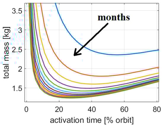
Figure 30.
Deorbiting with an electric propulsion system that is activated for a fraction of the orbit. Total mass as a function of activation time, and parametric with total deorbit time (1–12 months).
4.5. Electrodynamic Tether
The tether mass is linearly dependent on the (inverse) of the decay time. The tether mass is also dependent on the orbital inclination (trough the sine, squared) and proportional to the total displacement (i.e., distance between the original and final orbit). Its behavior is very similar to that of an electric thruster, but no propellant is consumed, so the best solution is always to use it continuously during all the descent phase in order to minimize the required drag force and consequently tether size and mass. The behavior of the tether will be better illustrated in the following comparison subsection.
4.6. Comparison
It is now interesting to compare the different behavior and performance of the various deorbiting technologies. Figure 31 shows the time profile of the altitude for the different technologies sized in order to have the same decay time. The initial orbit is circular, the initial altitude is 680 km and the decay time is one year for all cases.
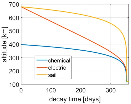
Figure 31.
Comparison of different deorbit technologies’ behavior, 680 km initial altitude. Orbital altitude with time.
The behavior of the electric thruster and the tether are the same if the thruster is fired continuously. Both systems induce a linear decrease in the orbital altitude until the drag prevails. The drag sail spends the majority of time near the initial altitude, and fall steeply near the end due to the atmospheric density profile with altitude. The chemical thruster immediately (compared with the total time) displaces the spacecraft to a new orbit at an altitude around 400 km to then fall slowly with the atmospheric drag in the same way the drag sail does at the higher altitude. This aspect is interesting to consider, as the decay altitude profile influences with time the way the system interacts with the other spacecrafts or debris. Even if the comparison is done for the same total decay time, there is a dramatic difference between spending almost one year in a crowded orbit or few hundred km below, for example.
A similar comparison can be also performed for an initial elliptical orbit. Again, comparing the deorbiting with a drag sail vs. a tether (or a continuously firing electric thruster), it is possible to recognize the different behavior. As the drag sail force is almost an exponential function of altitude, the decay is slower at the beginning and faster near the end. Moreover, the first phase is characterized by an orbit circularization, as the perigee (where the maximum force is applied) remains nearly constant while the apogee altitude decreases significantly. Near the end, the spacecraft spirals down. An increase of the drag sail area by a factor of ten causes a reduction of the deorbit time by the same amount (34 vs. 344 days in Figure 32a).
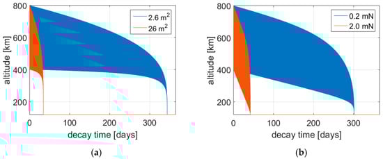
Figure 32.
Deorbiting behavior with different technologies and a tenfold increase in the drag force (a) drag sail; (b) tether.
For the tether, the force is almost the same for the entire orbit and during the whole decay. The resulting effect is an almost parallel linear decrease in both the perigee and apogee altitudes. When the perigee starts to be low, the satellite drag adds to the tether force and the circularization process begin. In this phase the perigee fall is still linear while the apogee one is more exponential. Finally, the spiraling down occurs. The nonlinear sum of the satellite drag with the tether force is more relevant when the two forces are comparable, i.e., at low altitudes and low tether forces. For this reason, a tenfold decrease in the tether thrust from 2 mN to 0.2 mN induces a sublinear increase of the decay time from 42 to 301 days (Figure 32b).
Regarding the performance aspect, it is interesting to compare the deorbiting time at different altitudes for a similar mass budget. In the following Figure 33, Figure 34 and Figure 35, a fixed mass budget of 4% has been imposed to the propellant-less systems, i.e., the sail and the tether, leaving the decay time to adjust consequently to the initial altitude. In the case of the electric thruster, the mass budget has been fixed equal to 4% mass for an initial altitude of 400 km (Figure 33). For higher altitudes the constant thruster mass has been kept the same and the propellant mass has been adapted to the higher delta-v, producing a slow variation (increase) of the total mass. The parameters for the electric propulsion are η = 0.65, k = 0.12 and Isp = 3000 s. For higher values of k and lower Isp the sensitivity of the total mass with the initial altitude increases. For the chemical propulsion system, the mass budget is mainly dependent on the propellant mass and thus the delta-v (k = 0.12, Isp = 300 s). As shown before, there is little room for the chemical system to trade mass for time. For this reason, the chemical propulsion mass is a strong function of the initial altitude.
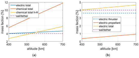
Figure 33.
Deorbiting with different technologies from LEO up to 150 km altitude, mass budget: (a) full picture; (b) zoom-in.
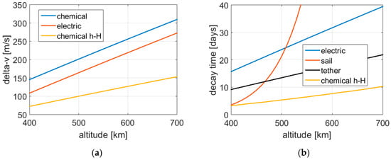
Figure 34.
Deorbiting with different technologies from LEO up to 150 km altitude: (a) delta-v; (b) decay time. Tether data calculated for 45° orbital inclination.
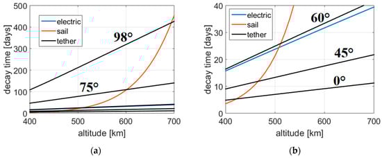
Figure 35.
Decay time vs. altitude for different technologies: (a) full picture; (b) zoom-in. Tether data are parametric with orbital inclination.
All the technologies consider a full deorbit down to 150 km. In case of the chemical propulsion system, both n Hohmann transfer to 150 km and a half Hohmann transfer to 150 km are considered for simplicity. The two are not exactly equivalent as shown before, as the first will provide immediate deorbit while the second should require a slightly lower perigee to be exact, otherwise the deorbit time is a bit longer but still negligible compared with the other technologies (Figure 34b).
The delta-v of the Hohmann and half Hohmann are plotted in Figure 34a as a function of the altitude together with the delta-v required by the electric propulsion system. The electric propulsion system is considered spiraling down through a continuous firing. For the reasons just explained, the delta-v of the half Hohmann is around 50% the full Hohmann (while it will be more correct to stay on a 60% value for the same decay).
The delta-v of the electric thruster is theoretically higher than the one of an impulsive full Hohmann transfer but, as stated earlier, at LEO altitudes the difference is negligible. However, as the descent with the electric thruster is slower, part of the delta-v is provided by the drag at the lowest altitudes (roughly the last 100 km, i.e., around 50 m/s), so the final result is the one plotted in Figure 34a and provides some propellant mass saving.
The decay times for the different technologies are shown in Figure 34b and Figure 35. It is possible to see that the chemical propulsion system is always the fastest but also generally the heaviest, except for small displacements, particularly with the half Hohmann strategy.
The drag sail is very efficient at low altitudes but becomes dramatically inefficient at higher altitudes due to the exponential behavior of atmospheric density.
As already pointed out earlier, the electric propulsion system and the tether have a similar behavior, with a slow, almost linear variation of decay time with initial altitude for the same mass budget. The tether is theoretically the best system in the majority of cases, except for high orbital inclinations where it becomes much less efficient than the electric thruster.
A similar analysis has also been performed at higher altitudes. In this case, instead of a full deorbit, it has been considered to reposition the spacecraft to a final circular orbit with a 5-year natural decay time (slightly below 500 km). The drag sail has been excluded from the analysis because at this altitude the repositioning time becomes unsustainable.
The results (Figure 36 and Figure 37) are analogous to the previous analysis. This time the delta-v of the full Hohmann transfer and the electric spiraling down are coincident, as the drag does not come into play at these altitudes (Figure 36a). For large displacements, the propellant mass budget of the chemical system grows to very high levels, and even the electric propulsion system is significantly affected.
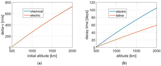
Figure 36.
Deorbiting with different technologies from high altitudes in LEO up to the altitude of a 5-year natural re-entry: (a) delta-v; (b) active descent time. Tether data calculated for 45° orbital inclination.
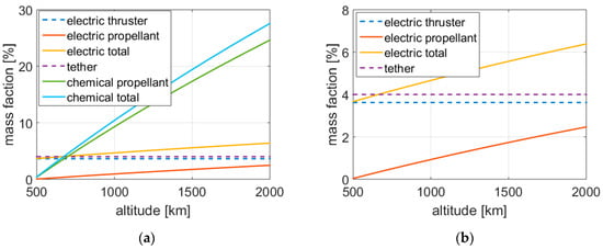
Figure 37.
Deorbiting with different technologies from high altitudes in LEO up to the altitude of a 5-year natural re-entry, mass budget: (a) full picture; (b) zoom-in.
The analysis has been repeated for a final natural decay time of 25 years. A 5-fold increase in the decay time provides only a few dozen km of higher final parking orbit altitude. For this reason, the results are almost equal to the previous ones (Figure 38 and Figure 39).
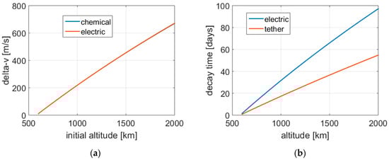
Figure 38.
Deorbiting with different technologies from high altitudes in LEO up to the altitude of a 25-year natural re-entry: (a) delta-v; (b) active descent time. Tether data calculated for 45° orbital inclination.
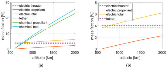
Figure 39.
Deorbiting with different technologies from high altitudes in LEO up to the altitude of a 25 years natural re-entry, mass budget: (a) full picture; (b) zoom-in.
This shows how there is little relative loss to significantly improve the decay time of a spent satellite, unless it is are already near the parking orbit (where the relative loss soars but the absolute effort vanishes). This suggests the opportunity to impose a tighter limit on new launched spacecrafts, as the long-term benefits of doing so seem to justify the relatively small added effort.
4.7. Combinations
It has been shown that the chemical system is fast but heavier, while the drag sail is simple and efficient at low altitudes. It is interesting to combine these two technologies, using the chemical system to rapidly move a spacecraft out from a crowded region and displace it at a lower altitude where the drag sail can perform more efficiently.
As an example, the deorbit from an 800 km initial circular orbit has been considered. A chemical propulsion system performs a Hohmann transfer from 800 km to a certain lower altitude called release altitude. The corresponding mass budget is calculated. Then, from the final parking orbit, a drag sail is sized in order to complete the deorbit in a certain prescribed amount of time. Three cases have been considered: 3 months, 12 months/1 year (×4) and 4 years (×4 again), together with two techniques for the chemical system, a full Hohmann transfer to the release altitude and a half Hohmann transfer that lowers only the perigee to the release altitude. The results are presented in Figure 40, Figure 41 and Figure 42.
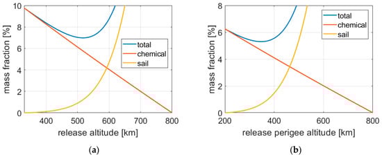
Figure 40.
Deorbiting with the serial combination of a chemical propulsion system and a drag sail, mass fraction vs. release altitude, 3-month total duration: (a) full Hohmann; (b) half Hohmann.
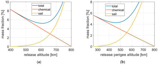
Figure 41.
Deorbiting with the serial combination of a chemical propulsion system and a drag sail, mass fraction vs. release altitude, 1-year total duration: (a) full Hohmann; (b) half Hohmann.
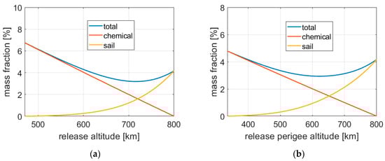
Figure 42.
Deorbiting with the serial combination of a chemical propulsion system and a drag sail, mass fraction vs. release altitude, 4-year total duration: (a) full Hohmann; (b) half Hohmann.
In all cases, the chemical propulsion system mass is zero if the release altitude is the initial altitude (i.e., the deorbiting is performed only by the drag sail) and grows linearly as the release altitude is reduced. On the contrary, the mass of the drag sail is zero if the maneuver is completed only by the chemical system down to the corresponding natural decay altitude and increases exponentially as the release altitude is lifted up.
The mass of the chemical system is dependent only on the release altitude while the mass of the drag sail is dependent on the inverse of the total decay time as less area is required. The sum of the two masses has a minimum for a certain release altitude. The minimum mass altitude shifts to the right if the decay time is increased as the required sail mass is decreased. For the same reason, the benefits of a combined solution compared to a propulsive-only solution increase as the decay time is extended. On the contrary the benefits of a combined solution compared to a sail-only solution vanish as the decay time is extended.
Obviously, the half Hohmann technique guarantees lower masses and shift the optimum toward the chemical propulsion side (left). The combination of a drag sail with a chemical propulsion system is surely more complex than a single solution but becomes particularly interesting if a propulsion system is already on board and the drag sail operate in a full passive and efficient mode (regarding attitude) after deployment.
Figure 43 shows the altitude behavior with time of an optimal combined solution vs. the two single-system solutions. As already shown earlier, the initial displacement by a chemical thruster is favorable to rapidly moving the spacecraft on a less crowded orbit (unless the opposite occurs, as could be in some cases). Moreover, the huge mass savings of the half Hohman technique are balanced by the drawback of sweeping continuously a wide range of different altitudes during the decay.
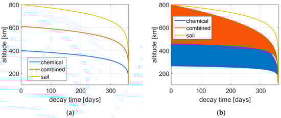
Figure 43.
Deorbiting with the serial combination of a chemical propulsion system and a drag sail, altitude with time, 1-year total duration: (a) full Hohmann; (b) half Hohmann.
Drag sails combined with tethers or electric thrusters are less attractive as the complexity starts to become relevant, and all three systems suffer from long decay times that will overlap in the mass budget.
A combination of a chemical system with a simple electrodynamic tether can be conceived in case a controlled re-entry is foreseen, but the total mass budget constraints do not allow for a full chemical solution.
A combination of an electric thruster with a tether could be conceived of for the following reasons:
- The tether in drag mode is able to generate power [40] that can be potentially used by the electric thruster;
- The two systems can potentially be integrated, sharing some components like the cathode and the power management system, thus providing a synergistic effect;
- A combined off-the-shelves system could be used at any orbital inclination with near-optimal performance. This is particularly interesting for constellations of satellites deployed in different orbital inclinations, where choosing a single combined commercial unit (instead of different ones, tether vs. electric, optimized for different inclinations) is advisable for mass production and integration.
4.8. Drag Compensation
A completely different approach to the deorbiting issue is to reverse the paradigm. Instead of taking care of deorbiting the spacecraft at the end of life, the satellite is placed directly at an altitude where the deorbiting is quick and assured by the natural aerodynamic decay. In this case, the propulsion system is not used to deorbit but to keep the satellite at the required altitude for its entire lifespan. This approach has important advantages. The first is the complete reliability of the deorbit process. While all the system previously discussed can fail preventing the proper deorbit of the spacecraft, in this case the deorbit is guaranteed. A failure of the propulsion system will lead to a failure of the mission and a premature re-entry of the spacecraft. From the standpoint of the space debris concern, this option is much more attractive.
It is interesting to compare the propellant mass required to keep a satellite at a certain altitude vs. the propellant mass required to deorbit the satellite. This is presented in the following Figure 44, Figure 45, Figure 46, Figure 47, Figure 48, Figure 49 and Figure 50.
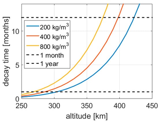
Figure 44.
Natural decay time for a 50 kg spacecraft, parametric with satellite density.
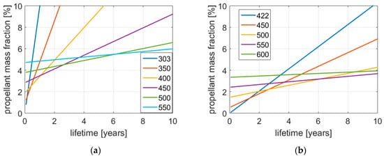
Figure 45.
Propellant mass fraction vs. lifetime for station keeping and deorbiting (from flight altitude) with a chemical thruster (Isp = 300 s, satellite mass 50 kg, density 200 kg/m3), parametric with flight altitude (km): (a) natural re-entry time of 1 month; (b) natural re-entry time of 1 year.
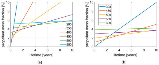
Figure 46.
Propellant mass fraction vs. lifetime for station keeping and deorbiting (from flight altitude) with a chemical thruster (Isp = 300 s, satellite mass 50 kg, density 400 kg/m3), parametric with flight altitude (km): (a) natural re-entry time of 1 month; (b) natural re-entry time of 1 year.
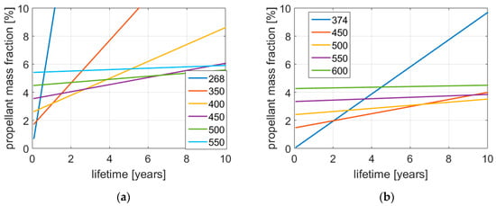
Figure 47.
Propellant mass fraction vs. lifetime for station keeping and deorbiting (from flight altitude) with a chemical thruster (Isp = 300 s, satellite mass 50 kg, density 800 kg/m3), parametric with flight altitude (km): (a) natural re-entry time of 1 month; (b) natural re-entry time of 1 year.
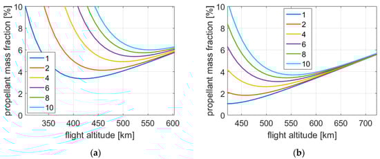
Figure 48.
Propellant mass fraction for station keeping and deorbiting (from flight altitude) with a chemical thruster (Isp = 300 s, satellite mass 50 kg, density 200 kg/m3), parametric with satellite lifetime (years): (a) natural re-entry time of 1 month; (b) natural re-entry time of 1 year.

Figure 49.
Propellant mass fraction for station keeping and deorbiting (from flight altitude) with a chemical thruster (Isp = 300 s, satellite mass 50 kg, density 400 kg/m3), parametric with satellite lifetime (years): (a) natural re-entry time of 1 month; (b) natural re-entry time of 1 year.
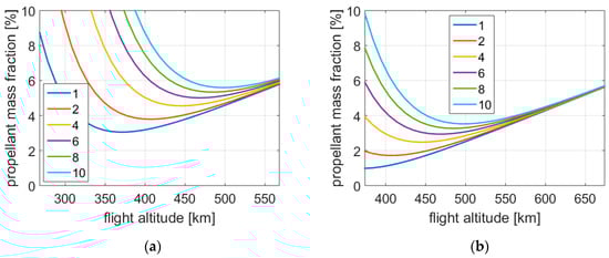
Figure 50.
Propellant mass fraction for station keeping and deorbiting (from flight altitude) with a chemical thruster (Isp = 300 s, satellite mass 50 kg, density 800 kg/m3), parametric with satellite lifetime (years): (a) natural re-entry time of 1 month; (b) natural re-entry time of 1 year.
Figure 44 shows the natural decay time of a spacecraft as a function of its initial altitude, parametric with the satellite density. The black lines correspond to the 1-month and 1-year limits. A higher ballistic coefficient allows a satellite to fly lower for the same decay time. From Figure 44, it is possible to infer the altitude required to naturally deorbit in 1 month (between 250 and 300 km) or 1 year (between 350 and 450 km).
The total propellant mass for the entire mission is the sum of the propellant mass for station keeping (i.e., drag compensation) at a certain altitude, plus the propellant mass required for repositioning at the altitude of the 1-month or 1-year limit. The propellant mass for drag compensation is linear with the satellite lifetime and (inversely) exponential with the flying altitude. Conversely, the propellant mass for deorbiting is independent from the satellite lifetime and almost linearly increases with the flying altitude. The resulting total propellant mass is a straight line that starts at a certain level (deorbiting needs) that is higher as the flying altitude increases. The slope of the straight line is related to the propellant mass consumed for station keeping. The lower the altitude, the higher the slope of the straight line because of the increased drag. The final pattern is visible in Figure 45, Figure 46 and Figure 47. The difference between the left figures and the right figures is the final altitude, which corresponds to the 1-month and 1-year limit, respectively. The difference between the three figures (Figure 45, Figure 46 and Figure 47) is the satellite density (i.e., ballistic coefficient).
The qualitative results are the same for all figures. Satellites flying at low altitude have a small deorbit need, but the propellant mass rapidly increases with satellite lifetime. On the contrary, spacecraft flying at higher altitudes have a significant deorbit need but the propellant mass varies little with the satellite lifetime as drag compensation requires little delta-v at those altitudes. Thus, short lifetimes favor low-flying satellites, while the opposite occurs for long lifetimes. Higher ballistic coefficients shift the optimal orbit to lower altitudes. Longer final decay times provide a higher minimum altitude and lower deorbit propellant mass needs.
Another way to present the results is shown in Figure 48, Figure 49 and Figure 50. The same cases have been considered. This time the propellant mass fraction is presented as a function of the flying altitude, parametric with the satellite lifetime. It is possible to see that an optimal altitude exists that minimizes the total propellant consumption. Above the optimal altitude, increased deorbiting needs cause a higher propellant mass, while below, drag compensation is to be blamed.
The optimal altitude shifts to the right as the lifetime is extended because of the total impulse increase for drag compensation. The curves shift to the left as the ballistic coefficient is improved. As expected from the results highlighted in the previous figures, the results have very low sensitivity to the lifetime on the right of the graphs, where deorbiting need prevails, and a very high sensitivity on the left, where drag compensation prevails. Consequently, the optimal points for shorter lifetimes perform poorly for longer lifetimes, while the optimal points for longer lifetimes are not as bad for short lifetimes.
Finally, the effects of a different re-entry time limit (in this case 1 month vs. 1 year) are only to decrease the propellant mass requirements and set a higher minimum altitude threshold, but the curves’ behavior seems the same with the same optimal altitudes.
Electric propulsion is particularly suited for drag compensation as the thrust (thus power) requirements are relatively low (without the thrust/time trade-off of deorbiting) and the high specific impulse limits the propellant mass burden [50].
It is important to highlight that flying at lower altitudes can have important side benefits other than the deorbiting aspects, particularly for Earth observation missions. In reality, these advantages are much more than simple side benefits, and they can already justify the choice of a lower-than-usual flying altitude by their own [51].
5. Other Topics
There are some other aspects that are interesting to be outlined in the framework of this paper, and they will be presented in this chapter.
5.1. Integrated vs. Independent System
The deorbiting device can be conceived of as an integrated or an independent subsystem of the spacecraft. In the first case, the satellite provides all the basic functions like attitude determination and control, communication, power and so on. This is the most common situation and provides generally the simplest, cheapest and lightweight solution. However, this option requires the satellite to stay alive and working up to the end of the mission, maybe not completely functional regarding the payload or other non-strictly necessary capabilities, but still capable of operating the deorbit correctly.
Approximately, the probability of the satellite to perform a successful re-entry is the product of the reliability of the deorbiting device/maneuver multiplied by the probability of the satellite to survive up to the end of the deorbit, which, as expected in general, in case the active part of the deorbiting is short compared to satellite lifetime, it is mainly related with the satellite surviving up to the decommissioning date. Some solutions can be considered inherently more reliable, for example a chemical propulsion system provides a short and thus less risky deorbit compared with a tether or an electric thruster, and a passive drag sail will also have a short active phase. For the reasons just highlighted, if the satellite has an average predicted lifetime with a certain uncertainty, it is necessary to end the mission and deorbit the satellite prematurely if a high success rate is sought, based on statistical analysis. The higher the lifetime uncertainty and the target success rate, the shorter will be the mandatory decommissioning time limit compared with the real average satellite lifetime.
One possible means to improve the effectiveness of this solution is to exploit the live monitoring and prediction of the satellite health. Thanks to modern artificial intelligence (AI) capabilities, it will be likely possible in the future to better assess the probability of failure of a specific spacecraft based on the story of its own health data compared with other similar assets. This could be particularly effective for large constellations of equal satellites.
In the opposite direction, an alternative solution is to equip the satellite with a fully autonomous deorbiting device that can be activated and operated successfully independently from the satellite, giving the possibility to wait until the satellite is dead. This could be particularly interesting for large systems with very long lifetimes that make huge profits for every (relatively small but absolutely massive) increase in operational time, and thus do not want to be prematurely decommissioned. This kind of system has been proposed, for example, by D-Orbit [52]. The issues of this solution are mainly two. The first drawback is the duplication of several satellite functions, which will bring added costs and weight. This is particularly true for small platforms, while probably much less of a deal for larger ones (D-Orbit claims an added mass of few percent for a large GEO telecom sat). The second, very demanding challenge, is to fully guarantee the deorbit of a non-functional satellite in all (or almost all) the situations, particularly regarding damaged and or uncontrolled systems that have lost their attitude and are tumbling.
It is also possible that for some type of deorbiting devices a sort of intermediate solution is possible, where the main satellite can lose a significant but not complete part of its functions and still deorbit safely.
5.2. Active Debris Removal and Life Extension
While the bulk of the paper deals with the autonomous re-entry of a spacecraft and focuses on future objects launched into space, it is important to remember that there is a high chance that there will be the need to retrieve large objects already in space, particularly part of spent upper stages. To do that is necessary to perform an active debris removal (ADR) mission [36,37,53].
Active debris removal is by far more complex than the simple deorbiting of a satellite because the chasing spacecraft has to reach the target, approach it, grab it and to bring it back to the edge of the atmosphere or on a disposal orbit. The analysis of all these problematics is out of the scope of this paper and the reader is referred to the corresponding appropriate literature. What is worth mentioning here is that the propulsion/deorbiting systems should have several analogies with the one described previously, but with more demanding delta-v and functional requirements as the chasing spacecraft has to move first toward the target, doing proximity operations and deorbit it afterwards, sometimes capturing and deorbiting more than one object in the same mission. The technical advantage of an ADR platform is that the total lifetime of this system can be much shorter than that of a typical satellite, simplifying some engineering aspects. This is particularly true in case the target is a medium/large platform with a long lifetime.
ADR platforms could also highly benefit by strong synergies from future development in the so called in-orbit servicing market and in all the applications that require some sort of space tug. Another interesting related application is life extension, where the satellite lifetime is extended by the arrival of some kind of servicing platform.
It is also possible that future regulations will force ADR for satellites that have failed to deorbit. If the servicing market will achieve great success, it is even possible that the original satellites will not be equipped with a deorbiting device and then simply captured and disposed after death, booking the service (maybe in advance) from a commercial provider.
5.3. Type of Re-Entry
The re-entry of a spacecraft can be controlled or uncontrolled. In the latter, the system is deorbited without consideration on the actual re-entry corridor on the atmosphere. The uncontrolled re-entry simplifies the system design, and all the possible deorbiting devices, can be used, active or passive, fast or slow. On the contrary, for a controlled re-entry, it is necessary to have a system package that is able to direct the spacecraft toward a specific region of Earth.
Uncertainties in the orbit and attitude prediction are dominated by the large uncertainties in the atmospheric model, and in the solar and geomagnetic activity forecasts. For this reason, the final re-entry corridor can be predicted accurately only near the final orbit and thus controlled re-entry requires a quick and steep descent from a region of relatively thin density (where the satellite is easy to control) through the higher density layers of the atmosphere (where aerodynamic force and torque disturbances are dominant). Consequently controlled re-entry requires generally a chemical propulsion system, or a drag sail deployed at the right time at very low altitude (but not at high altitude, unless the area can be actively adjusted). Such a controlled re-entry under a relatively steep atmospheric incidence angle produces a confined ground impact area of break-up fragments which have survived the aerothermal heating. The ground impact area must be selected such that a tolerable residual risk to persons on ground can be achieved.
Controlled re-entry is mandatory for recoverable and/or reusable systems, which are rare at present but seem go be becoming more frequent in the next future, even for small platforms. In these cases, re-entry accuracy is even more important in order to allow safe landing and recover. Controlled re-entry is also necessary for expendable spacecrafts that produce particularly large and/or dangerous debris. NASA re-entry requirements [10] dictate the risk of human casualty anywhere on Earth due to a reentering debris with Kinetic Energy KE ≥ 15 J be less than 1:10,000 (0.0001). This applies especially for denser materials, thicker structures, and more protected components.
An alternative possibility is design for demise [53,54,55,56,57]. In this case the expendable satellite is designed to burn completely in the atmosphere. Demisable designs will tend to favor lighter materials, thinner structures, and more exposed components. Design for demise allows the simplicity, reliability and multiple choice in deorbiting solutions of uncontrolled re-entry. However, design for demise requirements can partially conflict with design for survivability in space ones.
6. Conclusions
LEO satellite population is expected to grow dramatically in the coming years. To avoid a corresponding unacceptable increase in the rate of collision with debris or collision avoidance operations it is necessary to keep the LEO region clean. The current 25 year-limit, which corresponds to a natural decay from around 600 km, will become probably insufficient in the future and faster ways to deorbit are to be sought.
This paper focused the attention on the means for effectively deorbiting a spacecraft. Four technologies for deorbiting have been investigated: drag sail, chemical propulsion, electric propulsion, electrodynamic tether. Both simplified numerical models and full integration of the dynamic equations with a 4th order Runge–Kutta scheme have been used in order to compare the deorbit behavior of the different technologies and highlight their impact at system level.
Solar sails have been excluded from deep analysis as they have been shown to be inefficient for deorbiting, as the force they produce from about 4.5 μN/m2 solar pressure is by far inferior to competing technologies, except maybe for drag sails at higher altitudes. In addition, they need to be controlled on each orbit for a very long time.
Drag sails are very effective at low altitude and long decay times, and they can be passive after deployment. Sail mass is almost inversely linear with decay time. However, they become inefficient and too slow at higher altitudes. With a relative mass between 1 and 4% of the satellite, they can deorbit a satellite in less than 5 years up to 700–800 km, and less than 25 years up to 800–1000 km.
Chemical propulsion allows for fast and controlled deorbit from any altitude but tends to be the heavier option if the time constraint is relaxed as this technology has limited sensitivity to deorbit time. Re-entry times of less than an hour can be achieved with a system mass fraction up to 20% at 1200 km.
Chemical propulsion can deorbit the satellite with a Hohmann transfer to a lower altitude or can lower its perigee with a half Hohmann maneuver. The second option allows for nearly 40% propellant savings but keeps the satellite orbiting in a wide range of altitudes unless the perigee is already sufficient for direct re-entry.
Electric propulsion can provide important mass savings compared with the chemical option, particularly for high delta-v (i.e., higher altitudes), thanks to its superior specific impulse. Delta-v losses for continuous firing have been shown to be negligible in LEO. However, the power (thrust) constraint forces a slower process, in the order of months. With mass fractions comparable to a drag sail, an electric propulsion system can provide much shorter deorbit times at higher altitudes, approximately starting from above 500 km altitude. For a fixed specific impulse, the electric propulsion system mass decreases asymptotically with the deorbit time down to the bare propellant tank wet mass.
The electric thruster can be fired continuously in order to provide a spiral decay of the orbit or operated only near the apogee to lower the perigee. The second option provides significant propellant mass savings at the expense of longer operating times or higher thruster size (i.e., mass and cost). Near-continuous firing guarantees the minimum total mass for short deorbit times (few months) at high specific impulses while lower duty cycles have a potential for up to 40% mass savings for long decay times (several months) at lower specific impulses. Duty cycles below 20% provide no benefits.
Electrodynamic tethers have the potential to be the most lightweight solution, especially for long decay time as their mass is inversely linear to decay time, with the exception of high orbital inclinations where they suffer from poor performance due to the alignment with the magnetic field. In fact, for the same mass budget, induced drag forces can be up to 2–3 times the one from a corresponding electric thruster for inclination up to 45°. Above around 60° parity is achieved, while near a polar orbit the thrust drops to near zero. They are also the less mature technology for the moment.
The most interesting combination is chemical propulsion with a drag sail, which are the most different between each other but both relatively simple. In fact, the first is fast and effective at any altitude (included higher ones) but becomes heavy for large displacements, while the second is slow but passive, lightweight and much more effective at low altitudes. A proper combination of the two technologies can provide a minimum mass solution that rapidly take out the spacecraft from the original (crowded) orbit and let it decay slowly from a lower altitude. For very short times the total mass approaches the one of a chemical-only system, while for very long times the total mass approaches the one of a sail-only system. For intermediate deorbit times on the order of 1 year savings around 30% are potentially possible.
The deorbit device can be integrated or independent. The first solution is generally the simplest, cheapest and lightweight but requires the satellite to stay alive up to disposal. An independent system is more challenging (and probably heavier and expensive in total) but could provide deorbit after satellite death, giving the possibility to exploit the full satellite lifetime. This is particularly interesting for large platforms with very long lifetimes. Health monitoring can help the integrated solution to adapt to the single satellite history.
Active debris removal is a possibly interesting future option both to retrieve current space junk but also for new spacecrafts that fail to deorbit or that do not carry a disposal system. This technology could go hand in hand with life extension solutions and the general new paradigm of commercial in-orbit servicing.
Re-entry can be controlled or uncontrolled. The first solution requires a high thrust solution, at least for the terminal part, and it is necessary for recoverable/reusable systems or spacecrafts that produce dangerous debris upon re-entry. The uncontrolled re-entry is a simpler and more flexible option but requires compliance with design for demise practices.
A completely different paradigm is drag compensation. In this casem no deorbit device is necessary and re-entry is guaranteed at the end of life as the satellite flies at very low altitudes. This solution requires a propulsion system for station keeping. Drag compensation is favored by shorter lifetimes (few years), higher specific impulses (e.g., electric propulsion) and high ballistic coefficients (i.e., slender design) and is particularly interesting for Earth observation missions where a lower altitude can improve the resolution by a factor of 2.
Plenty of options are available for deorbiting satellites in LEO, and this paper can be used as a starting point for mission/system design, trade-offs and preliminary selection.
The most important step forward currently seems to be the regulatory framework, imposing stricter rules and active mandatory sanctions.
Funding
This research received no external funding.
Institutional Review Board Statement
Not applicable.
Informed Consent Statement
Not applicable.
Data Availability Statement
Not applicable.
Acknowledgments
The author wants to thank Giulia Sarego (now at Technology for Propulsion and Innovation, T4i) for helping with the reference material. A thank you also to Daniele Pavarin (University of Padova and T4i CEO) for useful ideas.
Conflicts of Interest
The author declares no conflict of interest.
References
- Space.com. Available online: https://www.space.com/spacex-starlink-satellite-collision-alerts-on-the-rise (accessed on 19 August 2022).
- Parabolic Arc. Available online: http://parabolicarc.com/2022/07/17/swarm-dodges-collision-during-climb-to-escape-suns-wrath/#more-87593 (accessed on 19 August 2022).
- Ars Technica. Available online: https://arstechnica.com/information-technology/2017/10/spacex-and-oneweb-broadband-satellites-raise-fears-about-space-debris/ (accessed on 19 August 2022).
- Parabolic Arc. Available online: http://parabolicarc.com/2022/03/26/space-situational-assessment-2021-the-growing-menace-of-space-debris/ (accessed on 19 August 2022).
- Kessler, D.J.; Cour-Palais, B.G. Collision frequency of artificial satellites: The creation of a debris belt. J. Geophys. Res. Space Phys. 1978, 83, 2637–2646. [Google Scholar] [CrossRef]
- Karacalioglu, A.G.; Stupl, J. The Impact of New Trends in Satellite Launches on the Orbital Debris Environment. In Proceedings of the NASA: 8th IAASS Conference, Safety first, Safety for All, Melbourne, FL, USA, 18–20 May 2016. [Google Scholar]
- ESA Space Debris Office. ESA’s Annual Space Environment Report; GEN-DB-LOG-00288-OPS-SD; ESA: Darmstadt, Germany, 2020. [Google Scholar]
- Wittig, M. Space Debris and De-Orbiting. MEW Aerospace. In TU Symposium and Workshop on Small Satellite Regulation and Communication Systems; Czech Republic: Prague, Czech, 2–4 March 2015. [Google Scholar]
- SpaceX. Available online: https://www.spacex.com/rideshare/ (accessed on 19 August 2022).
- ESA. Available online: https://www.esa.int/Enabling_Support/Operations/Space_debris_mitigation_the_case_for_a_code_of_conduct (accessed on 19 August 2022).
- Hull, S.M. NASA Disposal Guidelines. 2013. Available online: https://ntrs.nasa.gov/citations/20130000278 (accessed on 19 August 2022).
- IADC Steering Group and Working Group 4. IADC Space Debris Mitigation Guidelines. 2020. Available online: https://www.google.com/url?sa=t&rct=j&q=&esrc=s&source=web&cd=&ved=2ahUKEwjzwbyA7df6AhUL3KQKHQgHDDsQFnoECAwQAQ&url=https%3A%2F%2Fwww.iadc-home.org%2Fdocuments_public%2Ffile_down%2Fid%2F5249&usg=AOvVaw3Y9m5766xNnRyXuPdNPtW5 (accessed on 19 August 2022).
- Parabolic Arc. Available online: http://parabolicarc.com/2022/02/24/spacexs-approach-to-space-sustainability-and-safety/ (accessed on 19 August 2022).
- Parabolic Arc. Available online: http://www.parabolicarc.com/2022/07/20/neuraspace-creates-smart-traffic-management-solution-for-satellite-constellations/ (accessed on 19 August 2022).
- Janovsky, R. End-Of-Life De-Orbiting Strategies for Satellites. In Proceedings of the 54th International Astronautical Congress of the International Astronautical Federation, the International Academy of Astronautics, and the International Institute of Space Law, Bremen, Germany, 29 September–3 October 2003. [Google Scholar] [CrossRef]
- Cornara, S.; Beech, T.; Belló-Mora, M.; Martinez de Aragon, A. Satellite Constellation Launch, Deployment, Replacement, and End-Of-Life Strategies. SSC99-X-1. In Proceedings of the 13th Annual AIAA/USU Conference on Small Satellites, Logan, Utah, 23–26 August 1999. [Google Scholar]
- Sanchez-Arriaga, G.; Sanmartin, J.R.; Lorenzini, E.C. Comparison of technologies for deorbiting spacecraft from low-earth-orbit at end of mission. Acta Astronaut. 2017, 138, 536–542. [Google Scholar] [CrossRef]
- Steyn, W.H. De-Orbiting Strategies; Stellenbosch University: Stellenbosch, South Africa.
- Mostafa, A.; El-Saftawy, M.I.; Abouelmagd, E.I.; López, M.A. Controlling the perturbations of solar radiation pressure on the Lorentz spacecraft. Symmetry 2020, 12, 1423. [Google Scholar] [CrossRef]
- Abouelmagd, E.I.; Mortari, D.; Selim, H.H. Analytical study of periodic solutions on perturbed equatorial two-body problem. Int. J. Bifurc. Chaos 2015, 25, 1540040. [Google Scholar] [CrossRef]
- Abouelmagd, E.I. Periodic solution of the two–body problem by KB averaging method within frame of the modified Newtonian potential. J. Astronaut. Sci. 2018, 65, 291–306. [Google Scholar] [CrossRef]
- U.S. Standard Atmosphere; U.S. Government Printing Office: Washington, DC, USA, 1976.
- Picone, J.M.; Hedin, A.E.; Drob, D.P.; Aikin, A.C. NRLMSISE-00 empirical model of the atmosphere: Statistical comparisons and scientific issues. J. Geophys. Res. Space Phys. 2002, 107, 1468. [Google Scholar] [CrossRef]
- Parabolic Arc. Available online: http://parabolicarc.com/2022/06/14/space-flight-laboratory-announces-successful-deorbiting-of-nanosatellite-with-drag-sail-technology/ (accessed on 19 August 2022).
- Black, A.; Spencer, D.A. DragSail systems for satellite deorbit and targeted reentry. J. Space Saf. Eng. 2020, 7, 397–403. [Google Scholar] [CrossRef]
- Long, A.C.; Spencer, D.A. A Scalable Drag Sail for the Deorbit of Small Satellites. J. Small Satell. 2018, 7, 773–788. [Google Scholar]
- Taylor, B.; Fellowes, S.; Dyer, B.; Viquerat, A.; Aglietti, G. A modular drag-deorbiting sail for large satellites in low Earth orbit. In Proceedings of the SciTech 2020, Orlando, FL, USA, 6–10 January 2020. [Google Scholar]
- Sikes, J.D.; Ledbetter, W.; Sood, R.; Medina, K.; Turse, D. Keeping Low Earth Orbit Clean: Deorbit Analysis for an Articulating Boom Drag Sail. Adv. Astronaut. Sci. 2020, 175, 1–15. [Google Scholar]
- Faber, D.; Overlack, A.; Welland, W.; van Vliet, L.; Wieling, W.; Tata Nardini, F. Nanosatellite deorbit motor. SSC13-I-9. In Proceedings of the 27th annual AIAA/USU Conference on Small Satellite, Logan, Utah, 12–15 August 2013. [Google Scholar]
- Schonenborg, R.A.C.; Schöyer, H.F.R. Solid Propulsion De-Orbiting and Re-Orbiting. In Proceedings of the 5th European Conference on Space Debris, Darmstadt, Germany, 30 March–2 April 2009. [Google Scholar]
- Schonenborg, R.A.C. Solid propellant de-orbiting for constellation satellites. In Proceedings of the 4th International Spacecraft Propulsion Conference, Chia Laguna, Italy, 2–9 June 2004. [Google Scholar]
- Barato, F. Challenges of Ablatively Cooled Hybrid Rockets for Satellites or Upper Stages. Aerospace 2021, 8, 190. [Google Scholar] [CrossRef]
- Barato, F.; Paccagnella, E.; Pavarin, D. Explicit Analytical Equations for Single Port Hybrid Rocket Combustion Chamber Sizing. J. Propuls. Power 2020, 36, 869–886. [Google Scholar] [CrossRef]
- Barato, F.; Bellomo, N.; Pavarin, D. Integrated approach for hybrid rocket technology development. Acta Astronaut. 2016, 128, 257–261. [Google Scholar] [CrossRef]
- Barato, F.; Grosse, M.; Bettella, A. Hybrid Rocket Residuals—An Overlooked Topic. AIAA 2014-3753. In Proceedings of the 50th AIAA/ASME/SAE/ASEE Joint Propulsion Conference & Exhibit, Cleveland, OH, USA, 28–30 July 2014. [Google Scholar] [CrossRef]
- Tadini, P. Hybrid Rocket Propulsion for Active Removal of Large Abandoned Objects. Ph.D. Thesis, Politecnico di Milano, Milan, Italy, 2014. [Google Scholar]
- Tonetti, S.; Cornara, S.; Faenza, M.; Verberne, O.; Langener, T. Feasibility Study of Active Debris Removal Using Hybrid Propulsion Solutions. In Proceedings of the Stardust Global Virtual Workshop II, Southampton, UK, 19–22 January 2016. [Google Scholar]
- MIT OpenCourseWare 16.522 Space Propulsion; Springer: Cambridge, MA, USA, 2015; Available online: http://ocw.mit.edu (accessed on 19 August 2022).
- Sarego, G.; Olivieri, L.; Valmorbida, A.; Bettanini, C.; Colombatti, G.; Pertile, M.; Lorenzini, E.C. Deorbiting Performance of Electrodynamic Tethers to Mitigate Space Debris. World Academy of Science, Engineering and Technology. Int. J. Aerosp. Mech. Eng. 2021, 15, 185–191. [Google Scholar]
- Bilen, S.; McTernan, J.; Gilchrist, B.; Bell, I.; Voronka, N.; Hoyt, R. Electrodynamic Tethers for Energy Harvesting and Propulsion on Space Platforms. AIAA 2010-8844. In Proceedings of the AIAA SPACE 2010 Conference & Exposition, Anaheim, CA, USA, 30 August–2 September 2010. [Google Scholar]
- Olivieri, L.; Mantellato, R.; Francesconi, A. A Tethered Space Tug Concept Demonstration for Active Debris Removal Missions. In Proceedings of the ESA GNC 2017, Salzburg, Austria, 29 May–June 2017. [Google Scholar]
- Thethers Unlimited CubeSat Terminator Tape Brochure. Available online: https://www.tethers.com/ (accessed on 19 August 2022).
- Thethers Unlimited NanoSat Terminator Tape Brochure. Available online: https://www.tethers.com/ (accessed on 19 August 2022).
- Aurora Propulsion Technologies APB-S Brochure. Available online: https://www.aurorapt.fi (accessed on 19 August 2022).
- Montenbruck, O.; Gill, E. Satellite Orbits: Models, Methods and Applications; Springer: Berlin, Heidelberg, 2001. [Google Scholar] [CrossRef]
- Chobotov, V.A. Orbital Mechanics, 3rd ed.; AIAA Education Series; American Institute of Aeronautics and Astronautics, Inc.: Reston, VA, USA, 2008. [Google Scholar]
- Vallado, D.A. Fundamental of Astrodynamics and Applications, 2nd ed.; Microcosm Press: El Segundo, CA, USA; Kluwer Academic Publishers: Boston, MA, USA, 2001. [Google Scholar]
- GOCE ESA’s Gravity Mission. Available online: https://www.esa.int/Applications/Observing_the_Earth/FutureEO/GOCE (accessed on 19 August 2022).
- Klinkrad, H.; Sanchez-Ortiz, N. Collision Avoidance for Operational ESA Satellites. ESA SP-587. In Proceedings of the 4th European Conference on Space Debris, Darmstadt, Germany, 18–20 April 2005. [Google Scholar]
- Barato, F.; Trezzolani, F.; Manente, M.; Pavarin, D.; Andreussi, T.; Andrenucci, M. Electric Propulsion Technology for Low Earth Mission of Micro/Nano-Satellites. In Proceedings of the International Astronautic Conference 2015, Jerusalem, Israel, 12–16 October 2015. [Google Scholar]
- Bertolucci, G.; Barato, F.; Toson, E.; Pavarin, D. Impact of propulsion system characteristics on the potential for cost reduction of earth observation missions at very low altitudes. Acta Astronaut. 2020, 176, 173–191. [Google Scholar] [CrossRef]
- Rossettini, L. Technical Day on “Deorbiting Strategies”. Available online: https://www.dorbit.space/ (accessed on 1 December 2015).
- Innocenti, L. Clean Space; ESA Clean Space Office: Darmstadt, Germany, 2019. [Google Scholar]
- Astromaterials Research & Exploration Science NASA Orbital Debris Program Office. Available online: https://orbitaldebris.jsc.nasa.gov/reentry/ (accessed on 19 August 2022).
- Eggen, N.; Tiago Soares, T.; Innocenti, L. Containment Methods for The Atmospheric Reentry of Satellites. In Proceedings of the First Int’l. Orbital Debris Conference, Sugar Land, TX, USA, 9–12 December 2019. [Google Scholar]
- Trisolini, M.; Lewis, H.G.; Colombo, C. On the Demisability and Survivability of Modern Spacecraft. In Proceedings of the 7th European Conference on Space Debris, Darmstadt, Germany, 18–21 April 2017; Flohrer, T., Schmitz, F., Eds.; The ESA Space Debris Office: Darmstadt, Germany, 2017. Available online: http://spacedebris2017.sdo.esoc.esa.int (accessed on 1 June 2017).
- Waswa, M.B.P. Spacecraft Design-for-Demise Strategy, Analysis and Impact on Low Earth Orbit Space Missions. Master’s Thesis, Massachusetts Institute of Technology, Cambridge, MA, USA, 2009. [Google Scholar]
Publisher’s Note: MDPI stays neutral with regard to jurisdictional claims in published maps and institutional affiliations. |
© 2022 by the author. Licensee MDPI, Basel, Switzerland. This article is an open access article distributed under the terms and conditions of the Creative Commons Attribution (CC BY) license (https://creativecommons.org/licenses/by/4.0/).