
Geometric Nonlinear Analysis of the Catenary Cable Element Based on UPFs of ANSYS


Abstract
:1. Introduction
2. Tangential Stiffness Matrix of Two-Node Catenary Cable Element Based on UL Formulation
2.1. Basic Assumptions
- The stress-strain relationship of the cable conforms to Hooke’s law.
- The cable cannot be subjected to compression and bending but only to tension, being ideally flexible.
- The cross-section of the cable does not change under external loading.
- The self-weight constant load set of the cable is consistent along the length of the cable.
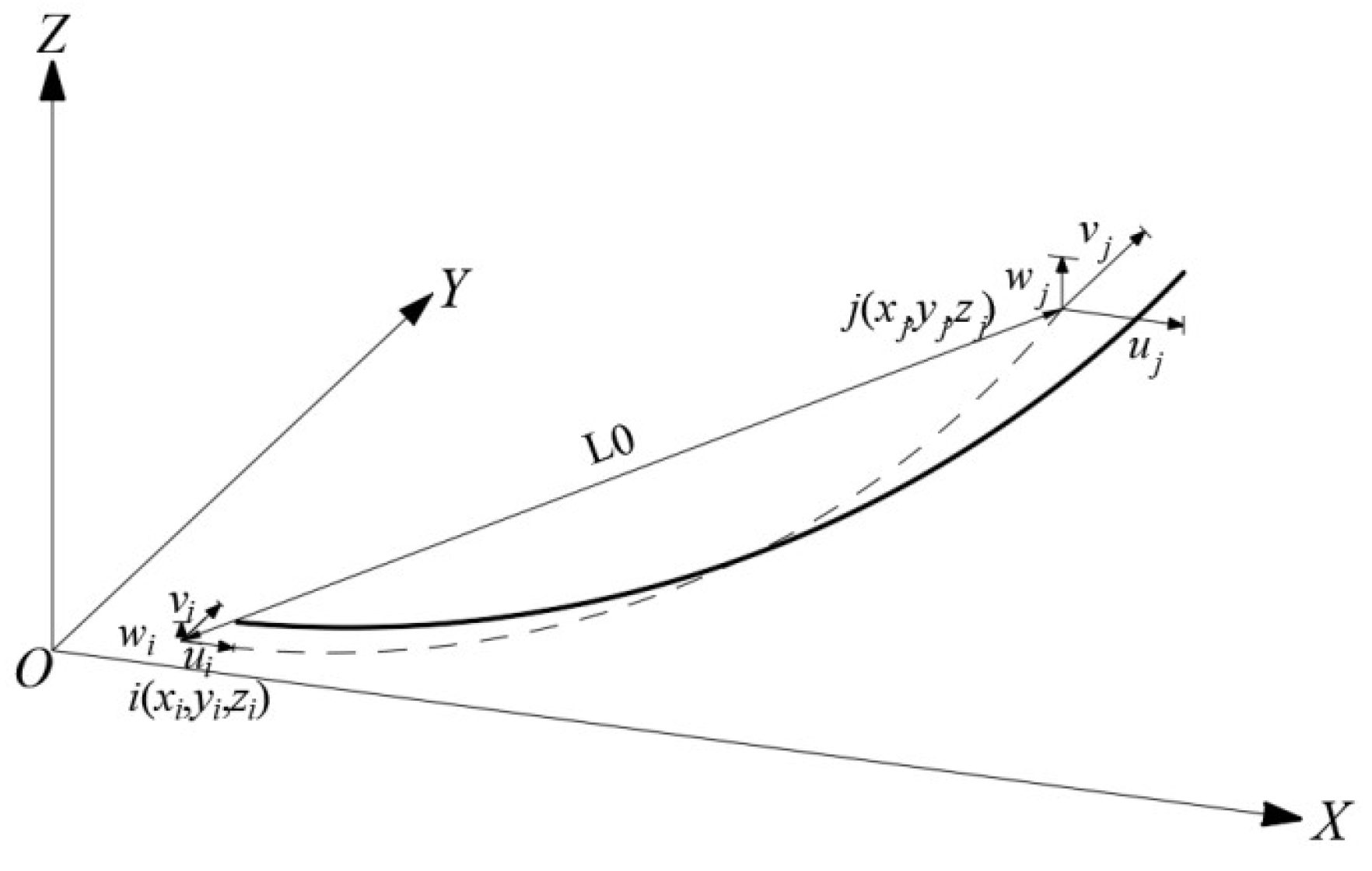
2.2. Tangential Stiffness Matrix of the Catenary Cable Element
2.3. Iterative Solution of a Catenary Cable Element with Known Pretension Tj or Ti
2.4. Iterative Solution of the Tangential Stiffness Matrix of a Catenary Cable Element with Known S0
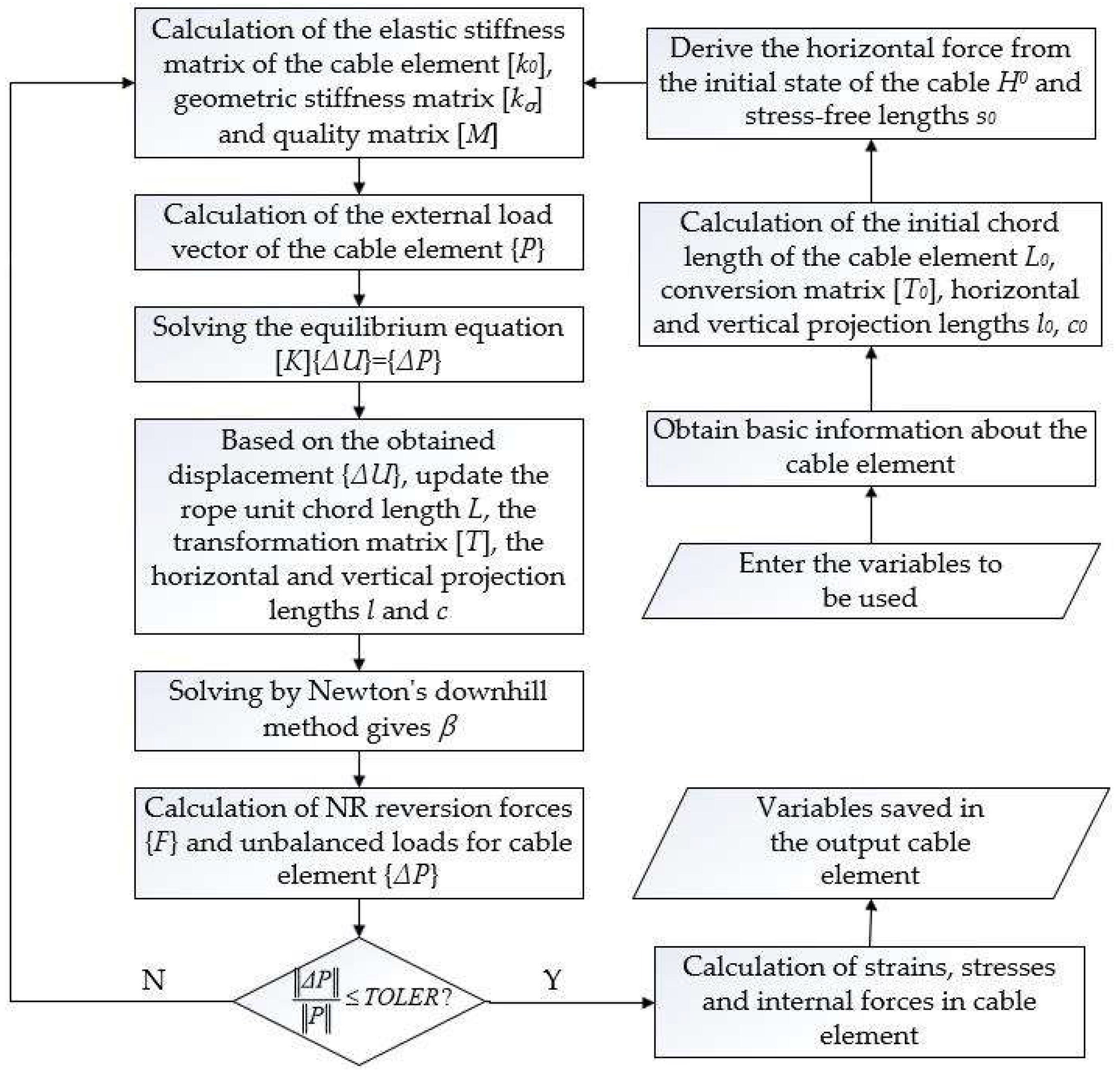
3. User Element Secondary Development Process
- (1)
- Enter the variables to be used in the cable element;
- (2)
- Obtain basic information about the cable element: modulus of elasticity E, area A, Poisson’s ratio μ, density den, initial strain ε, temperature Δt;
- (3)
- Call the function to calculate the initial chord length L0 of the cable element and the transformation matrix [T0], horizontal and projection lengths l0 and c0 based on the initial position of the cable element;
- (4)
- Solve for β0 with sufficient accuracy according to Equations (17) and (18) where the end force Ti or Tj is known and substituted into Equation (9) to derive the unstressed length s0 of the cable and the initial state horizontal force H0;
- (5)
- Calculation of the tangential stiffness matrix that is the elastic stiffness matrix [k0] and the geometric stiffness matrix [kσ], for the cable element in the structural coordinate system: when the first iteration is performed, the elastic stiffness matrix is calculated as in the linear analysis and the geometric stiffness matrix is 0; if it is not the first iteration, it is calculated according to Equation (3);
- (6)
- Calculation of the mass matrix [M];
- (7)
- Calculation of the external load vector P in the structural coordinate system;
- (8)
- Solve the equilibrium equation for the cable element according to Equation (6) for the unbalanced load, which is the external load vector {P}, at the first iteration;
- (9)
- Superimpose to the total displacement vector {U} of the cable element, based on the displacement increments {ΔU} obtained from the solution, and update the chord lengths of the cable element, the transformation matrix [T], and the horizontal and vertical projection lengths l and c.
- (10)
- Solve the constraint Equation (19) according to Newton’s downhill method to obtain β, substitute β into Equation (7) to obtain the cable end force, which is NR recovery force {F}, and the unbalanced load {ΔP};
- (11)
- The convergence of the force is judged by comparing the magnitude of the L2-van of the unbalanced force with the tolerance value TOLER; if it is less than or equal to TOLER, the program is considered to have converged. Otherwise, it returns to Step (5) to continue the operation; where the tolerance value TOLER is a minimal value, and the default is 0.001;
- (12)
- Calculation of strains and stresses in the rope element from the total displacement vector, followed by calculation of axial forces, etc.;
- (13)
- Outputs the variables saved by the cable element.
4. Verification and Numerical Examples
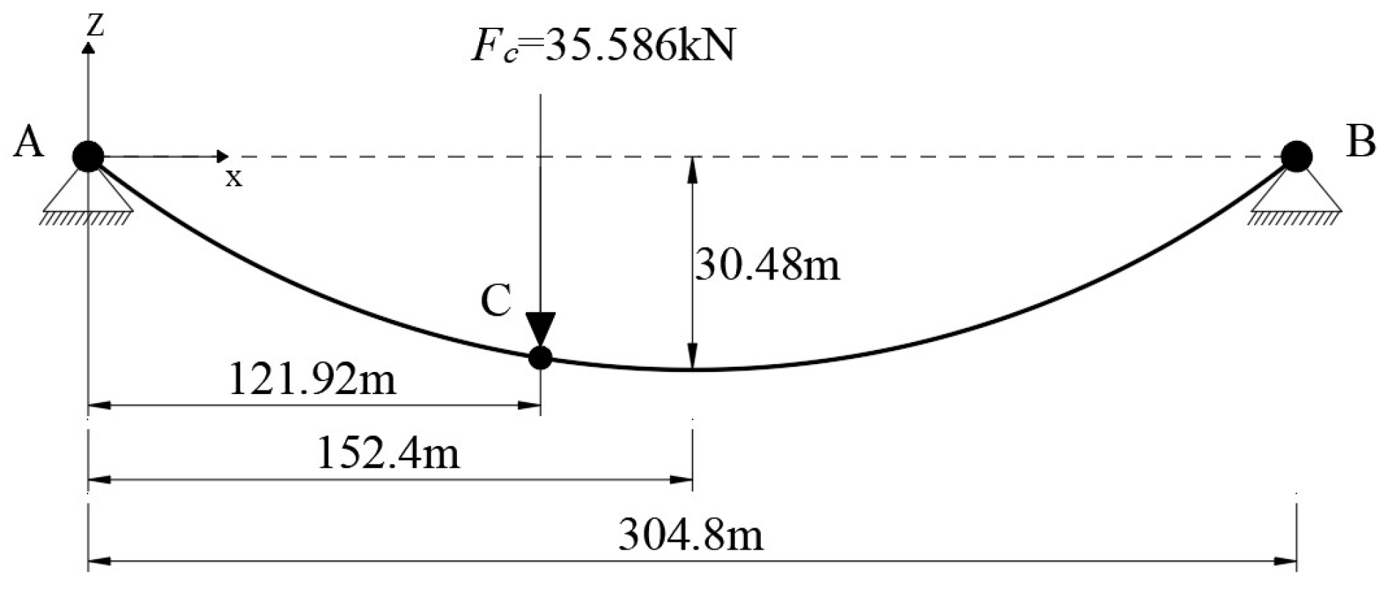
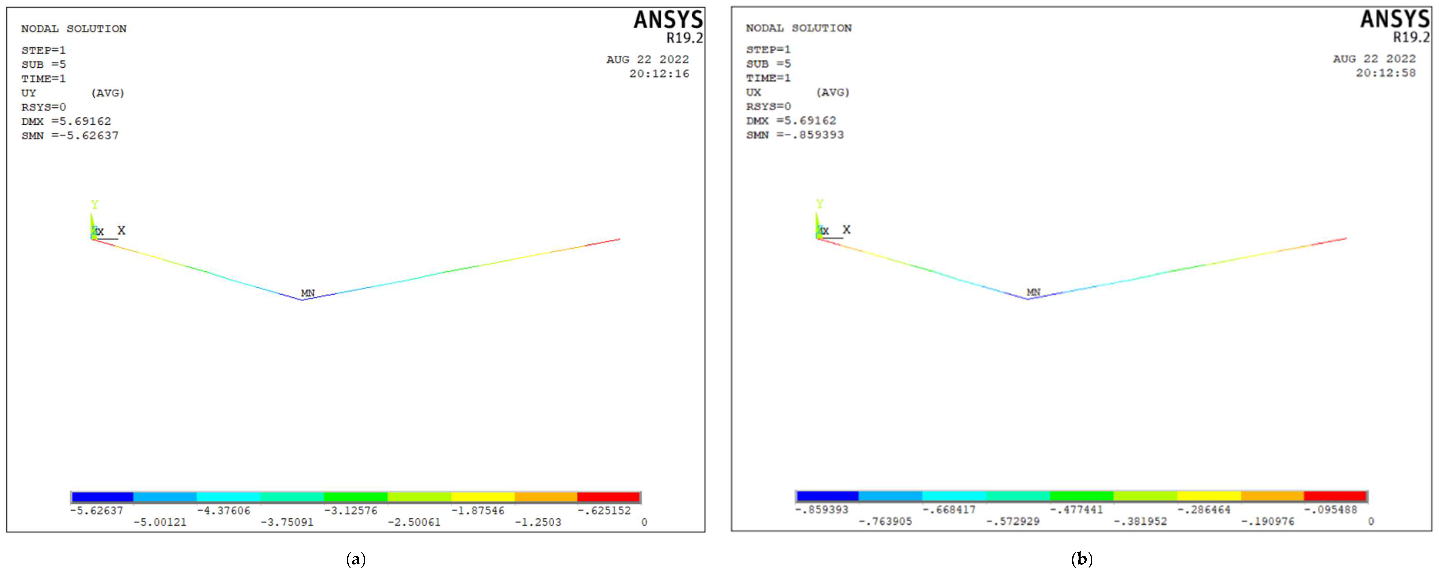
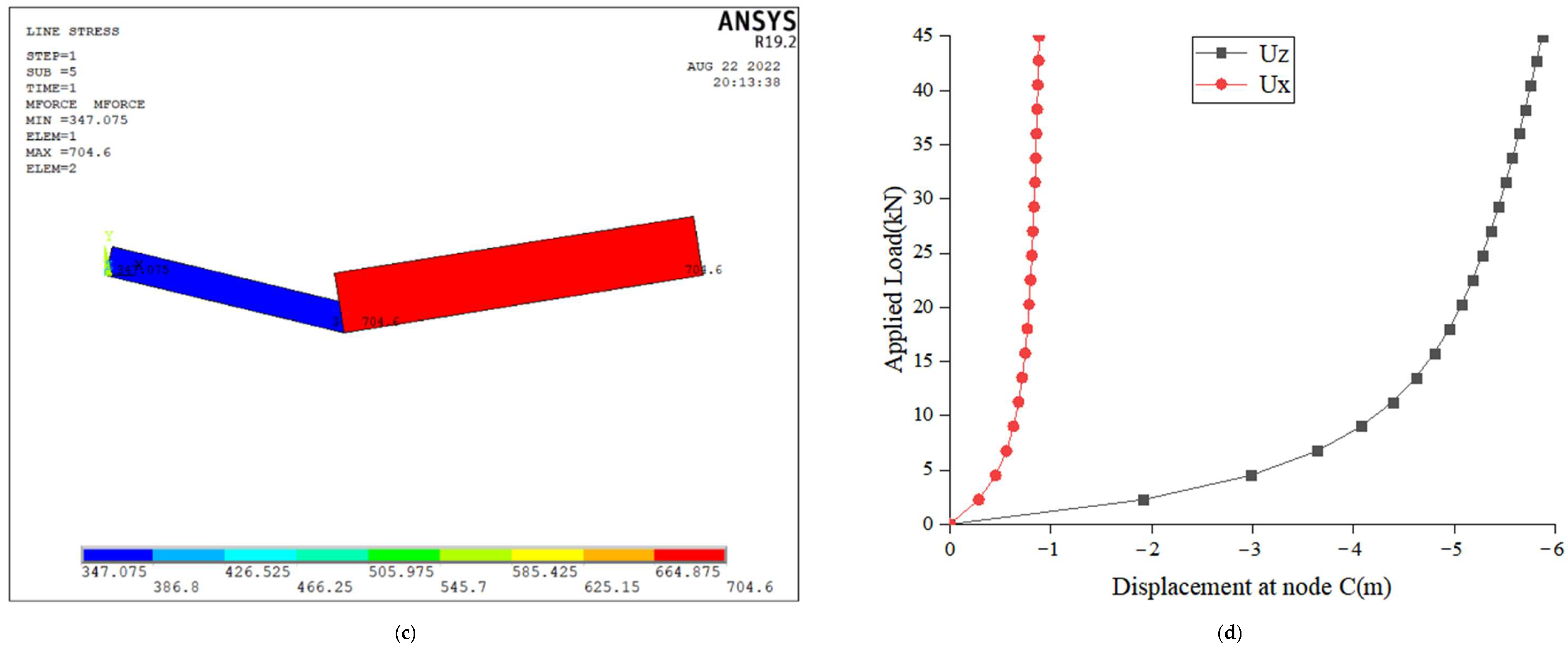
4.1. Single Cable Structures Subjected to Concentrated Loads
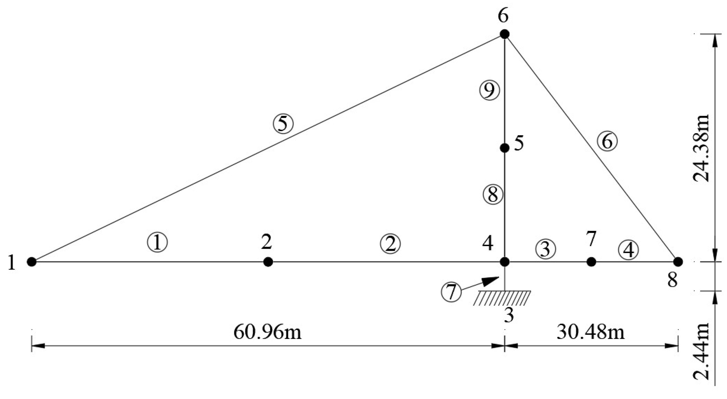
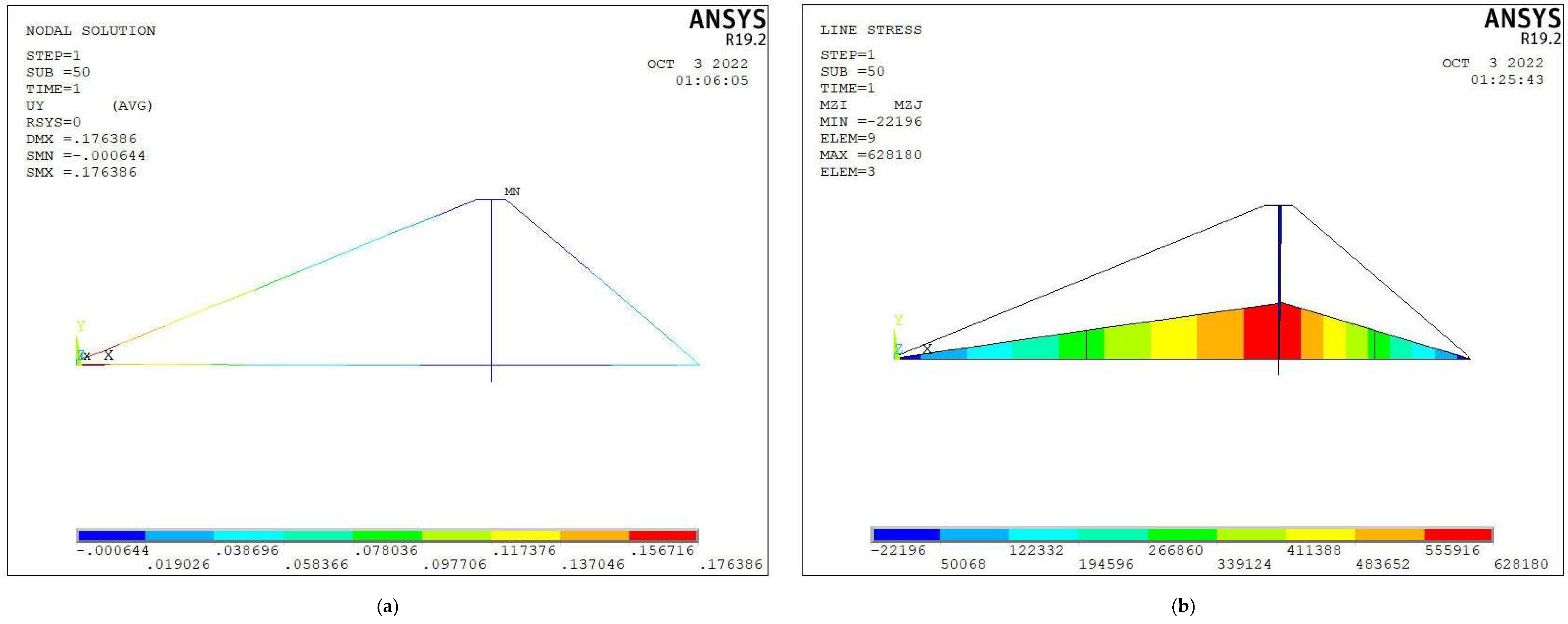
4.2. Verification and Analysis of Tensioned Cable Structures
- (1)
- The two cables are synchronized for initial tensioning at the end of the tower, with the initial tension of 27,154 kN for the left-hand cable, that is, element No. 5, and 33,037 kN for the right-hand cable, that is, element No. 6, anchored after tensioning is completed;
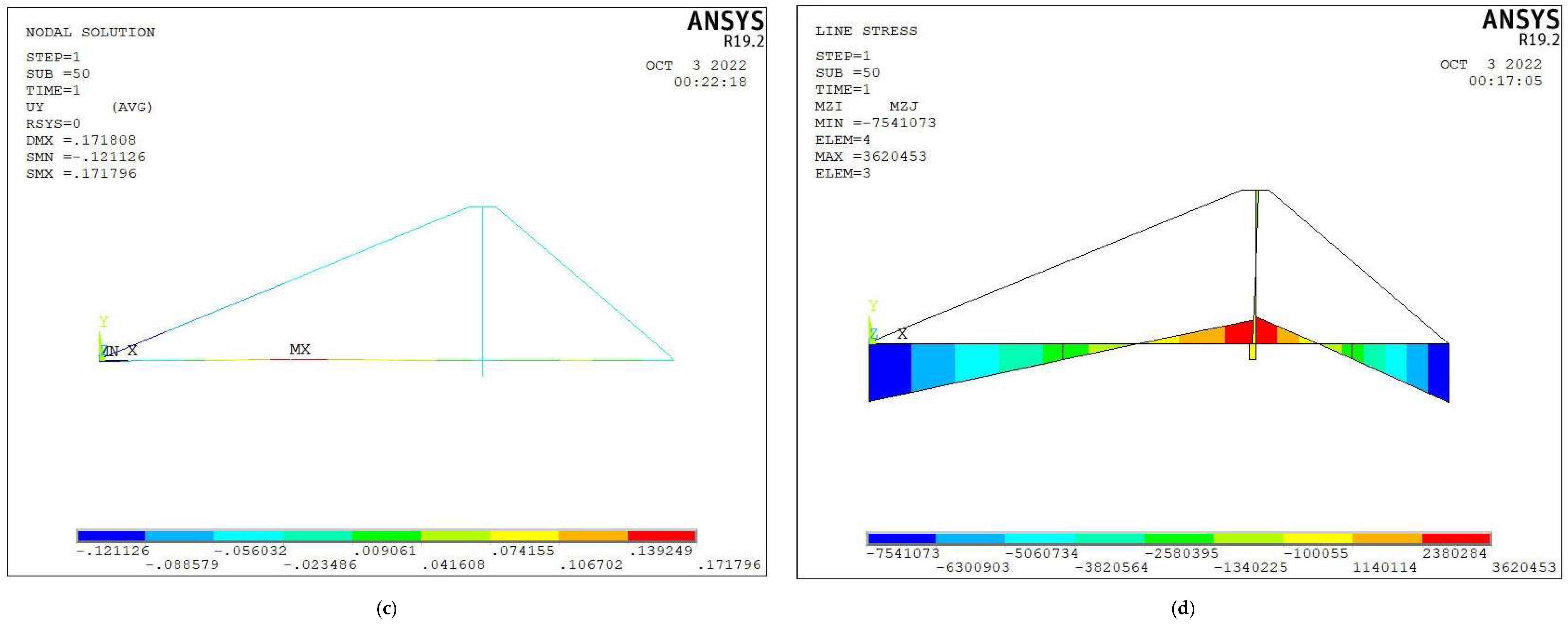
- (2)
- A concentrated force couple of 8 × 10⁶ kN·m is applied simultaneously at each of the two cantilevered ends of the main beam.
4.3. Engineering Example Validation and Analysis
5. Conclusions
- For the nonlinear analysis of cable structures, higher computational accuracy and efficiency are always the goals to be pursued, and when the pretension of the cable structure is high and involves network topology, the accurate initialization solution is essential for the convergence of the nonlinear structure, and this paper adopts the dichotomous method to iterate the initial configuration of the cable unit with pretension to accelerate the convergence and thus improve the computational efficiency.
- Through the comparison and verification between the example and the engineering model, it can be seen that, according to the characteristics of large span cable-stayed bridges or arch bridges with cable-stayed suspension construction, the initial geometric configuration of the cable is first solved iteratively by the dichotomous method under the known initial tension of the cable, and then the equilibrium equation of the cable element is solved iteratively according to the nonlinear geometric algorithm of the two-node catenary cable element, so the catenary cable element user101 developed in this paper can be directly applied to the ANSYS model for analysis and calculation;
- A new type of element, user101, developed by using the nonlinear finite element algorithm of the catenary cable element combined with the ANSYS secondary development platform (UPFs), has a certain improvement in nonlinear calculation accuracy and efficiency compared to the existing commercial program ANSYS developed truss element, in order to save calculation time without reducing accuracy in the finite element calculation.
- More advanced algorithms can be combined with commercial procedures in subsequent work to develop more novel elements and also provide a new way of thinking for researchers to improve the usefulness of nonlinear theory.
Author Contributions
Funding
Institutional Review Board Statement
Informed Consent Statement
Data Availability Statement
Conflicts of Interest
References
- Coda, H.B.; Silva, A.P.O.; Paccola, R.R. Alternative active nonlinear total Lagrangian truss finite element applied to the analysis of cable nets and long span suspension bridges. Lat. Am. J. Solids Struct. 2020, 3, 17. [Google Scholar] [CrossRef]
- Dang, N.S.; Rho, G.T.; Shim, C.S. A Master Digital Model for Suspension Bridges. Appl. Sci. 2020, 10, 7666. [Google Scholar] [CrossRef]
- Wei, J.D.; Guan, M.Y.; Cao, Q.; Wang, R.B. Spatial combined cable element for cable-supported bridges. Eng. Comput. 2018, 36, 204–225. [Google Scholar] [CrossRef]
- Bruno, B.; Fa, G.Z.; Aloisio, A.; Pasca, D.; He, L.Q.; Fenu, L.G.; Gentile, C. Dynamic characteristics of a curved steel–concrete composite cable-stayed bridge and effects of different design choices. Structures 2021, 34, 4669–4681. [Google Scholar]
- Jose Antonio, L.G.; Xu, D.; Ignacio, P.Z.; Jose, T. Direct simulation of the tensioning process of cable-stayed bridges. Comput. Struct. 2013, 121, 64–75. [Google Scholar]
- Chen, Z.H.; Wu, Y.J.; Yin, Y.; Shan, C. Formulation and application of multi-node sliding cable element for the analysis of Suspen-Dome structures. Finite Elem. Anal. Des. 2010, 46, 743–750. [Google Scholar] [CrossRef]
- Nie, G.B.; Zhi, X.D.; Fan, F.; Shen, S.Z. Study of the tension formation and static test of a suspendome for Dalian Gymnasium. China Civ. Eng. J. 2012, 45, 43475. [Google Scholar]
- Francisco, M.; Miguel, O.; Antonio, C. Palma del Ro Arch Bridge, Crdoba, Spain. Struct. Eng. Int. 2010, 20, 338–342. [Google Scholar]
- Tian, Z.C.; Peng, W.P.; Zhou, C. High-Temperature Closure Control Technology of Concrete Arch Bridge Using Cable-Stayed Buckle and Cantilever Construction Method. Appl. Mech. Mater. 2014, 3489, 1032–1037. [Google Scholar] [CrossRef]
- Ernst, H.J. Der E-Modul von Seilen unter berucksichtigung des durchhanges. Der Bauing. 1965, 40, 52–55. [Google Scholar]
- Knudson, W.C. Static and Dynamic Analysis of Cable Net Structures; University of California: Berkeley, CA, USA, 1971. [Google Scholar]
- Ali, H.M.; Abdel-Ghaffar, A.M. Modeling the nonlinear seismic behavior of cable-stayed bridges with passive control bearings. Comput. Struct. 1995, 54, 461–492. [Google Scholar] [CrossRef]
- Thai, S.; Kim, N.; Lee, J.H. Isogeometric cable elements based on B-spline curves. Meccanica 2017, 52, 1219–1237. [Google Scholar] [CrossRef]
- Yang, W.; Sheng, R.Z.; Chong, W. A finite element method with six-node isoparametric element for nonlinear analysis of cable structures. Appl. Mech. Mater. 2013, 2212, 1132–1135. [Google Scholar]
- Yuan, X.F.; Dong, S.L. Nonlinear analysis of two-node curve-cable elements. Eng. Mech. 1999, 4, 59–64. [Google Scholar]
- Yang, M.G.; Chen, Z.Q. A nonlinear finite element method for fine analysis of two-node curved trail elements. Eng. Mech. 2003, 1, 42–47. [Google Scholar]
- Gründig, L.; Bahndorf, J. The design of wide-span roof structures using micro-computers. Comput. Struct. 1988, 30, 495–501. [Google Scholar] [CrossRef]
- Haber, R.B.; Abel, J.F. Initial equilibrium solution methods for cable reinforced membranes part I—Formulations. Comput. Methods Appl. Mech. Eng. 1982, 30, 263–284. [Google Scholar] [CrossRef]
- Gwon, S.G.; Choi, D.H. Three-Dimensional Parabolic Cable Element for Static Analysis of Cable Structures. J. Struct. Eng. 2015, 142, 06015004. [Google Scholar] [CrossRef]
- Song, Y.H.; Kim, M.Y. Comparison Study of Elastic Catenary and Elastic Parabolic Cable Elements for Nonlinear Analysis of Cable-Supported Bridges. J. Korean Soc. Civ. Eng. 2011, 31, 361–367. [Google Scholar]
- Tibert, G. Numerical analyses of cable roof structures. In Trita-BKN. Bulletin; KTH: Stockholm, Sweden, 1999; p. 180. [Google Scholar]
- Mostafa, S.A.A.; Ahmad, S.; Vahab, E.; Alireza, N.R. Nonlinear analysis of cable structures under general loadings. Finite Elem. Anal. Des. 2013, 73, 11–19. [Google Scholar]
- Thai, H.T.; Kim, S.E. Nonlinear static and dynamic analysis of cable structures. Finite Elem. Anal. Des. 2010, 47, 237–246. [Google Scholar] [CrossRef]
- Wang, C.J.; Wang, R.P.; Dong, S.L.; Qian, R.J. A New Catenary Cable Element. Int. J. Space Struct. 2003, 18, 269–275. [Google Scholar]
- Yang, Y.B.; Tsay, J.Y. Geometric nonlinear analysis of cable structures with a two-node cable element by generalized displacement control method. Int. J. Struct. Stab. Dyn. 2007, 7, 571–588. [Google Scholar] [CrossRef]
- Yang, M.G.; Chen, Z.Q.; Hua, X.G. A new two-node catenary cable element for the geometrically non-linear analysis of cable-supported structures. Proc. Inst. Mech. Eng. Part C J. Mech. Eng. Sci. 2010, 224, 1173–1183. [Google Scholar] [CrossRef]
- Vu, T.V.; Lee, H.E.; Bui, Q.T. Nonlinear analysis of cable-supported structures with a spatial catenary cable element. Struct. Eng. Mech. 2012, 43, 583–605. [Google Scholar] [CrossRef] [Green Version]
- Kim, J.C.; Chang, S.P. Initial Equilibrium State Analysis of Cable Stayed Bridges Considering Axial Deformation. J. Korean Soc. Steel Constr. 2002, 14, 539–547. [Google Scholar]
- Kim, K.S.; Lee, H.S. Analysis of target configurations under dead loads for cable-supported bridges. Comput. Struct. 2001, 79, 2681–2692. [Google Scholar] [CrossRef]
- Karoumi, R. Some modeling aspects in the nonlinear finite element analysis of cable supported bridges. Comput. Struct. 1999, 71, 397–412. [Google Scholar] [CrossRef]
- Wei, K.; Zhang, L.X.; Li, N. Cable Elements for Numerical Analysis of Highline Cable System of Alongside Replenishment. Appl. Mech. Mater. 2013, 2308, 2847–2850. [Google Scholar] [CrossRef]
- Jayaraman, H.B.; Knudson, W.C. A curved element for the analysis of cable structures. Comput. Struct. 1981, 14, 325–333. [Google Scholar] [CrossRef]
- Greco, L.; Impollonia, N.; Cuomo, M. A procedure for the static analysis of cable structures following elastic catenary theory. Int. J. Solids Struct. 2014, 51, 1521–1533. [Google Scholar] [CrossRef] [Green Version]
- Zhou, Y.F.; Chen, S.R. Iterative Nonlinear Cable Shape and Force Finding Technique of Suspension Bridges Using Elastic Catenary Configuration. J. Eng. Mech. 2019, 145, 04019031. [Google Scholar] [CrossRef]
- Chen, C.S.; Yan, D.H.; Chen, Z.Q. Nonlinear analysis of two-node accurate catenary with rigid arms. Eng. Mech. 2007, 24, 29–34. [Google Scholar]
- Thongchai, P.; Chainarong, A.; Somchai, C. Analysis of Large-Sag Extensible Catenary with Free Horizontal Sliding at One End by Variational Approach. Int. J. Struct. Stab. Dyn. 2017, 17, 1750070. [Google Scholar]
- Crusells-Girona, M.; Filippou, F.C.; Taylor, R.L. A mixed formulation for nonlinear analysis of cable structures. Comput. Struct. 2017, 186, 50–61. [Google Scholar] [CrossRef]
- Andreu, A.; Gil, L.; Roca, P. A new deformable catenary element for the analysis of cable net structures. Comput. Struct. 2006, 84, 1882–1890. [Google Scholar] [CrossRef]
- Vanja, T.; Ivica, K. Static and dynamic analysis of a spatial catenary. Građevinar 2008, 60, 395–402. [Google Scholar]
- Chung, K.S.; Cho, J.Y.; Park, J.I.; Chang, S.P. Three-Dimensional Elastic Catenary Cable Element Considering Sliding Effect. J. Eng. Mech. 2011, 137, 276–283. [Google Scholar] [CrossRef]
- Naghavi-Riabi, A.R.; Shooshtari, A. A Numerical method to material and geometric nonlinear analysis of cable Structures. Mech. Based Des. Struct. Mach. 2015, 43, 407–423. [Google Scholar] [CrossRef]
- Rodrigo, S.C.; Armando, C.C.L.; Silva Renata, G.L.; Porcino, S.A.; Harley, F.V. Cable structures: An exact geometric analysis using catenary curve and considering the material nonlinearity and temperature effect. Eng. Struct. 2022, 253, 113738. [Google Scholar]
- Rezaiee-Pajand, M.; Mokhtari, M.; Masoodi, A.R. A novel cable element for nonlinear thermo-elastic analysis. Eng. Struct. 2018, 167, 431–444. [Google Scholar] [CrossRef]
- Croce, P. Equivalent Axial Stiffness of Horizontal Stays. Appl. Sci. 2020, 10, 6263. [Google Scholar] [CrossRef]
- Lee, J.H.; Park, T.W. Development of a three-dimensional catenary model using cable elements based on absolute nodal coordinate formulation. J. Mech. Sci. Technol. 2012, 26, 3933–3941. [Google Scholar] [CrossRef]
- Hüttner, M.; Máca, J.; Fajman, P. The efficiency of dynamic relaxation methods in static analysis of cable structures. Adv. Eng. Softw. 2015, 89, 28–35. [Google Scholar] [CrossRef]
- Bouaanani, N.; Marcuzzi, P. Finite Difference Thermoelastic Analysis of Suspended Cables Including Extensibility and Large Sag Effects. J. Therm. Stresses 2011, 34, 18–50. [Google Scholar] [CrossRef]
- Bouaanani, N.; Ighouba, M. A novel scheme for large deflection analysis of suspended cables made of linear or nonlinear elastic materials. Adv. Eng. Softw. 2011, 42, 1009–1019. [Google Scholar] [CrossRef]
- Deng, J.H.; Zhang, X.Z.; Xu, B.L.; Tian, Z.C. Geometric nonlinear plane beam element based on secondary development of ANSYS. Chin. J. Appl. Mech. 2021, 38, 1161–1168. [Google Scholar]
- Xu, B.L. Nonlinear Analysis of Structural Geometry Based on Secondary Development of ANSYS; Changsha University of Science and Technology: Changsha, China, 2018. [Google Scholar]
- Chen, Z.D. Large Deflection Theory of Truss Plate and Shell; Science Press: Beijing, China, 1996. [Google Scholar]
- Shi, F. A Detailed Explanation of Secondary Development and Application of ANSYS; China Water Conservancy Press: Beijing, China, 2012. [Google Scholar]
- Wang, P.H.; Tseng, T.C.; Yang, C.G. Initial shape of cable-stayed bridges. Comput. Struct. 1993, 46, 1095–1106. [Google Scholar] [CrossRef]
- Yan, D.H.; Tian, Z.C.; Li, X.W. Design of Computer Procedures for Bridge Structures; Press of Hunan University: Changsha, China, 1999. [Google Scholar]
- Peng, W.P. Research on Cable Force Optimization and Arch Ring Stress Control during Construction of Long-Span Cantilevered Concrete Arch Bridges; Changsha University of Science and Technology: Changsha, China, 2020. [Google Scholar]


| Researcher (s) | Present | Jayaraman & Knudson [31] | Tibert [21] | Rezai-Pajand [43] |
|---|---|---|---|---|
| Element type | Catenary elements | Truss | Elastic parabola | Catenary elements |
| Number of elements | 2 | 10 | 2 | 2 |
| Vertical displacement uz at point C | −5.62637 | −5.471 | −5.601 | −5.626 |
| Lateral displacement ux at point C | −0.859393 | −0.845 | −0.866 | −0.859 |
| Parameters | Lower Tower | Upper Tower | Main Beams | Tensioning Cable |
|---|---|---|---|---|
| A/m2 | 0.9290 | 0.2787 | 0.7432 | 0.1022 |
| I/m4 | 1.7262 | 0.1726 | 0.3884 | 0 |
| Element Number | Δai | Δbi | Δaj | Δbj |
|---|---|---|---|---|
| 11 | 0.5 | −0.53 | 2.104 | 0 |
| 12 | 2.104 | 0 | 0.5 | −0.053 |
| Initial Tensioning | Concentration Couple | |||||
|---|---|---|---|---|---|---|
| Δv1*/m | M2/kN·m | M3/kN·m | Δv1/m | M2/kN·m | M3/kN·m | |
| Development element user101 | 0.1764 | 612,145 | 628,180 | −0.1211 | 3,620,453 | 3,234,527 |
| ANSYS element | 0.1847 | 624,478 | 649,296 | −0.1248 | 3,630,024 | 3,432,105 |
| Chen [34] | 0.1763 | 612,039 | 628,102 | −0.121 | 3,610,762 | 3,234,485 |
| Wang [53] | 0.1783 | 613,973 | 629,048 | / | / | / |
| BDCMS * [54] | 0.1805 | 624,395 | 649,100 | −0.125 | 3,629,264 | 3,431,046 |
| Modulus of Elasticity E (MPa) | Poisson’s Ratio ν | Density ρ (kg/m3) | |
|---|---|---|---|
| Main arch ring | 3.95 × 10⁴ | 0.2 | 2602 |
| Abutment pier | 3.25 × 10⁴ | 0.2 | 2500 |
| Buckle tower | 2.14 × 10⁵ | 0.3 | 7850 |
| Buckle anchor cables | 2.03 × 10⁵ | 0.3 | 7850 |
| West Bank Buckle Number | Initial Tension (kN) | West Bank Anchor Cable Number | Initial Tension (kN) | East Bank Buckle Number | Initial Tension (kN) | East Bank Anchor Cable Number | Initial Tension (kN) | Area of Buckled Anchor Cable (m2) |
|---|---|---|---|---|---|---|---|---|
| X1 | 1402 | XMS1 | 920 | D1 | 1402 | DMS1 | 914 | 0.00264 |
| X2 | 1282 | XMS2 | 1103 | D2 | 1282 | DMS2 | 1088 | 0.00306 |
| X3 | 1303 | XMS3 | 1282 | D3 | 1303 | DMS3 | 1267 | 0.00306 |
| X4 | 1303 | XMS4 | 1289 | D4 | 1303 | DMS4 | 1239 | 0.00306 |
| X5 | 1353 | XMS5 | 1439 | D5 | 1353 | DMS5 | 1411 | 0.00306 |
| X6 | 1501 | XMS6 | 1668 | D6 | 1501 | DMS6 | 1649 | 0.00264 |
| X7 | 1402 | XMS7 | 1347 | D7 | 1402 | DMS7 | 1291 | 0.00264 |
| X8 | 1498 | XMS8 | 1490 | D8 | 1498 | DMS8 | 1441 | 0.00348 |
| X9 | 1449 | XMS9 | 1449 | D9 | 1449 | DMS9 | 1425 | 0.00348 |
| X10 | 1697 | XMS10 | 1676 | D10 | 1697 | DMS10 | 1614 | 0.00445 |
| X11 | 1749 | XMS11 | 1708 | D11 | 1749 | DMS11 | 1656 | 0.00445 |
| X12 | 1906 | XMS12 | 1854 | D12 | 1906 | DMS12 | 1770 | 0.00445 |
| X13 | 2155 | XMS13 | 2208 | D13 | 2155 | DMS13 | 2135 | 0.00445 |
| X14 | 2197 | XMS14 | 2301 | D14 | 2197 | DMS14 | 2218 | 0.00445 |
| X15 | 2260 | XMS15 | 2135 | D15 | 2260 | DMS15 | 2166 | 0.00445 |
| X16 | 2256 | XMS16 | 2362 | D16 | 2256 | DMS16 | 2272 | 0.00348 |
| X17 | 2101 | XMS17 | 2321 | D17 | 2101 | DMS17 | 2280 | 0.00348 |
| X18 | 2003 | XMS18 | 2011 | D18 | 2003 | DMS18 | 2093 | 0.00348 |
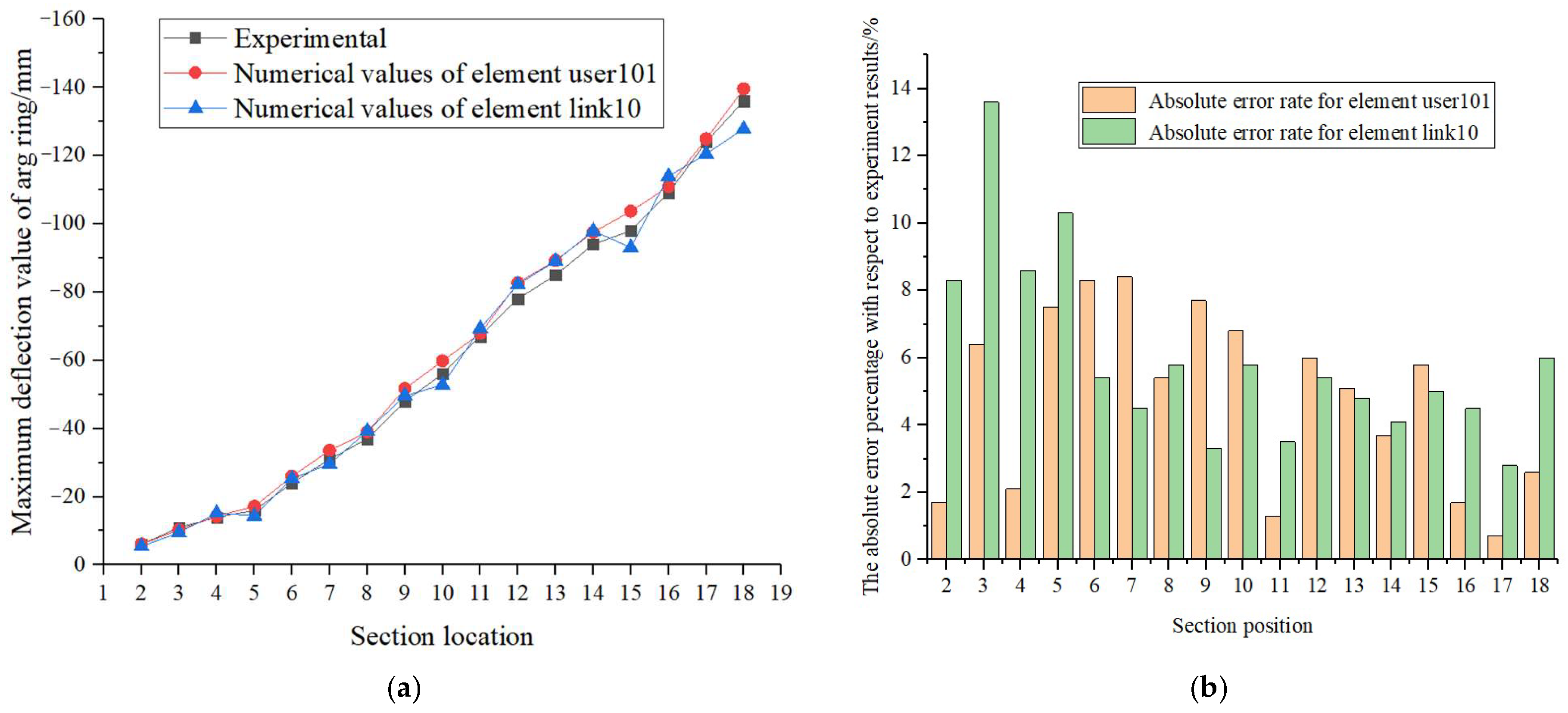
| Location of Measurement Points | Experiment/mm | Numerical Values (Development Element User101)/mm | Numerical Values (Ansys Element Link10)/mm |
|---|---|---|---|
| Section 2 | −6 | −6.1(1.7) * | −5.5(8.3) |
| Section 3 | −11 | −10.3(6.4) | −9.5(13.6) |
| Section 4 | −14 | −14.3(2.1) | −15.2(8.6) |
| Section 5 | −16 | −17.2(7.5) | −14.4(10.3) |
| Section 6 | −24 | −26.0(8.3) | −25.3(5.4) |
| Section 7 | −31 | −33.6(8.4) | −29.6(4.5) |
| Section 8 | −37 | −39.0(5.4) | −39.2(5.8) |
| Section 9 | −48 | −51.7(7.7) | −49.6(3.3) |
| Section 10 | −56 | −59.8(6.8) | −52.8(5.8) |
| Section 11 | −67 | −67.9(1.3) | −69.3(3.5) |
| Section 12 | −78 | −82.7(6.0) | −82.2(5.4) |
| Section 13 | −85 | −89.3(5.1) | −89.1(4.8) |
| Section 14 | −94 | −97.5(3.7) | −97.9(4.1) |
| Section 15 | −98 | −103.7(5.8) | −93.1(5.0) |
| Section 16 | −109 | −110.9(1.7) | −113.9(4.5) |
| Section 17 | −124 | −124.9(0.7) | −120.5(2.8) |
| Section 18 | −136 | −139.6(2.6) | −127.8(6.0) |
| Buckle Cable Number | Experiment /kN | Numerical Values (Development Element User101)/mm | Numerical Values (ANSYS Element Link10)/mm |
|---|---|---|---|
| X1 | 1501 | 1499(0.1) * | 1479(1.5) |
| X2 | 1434 | 1412(1.5) | 1398(2.5) |
| X3 | 1541 | 1499(2.7) | 1487(3.5) |
| X4 | 1550 | 1495(3.5) | 1506(2.8) |
| X5 | 1689 | 1621(4.0) | 1619(4.1) |
| X6 | 1843 | 1895(2.8) | 1786(3.1) |
| X7 | 1707 | 1657(2.9) | 1632(4.4) |
| X8 | 1834 | 1871(2.0) | 1772(3.4) |
| X9 | 1779 | 1757(1.2) | 1706(4.1) |
| X10 | 2129 | 2150(1.0) | 2018(5.2) |
| X11 | 2135 | 2048(4.1) | 2039(4.5) |
| X12 | 2338 | 2270(2.9) | 2235(4.4) |
| X13 | 2683 | 2576(4.0) | 2555(4.8) |
| X14 | 2772 | 2680(3.3) | 2613(5.7) |
| X15 | 2812 | 2659(5.4) | 2658(5.5) |
| X16 | 2765 | 2610(5.6) | 2646(4.3) |
| X17 | 2517 | 2426(3.6) | 2439(3.1) |
| X18 | 2180 | 2074(4.9) | 2092(4.0) |
Publisher’s Note: MDPI stays neutral with regard to jurisdictional claims in published maps and institutional affiliations. |
© 2022 by the authors. Licensee MDPI, Basel, Switzerland. This article is an open access article distributed under the terms and conditions of the Creative Commons Attribution (CC BY) license (https://creativecommons.org/licenses/by/4.0/).
Share and Cite
Xu, B.; Tian, Z.; Deng, J.; Zhang, Z. Geometric Nonlinear Analysis of the Catenary Cable Element Based on UPFs of ANSYS. Appl. Sci. 2022, 12, 9971. https://doi.org/10.3390/app12199971
Xu B, Tian Z, Deng J, Zhang Z. Geometric Nonlinear Analysis of the Catenary Cable Element Based on UPFs of ANSYS. Applied Sciences. 2022; 12(19):9971. https://doi.org/10.3390/app12199971
Chicago/Turabian StyleXu, Binlin, Zhongchu Tian, Jihua Deng, and Zujun Zhang. 2022. "Geometric Nonlinear Analysis of the Catenary Cable Element Based on UPFs of ANSYS" Applied Sciences 12, no. 19: 9971. https://doi.org/10.3390/app12199971
APA StyleXu, B., Tian, Z., Deng, J., & Zhang, Z. (2022). Geometric Nonlinear Analysis of the Catenary Cable Element Based on UPFs of ANSYS. Applied Sciences, 12(19), 9971. https://doi.org/10.3390/app12199971