Abstract
The introduction of modern methods for the mathematical processing of geological data is one of the promising areas of study and development in the field of geosciences. For example, today mathematical geology makes it possible to reliably identify astronomical cycles by measuring the scalar magnetic parameters of rocks (magnetic susceptibility). The main aim of this study is to develop a mathematical tool for identifying stable oscillation cycles (periods) in the dataset of the magnetic susceptibility of rocks in a geological section. The author’s method (algorithm) is based on the concept of discrete mathematical analysis—an innovative mathematical approach to the analysis of discrete geological and geophysical data. Its reliability is also demonstrated, by comparison with the results obtained by classical methods: Fourier analysis, Lomb periodogram, and REDFIT. The proposed algorithm was applied by the authors to analyze the material of field geological studies of the Zhelezny Rog section (Taman Peninsula). As a result, stable cycles were determined for the Pontian and Lower Maeotian sedimentary strata of the Black Sea Basin (Paratethys).
1. Introduction
In recent years, the active development of various geodata acquisition techniques caused the accumulation of large amounts of heterogeneous data. As a result, nowadays in geosciences, there is a need for new mathematical methods and approaches to analyze accumulated data. This is especially actual in geology for the analysis and interpretation of complex phenomena, such as paleoenvironmental changes, sedimentation rates, and fluctuations in insolation [1].
The Maeotian stratigraphic scale of the Black Sea region is based on the determination of mollusk fauna, along with dates of the boundaries of regional stages and their subdivisions derived from various geochronology methods. However, some uncertainties remain which cause disputes and impede the performance of full-scale interregional comparisons and paleogeographic reconstructions. The solution to this problem is improving the stratigraphic dissection of the studied sediments and developing methods for dating rocks. They include one of the new directions in geology: cyclostratigraphy (dating of strata by astronomical cyclicity, recorded in scalar magnetic parameters), which is often used in combination with mathematical approaches.
Cyclostratigraphy is a new scientific domain in stratigraphy and sedimentology that deals with identifying, describing, correlating, and interpreting cyclic variations in the stratigraphic sequence. In particular, cyclostratigraphy involves applying this knowledge to geochronology by increasing the accuracy and resolution of chronostratigraphic units. It uses the astronomical cycles of the currently known periodicity and an interpretation of the sedimentation conditions. According to the astronomical theory of paleoclimates, largely developed by Milankovitch, cyclical changes in the Earth’s orbit (orbital cycles) are the main causes of climate change [2]. These cycles translate into climatic, oceanographic, sedimentary, and biological changes recorded in sedimentary deposits over geological time. Numerous case studies have shown that detailed analysis of sedimentary rocks allows these cycles to be identified with a high degree of confidence. An unprecedented high temporal resolution is available once the relationship between the sedimentary record and orbital forcing is established. This relationship provides a basis for the timing of the processes occurring in the Earth system [3].
The main task of cyclostratigraphy is to analyze the structure of sedimentary deposits and identify stable signals reflecting the orbital influence. An essential aspect of time series analysis in cyclostratigraphy is transforming raw data into the time domain using calibration points. Once the time series is established, mathematical methods can be used to detect orbital periodicities.
Determination of astronomical cyclicity using geochronological methods, including paleomagnetic reconstruction and lithological analysis, is possible by defining the magnetic susceptibility of sediments. Magnetic susceptibility depends on the amount of solar radiation reaching the Earth’s surface and reflects climatic fluctuations. Spectral analysis of scalar magnetic parameters allows the detection of long-term period oscillations of the Earth’s axis, the angle of inclination of the Earth’s axis to the plane of the ecliptic, and eccentricity. This method gives a possibility to define absolute ages of sediments with accuracy in the order of 20,000 to 400,000 years.
In this paper, the application of mathematical methods to solve some critical problems of cyclostratigraphy and paleogeography of Eastern Paratethys Maeotian sediments is proposed. It should be noted that Eastern Paratethys has, for many years, been the research subject of one of the authors of the present paper. The study is aimed at the analysis of sedimentation processes of the Eastern Paratethys by the identification of stable oscillation cycles in the magnetic susceptibility data. To identify such cycles (periods), the authors developed a mathematical algorithm that is based on the concept of discrete mathematical analysis (DMA). DMA is an innovative mathematical approach to the analysis of discrete geological and geophysical data that was developed at the Geophysical Center of the Russian Academy of Sciences [4].
DMA is a series of algorithms united by a common formal basis: fuzzy comparisons of numbers, a measure of proximity in discrete spaces, and a discrete limit. DMA was developed to create discrete equivalents of the concepts of classical mathematical analysis: for example, limit, continuity, smoothness, connectivity, monotonicity, and extremum. DMA methods and algorithms have proven to be useful in numerous studies related to the processing and analysis of various geological [5], geophysical [6,7], geomagnetic [8,9,10,11,12], seismological [13], and other data [14].
2. Materials and Methods
The modern development stages of geology show a clear trend towards solving problems using more and more complex mathematical approaches. So simple statistics is being replaced by multi-dimensional methods. The concept of stochastic processes changed our understanding of geological history and led to the development of geostatistics. Nonlinear models are replacing linear ones. The introduction of fractal sizes has led to the notion of chaotic behavior. The above methods contribute to the development of cyclostratigraphic studies. Here we should note that cyclic sequences are predictable [1].
The most frequently used mathematical methods in geology can be roughly divided into three groups:
- Time series analysis, including spectral analysis (Fourier, spectrogram, and wavelet analysis), autocorrelation, cross-correlation, smoothing, filtering, and extremum search.
- Multivariate data analysis, including multivariate distributions and cluster analysis.
- Statistical methods, such as statistical distributions, correlation, regression, and chi-square tests.
- Neural networks (including deep learning neural networks).
2.1. Classical Spectral Methods
Of the groups of mathematical methods listed above, the group ‘time series analysis’, especially spectral analysis, is important for solving cyclostratigraphy problems. A brief description of the spectral methods most commonly used in cyclostratigraphy is provided below.
Any time series can be analyzed in terms of its description in the frequency domain. The classical way to detect frequency components in time series is Fourier spectral analysis. The importance of each frequency component in the time series is established using paired sine and cosine waves. Cyclostratigraphic data are discrete. For this reason, a discrete Fourier transform is applied. In a discrete Fourier transform, a time series is multiplied, point by point, by a cosine wave of a specific frequency. The results are summed and multiplied by a constant (2/N, where N is the number of points in the data series). This calculation gives the average amplitude of the cosine frequency component. The calculations continue assuming half the spectrum exists as a mirror image of the actual spectrum at ‘negative frequencies’. Since negative frequencies have no physical meaning for time series observations, the average amplitude must be doubled using a constant. The time series is then multiplied by a sine wave of the same frequency. The results are again summed and multiplied by a constant. For each frequency component investigated, the relative size of the average amplitude of the sine and cosine waves determines the average phase of the time series oscillations. Fourier transform can be considered as reorganizing time series data to a different location based on frequency.
To summarize, the Fourier transform is a mathematical operation that takes any waveform and breaks it down into separate sinusoidal components with different frequencies and amplitudes. The components are then presented as peaks in the frequency spectrum.
Spectral analysis of data series can be performed using the periodogram method. The periodogram is the square of the modulus of the amplitude of the Fourier spectrum. The Lomb periodogram is a frequency analysis technique for non-uniform data series. It is more suitable for cyclostratigraphic data than the Fourier transform. The Lomb periodogram is invariant concerning the time scale shift, and its statistical properties for non-uniform samples are equivalent to the Fourier transform properties for uniform samples. Frequency analysis by the Lomb method solves the problem of detecting oscillatory processes in data series. However, to study the evolution of the observed phenomena a time-frequency analysis is required. In this analysis, a subset of the sample is selected by a sliding observation window. When using an observation window, the data series is multiplied by a specific weight function [15].
Time series spectra are often characterized by a continuous decrease in spectral amplitude with increasing frequency (red noise). Additionally, time series are often unevenly distributed in time, making it difficult to estimate their red noise spectra. The REDFIT mathematical method [16] is an advanced version of the simple periodogram that solves this problem by directly fitting the first-order autoregressive process to unevenly distributed time series. In this way, the method avoids interpolation in the time domain and its inevitable shift. REDFIT is used to test if peaks in the spectrum of a time series are significant against a background of red noise from a first-order autoregressive process.
2.2. DMA-Algorithm for the Identification of Periods in Data Arrays
Within the framework of this study, the authors have developed a mathematical algorithm to identify periods (stable cycles) in data arrays. The algorithm is based on the DMA concept. DMA was briefly discussed above. The developed algorithm makes it possible to evaluate the consistency of any positive number as the period of the original function. The best answers, if they exist, are declared the identified periods. For simplicity of presentation, below we will call the algorithm developed here the DMA-algorithm. Let’s move on to a rigorous mathematical description of the DMA-algorithm.
Suppose that a function f is given on the segment [a, b], and we want to understand what periods it has. The period T, ideal for f, is defined as follows: T is the period for f if ∀t, t + T ∈ [a, b] is true f(t) = f(t + T). In reality, the function f may not have any ideal period T, but it may have approximate periods. A description of approximate periods and how to determine them is provided below.
It is clear that the applicant for the period T must lie in the interval (0, (b − a)/2). For such a T and t ∈ [a, a + T), we denote by {f, T, t} the finite sequence {f(t), f(t + T), f(t + 2T),…}. Firstly, it is necessary to understand to what extent the sequence {f, T, t} can be considered constant, i.e., to determine the exponent of its constancy C{f, T, t} ≥ 0. The equality C{f, T, t} = 0 must correspond to the constancy of the sequence {f, T, t }.
Here we present three different constructions of the exponent C{f, T, t}.
The first construction is the variance D of the sequence {f, T, t} relative to the usual or average median:
C{f, T, t} = D{f, T, t} or C{f, T, t} = Dm{f, T, t}.
The second and third constructions suppose the determination of the modulus of the difference sequence |∆{f, T, t}| for sequence {f, T, t}:
|∆{f, T, t}| = {|f(t + T) − f(t)|, |f(t + 2T) − f(t + T)|,…}.
The question of the constancy of {f, T, t} is reduced to the question of the triviality of |∆{f, T, t}|.
The second construction is the Kolmogorov mean Mp with a positive exponent p of the sequence |∆{f, T, t}|:
C{f, T, t} = Mp|∆{f, T, t}|.
As mentioned previously, using the Kolmogorov mean Mp, C indicates the proximity of the sequence |∆{f, T, t}| to zero.
Another solution is given by the third construction, using the distribution function F|∆{f, T, t}|:
where α(|∆{f, T, t}|) is α-quantile of the distribution F|∆{f, T, t}|.
C{f, T, t} = α(|∆{f, T, t}|),
The estimate C{f, T, t} characterizes T as a period on the sequence {t, t + T, t + 2T,…}.
The next stage is the development of a unified estimate T as a period independent of t. Such an estimate C(f, T) should be an indicator of the smallness of the set (C(f, T, t), t ∈ [a, a + T)). For this, we again use the Kolmogorov mean Mp:
C(f, T) = Mp(C(f, T, t), t ∈ [a, a + T)), p ≥ 0.
The final stage is the search for strong minima of the estimate C(f, T). Provided that they exist, we can obtain the necessary periods for the function f using the apparatus of minimality measures [4].
2.3. Time Series for the Demonstration of the Efficiency of the Algorithm
Figure 1 shows the time series that represents a series of oxygen isotopes of calcite in the shells of Pliocene and Pleistocene benthic foraminifera collected from 57 core samples worldwide [17]. This series contains the last 400,000 years of the record in 1000 year increments. This time series is comprehensively studied in numerous papers [17]. For this reason, we applied it below to demonstrate the efficiency of the described algorithms.
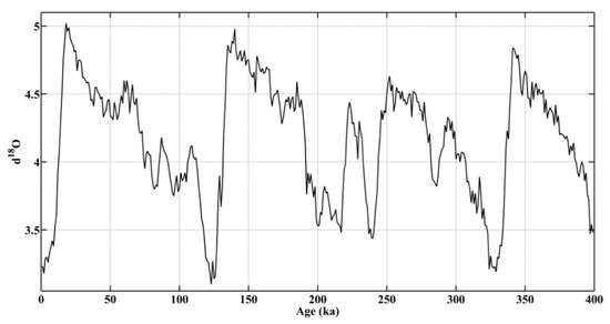
Figure 1.
Temporal fluctuations of the isotopic composition of precipitation [17].
2.4. Magnetic Susceptibility Data of Zhelezny Rog Cape
The objects of cyclostratigraphical study are deep-water sediments in the section of the Zhelezny Rog Cape of the Taman Peninsula, Black Sea Coast (N 45°11′06.1″, E 36°74′48.4″) [18,19]. Zhelezny Rog is a reference section of the Maeotian-Pontian and Pontian sediments of the European part of the Russian Federation.
Sediments of the Upper Maeotian, Upper and Lower Pontian up to 145 m were studied by the authors. The base of the Upper Maeotian is marked with a layer of clay breccia characterized by a homogeneous composition of clays and breccia clay matrix, and of the host sedimentary rocks, reflecting the underwater-colluvial origin of the considered sediments.
According to a micropaleontological study, the Upper Maeotian sediments are cyclically structured due to the influence of short-term inflows of seawater.
Beds with a monospecific assemblage of Actinocyclus octanarius diatoms are identified in the transitional layers between the Maeotian and Pontian [18,19]. Higher in the section, the number of diatoms is reduced.
The aleurite and non-calcareous clays occur higher and indicate the introduction of a river suspension and the stagnation of bottom waters. Subsequently, regression has led to the sandy clays deposition with a high kaolinite concentration.
The beginning of the Late Pontian is characterized by the breccia clays combined with horizons of shell-detrital limestones. The second half of the Late Pontian sediments consist of cyclic shallow-water clay.
In the present paper, we apply classical spectral methods and developed a DMA-algorithm to identify periods in magnetic susceptibility data of the Pontian (the total thickness of the sediments is 41.2 m; Figure 2a) and Lower Maeotian deposits (the total thickness of the deposits is 30 m; Figure 2b) of the Zhelezny Rog Cape. Measurements of the magnetic susceptibility of rocks were carried out using a field kappameter across the strike of the layers at regular intervals of 20 cm. Three measurements were taken at each point to ensure accuracy. For each point, the average susceptibility was calculated from the three measured values. The averaged magnetic susceptibility values are shown in Figure 2.
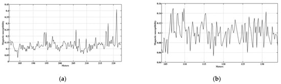
Figure 2.
Magnetic susceptibility of deposits of the Zhelezny Rog Cape section: (a) Lower-Upper Pontian; (b) Lower Maeotian.
3. Results
3.1. Demonstration of the Efficiency of the Algorithms
Figure 3a shows the Fourier and Lomb periodograms for the time series in Figure 1, which was previously normalized and centered. The Fourier periodogram is shown in blue, the Lomb periodogram is shown in red [20], and the spectrum obtained by the REDFIT method is shown in green in Figure 3b. Let us consider the observed Milankovitch cycles. Figure 3a shows that all six main peaks in the Fourier and Lomb periodograms are located at the frequencies (in decreasing order of spectral power): 0.0094, 0.0250, 0.0153, 0.0432, 0.0184, and 0.0339. This corresponds to the periods: 106,380 (eccentricity), 40,000 (tilt cycle), 65,360, 23,150 (precession), 54,350 and 29,500 years.
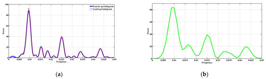
Figure 3.
(a) Fourier and Lomb periodograms; (b) REDFIT spectrum. Constructed for the time series in Figure 1.
The coincidence of the frequency maxima of the Fourier and Lomb periodograms (Figure 3a) can be explained by several factors. Firstly, the initial data have a uniform temporal distribution of observations. For data such as these, in the absence of white noise, there is an identical coincidence of the Fourier and Lomb periodograms [21]. Secondly, the differences in periodograms are caused by the presence of minor noise in the original data. The Lomb method [15] better distinguishes periods of 106,380 and 65,360 years from this noise.
The REDFIT spectrum (Figure 3b) shows five peaks at the frequencies (in descending order of spectral power): 0.0094, 0.0250, 0.0163, 0.0425, and 0.0325. Note that the two main peaks in the REDFIT spectrum are located at the same frequencies as the main peaks in the Fourier and Lomb periodograms. In this case, two REDFIT peaks are shifted in the frequency domain, and one peak combines two Fourier and Lomb peaks. The discrepancies may be because REDFIT considers the spectrum of red noise in the time series, which is not accounted for in the Fourier and Lomb transforms.
The results shown in Figure 3 demonstrate that spectral methods for studying time series are valuable tools in mathematical geology, particularly in cyclostratigraphy for detecting orbital periodicities.
On the example of time series presented in Figure 1, the efficiency of the developed DMA-algorithm is also demonstrated. Figure 4 shows the calculated constancy exponent of the series in blue and its smoothed version in red. As mentioned previously, the required periods of the time series are the points of the minimum of the constancy exponent C(f, T). Figure 4 shows that the strong periods are 115,000, 44,000 and 85,800 years. Weakly expressed periods are 58,600 and 67,600 years. Note that the identified periods are relatively close to the periods defined by spectral methods. Four out of five periods in Figure 4 closely match the periods in Figure 3. A possible explanation for the appearance of the 85,800 years period may be that it is a multiple of the 44,000 years period.
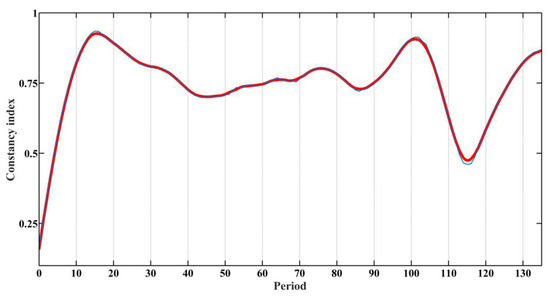
Figure 4.
Function constancy exponent (construction—variance) and determination of periods.
3.2. Identification of Periods in Magnetic Susceptibility Data
Figure 5 shows the results of applying spectral methods to the magnetic susceptibility data for the Pontian deposits (Figure 2a) of the Zhelezny Rog Cape. Of the three prominent peaks on the Lomb periodogram, two peaks fall within the 95% confidence interval (Figure 5a). These peaks are located at frequencies of 0.0425 and 0.2519, corresponding to periods of 23.53 m and 3.97 m, respectively. This result is confirmed by the Fourier periodogram (Figure 5a), where the main peaks are located at frequencies of 0.0437 and 0.2519 periods of 22.88 m and 3.97 m. In contrast to the example described above (Figure 3a), the Fourier and Lomb periodograms in Figure 5a differ slightly. These differences can be explained by white noise in the original data (Figure 2a).
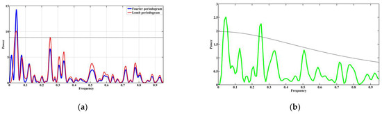
Figure 5.
The results of applying spectral methods to the magnetic susceptibility data from the Lower-Upper Pontian deposits of the Zhelezny Rog Cape section (Figure 2a): (a) Fourier and Lomb periodograms (the black bold solid line indicates the 95% confidence interval for the Lomb periodogram); (b) the spectrum constructed by the REDFIT algorithm (the black bold solid line indicates the 95% confidence interval).
Figure 5b shows the spectrum obtained using the REDFIT algorithm. Two peaks fall within the 95% confidence interval. They occur at frequencies of 0.0444 and 0.2525, which correspond to the periods of 22.52 m and 3.96 m. These periods coincide with the periods identified by the Fourier and Lomb periodograms.
Figure 6 shows the Fourier and Lomb periodograms and the REDFIT spectrum for the magnetic susceptibility data from the Lower Maeotian deposits (Figure 2b). Only one peak of the Lomb periodogram falls within the 95% confidence interval (Figure 6a). This peak is located at a frequency of 0.1408, which corresponds to a period of 7.1 m. This result is partially confirmed by the Fourier periodogram, where the main peak is at a frequency of 0.1516 (period 6.6 m). We are inclined to believe that the differences in the periodograms can be explained by noise in the data. The REDFIT spectrum is shown in Figure 6b. In this spectrum, just one peak is located in the 95% confidence interval. It occurs at a frequency of 0.1497, corresponding to a period of 6.68 m. The similarity in the periods obtained from the Fourier periodogram and the REDFIT spectrum may indicate more white noise than red noise in the initial data.
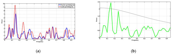
Figure 6.
The results of applying spectral methods to the magnetic susceptibility data of the Lower Maeotian deposits of the Zhelezny Rog Cape section (Figure 2b): (a) Fourier and Lomb periodograms (the black bold solid line indicates the 95% confidence interval for the Lomb periodogram); (b) the spectrum constructed by the REDFIT algorithm (the black bold dotted line indicates the 95% confidence interval).
To identify periods, the developed DMA-algorithm is applied. In Figure 7, the calculated constancy values for the magnetic susceptibility data of the Pontian and Lower Meotian deposits are shown in blue. As discussed previously, periods are considered to be the points of ‘global’ minima of the constancy exponent C(f, T). For this reason, the calculated constancy exponents were ‘strongly’ smoothed to obtain their global trends. The smoothed constancy exponents are shown as red lines in Figure 7. Figure 7a shows that the prominent period in the magnetic susceptibility data series of the Pontian deposits is 3.6 m. The minimum of the constancy exponent at 15.2 m can be considered a ‘weak’ period. The absence of the ~23 m period in Figure 7a is due to the algorithm considering values in half of the studied segment to be contenders for the period, which in this case is 41.2 m. For the Lower Meotian deposits, only one period of 7 m can be distinguished (Figure 7b). Strong periods in Figure 7 emerge as very close to the periods obtained using spectral methods of analyzing data series. In the case of a ‘softer’ smoothing of the constancy exponent (Figure 7), weaker periods can be obtained. In Figure 5 and Figure 6, these were not valid above the 95% confidence intervals or could not be obtained due to the low spatial resolution of the initial data.
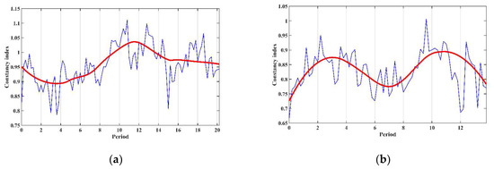
Figure 7.
The results of applying the developed DMA-algorithm to identify the periods in the magnetic susceptibility data for rocks of Zhelezny Rog Cape: (a) Lower-Upper Pontian deposits; (b) Lower Maeotian deposits. The calculated constancy exponent of the series is shown in blue (construction—dispersion, see above). The ‘strongly’ smoothed version is shown in red.
4. Conclusions
This paper presents new field data on the magnetic susceptibility of the Pontian and Lower Maeotian rocks of the Black Sea Basin (Paratethys), collected within the Zhelezny Rog section (Taman Peninsula, Russia). To identify stable periods in these data, the authors used both classical spectral algorithms and the DMA-algorithm developed in this paper.
In the studied interval, a 71-m-long sedimentary sequence, spectral analysis revealed statistically significant signals with some high peaks. These signals correspond to the precession and obliquity cycles. It should be noted that the 3.6 m peak corresponds to the precession periodicity (19–24 thousand years). The 7 m peak corresponds to the periods of changes in the angle of inclination of the Earth’s axis (41,000 years). The 15.2 m peak corresponds to the 100,000 year cycles; however, its validity is questionable due to the length of the interval (15 × 3 = 45 m). The 23 m peak is not valid, as the sampling interval is 41.2 m (cycle lengths are valid when they are three times the thickness of the interval: 23 × 3 = 69 m).
In the conclusion of the article, a few more words should be said about the mathematical apparatus, DMA [4]. It is the basis for the authors algorithm for the identification of periods in cyclostratigraphic data. The ideological mathematical basis of DMA-analysis allows the creation of algorithms for knowledge acquisition from geological and geophysical data. Based on fuzzy sets and fuzzy logic, DMA makes it possible to convey PC expert knowledge about the structure, morphology, monotony, etc. of studied data series. DMA enables a systematic approach to the analysis of complex data series of Earth sciences. Thereby DMA is a part of modern applied systems analysis [22].
Author Contributions
Conceptualization, A.I.R., B.A.D. and A.A.O.; data curation, A.A.O. and A.I.R.; methodology, A.I.R., B.A.D. and A.A.O.; software, B.A.D.; formal analysis, B.A.D. and B.V.D.; validation, A.I.R.; resources, A.I.R.; writing—original draft preparation, B.A.D., A.A.O. and B.V.D.; writing—review and editing, B.A.D., A.A.O., A.I.R. and B.V.D.; supervision, A.I.R.; project administration, A.I.R. and A.A.O.; funding Acquisition, A.I.R. All authors have read and agreed to the published version of the manuscript.
Funding
This research was funded by the Russian Science Foundation (project No. 19-77-10075).
Institutional Review Board Statement
Not applicable.
Informed Consent Statement
Not applicable.
Data Availability Statement
Not applicable.
Acknowledgments
The authors are grateful to employees of the Geophysical Center of the Russian Academy of Sciences, Sergey Agayan, Shamil Bogoutdinov and Dmitry Kudin for assistance with developing the algorithm and implementing the program code. This work employed data provided by the Shared Research Facility «Analytical Geomagnetic Data Center» of the Geophysical Center of RAS (http://ckp.gcras.ru/ (accessed on 15 December 2021)).
Conflicts of Interest
The authors declare no conflict of interest.
References
- Schwarzacher, W. Mathematical geology and the development of cyclostratigraphy. Geoinformatics 1993, 4, 353–356. [Google Scholar] [CrossRef][Green Version]
- Foucault, A. Sedimentary record of orbital cycles, methodology, results and perspectives. Bull. Soc. Geol. Fr. 1992, 163, 325–335. [Google Scholar]
- Strasser, A.; Hilgen, F.J.; Heckel, P.H. Cyclostratigraphy—Concepts, definitions and applications. Newsl. Stratigr. 2006, 42, 75–114. [Google Scholar] [CrossRef]
- Agayan, S.M.; Bogoutdinov, S.R.; Krasnoperov, R.I. Short introduction into DMA. Russ. J. Earth Sci. 2018, 18, ES2001. [Google Scholar] [CrossRef]
- Gvishiani, A.D.; Agayan, S.M.; Bogoutdinov, S.R.; Soloviev, A.A. Discrete mathematical analysis and applications in geology and geophysics. Vestn. KRAUNTs Nauk. Zemle 2010, 2, 109–125. [Google Scholar]
- Gvishiani, A.D.; Agayan, S.M.; Bogoutdinov, S.R. Discrete mathematical analysis and monitoring of volcanoes. Inzh. Ekol. 2008, 5, 26–31. [Google Scholar]
- Widiwijayanti, C.; Mikhailov, V.; Diament, M.; Deplus, C.; Louat, R.; Tikhotsky, S.; Gvishiani, A. Structure and evolution of the Molucca Sea area: Constraints based on interpretation of a combined sea-surface and satellite gravity dataset. Earth Planet. Sci. Lett. 2003, 215, 135–150. [Google Scholar] [CrossRef]
- Bogoutdinov, S.R.; Gvishiani, A.D.; Agayan, S.M.; Soloviev, A.A.; Kihn, E. Recognition of disturbances with specified morphology in time series. Part 1: Spikes on magnetograms of the worldwide INTERMAGNET network. Izv. Phys. Solid Earth 2010, 46, 1004–1016. [Google Scholar] [CrossRef]
- Gvishiani, A.; Soloviev, A.; Krasnoperov, R.; Lukianova, R. Automated Hardware and Software System for Monitoring the Earth’s Magnetic Environment. Data Sci. J. 2016, 15, 18. [Google Scholar] [CrossRef]
- Soloviev, A.A.; Bogoutdinov, S.R.; Agayan, S.M.; Gvishiani, A.D.; Kihn, E. Detection of hardware failures at INTERMAGNET observatories: Application of artificial intelligence techniques to geomagnetic records study. Russ. J. Earth Sci. 2009, 11, ES2006. [Google Scholar] [CrossRef]
- Gvishiani, A.D.; Lukianova, R.Y. Geoinformatics and observations of the Earth’s magnetic field: The Russian segment. Izv. Phys. Solid Earth 2015, 51, 157–175. [Google Scholar] [CrossRef]
- Gvishiani, A.D.; Mikhailov, V.O.; Agayan, S.M.; Bogoutdinov, S.R.; Graeva, E.M.; Diament, M.; Galdeano, A. Artificial intelligence algorithms for magnetic anomaly clustering. Izv. Phys. Solid Earth 2002, 38, 545–559. [Google Scholar]
- Gvishiani, A.D.; Dzeboev, B.A.; Agayan, S.M. FCAZm intelligent recognition system for locating areas prone to strong earth-quakes in the Andean and Caucasian mountain belts. Izv. Phys. Solid Earth 2016, 52, 461–491. [Google Scholar] [CrossRef]
- Gvishiani, A.D.; Agayan, S.M.; Bogoutdinov, S.R.; Zlotnicki, J.; Bonnin, J. Mathematical methods of geoinformatics. III. Fuzzy comparisons and recognition of anomalies in time series. Cybern. Syst. Anal. 2008, 44, 309–323. [Google Scholar] [CrossRef]
- Lomb, N.R. Least-squares frequency analysis of unequally spaced data. Astrophys. Space Sci. 1976, 39, 447–462. [Google Scholar] [CrossRef]
- Schulz, M.; Mudelsee, M. REDFIT: Estimating red-noise spectra directly from unevenly spaced paleoclimatic time series. Comput. Geosci. 2002, 28, 421–426. [Google Scholar] [CrossRef]
- Lisiecki, L.E.; Raymo, M.E. A Pliocene-Pleistocene stack of 57 globally distributed benthic δ 18O records. Paleoceanography 2005, 20, 1–17. [Google Scholar] [CrossRef]
- Rybkina, A.I.; Rostovtseva, Y.V. Astronomically-tuned cyclicity in Upper Maeotian deposits of the Eastern Paratethys (Zheleznyi Rog Section, Taman). Mosc. Univ. Geol. Bull. 2014, 69, 341–346. [Google Scholar] [CrossRef]
- Rostovtseva, Y.V.; Rybkina, A.I. The Messinian event in the Paratethys: Astronomical tuning of the Black Sea Pontian. Mar. Pet. Geol. 2017, 80, 321–332. [Google Scholar] [CrossRef]
- Hammer, Ø.; Harper, D.A.T. Paleontological Data Analysis; Blackwell Publishing: Hoboken, NJ, USA, 2005; Volume 351. [Google Scholar] [CrossRef]
- Carbonell, M.; Oliver, R.; Ballester, J.L. Power spectra of gapped time series: A comparison of several methods. Astron. Astrophys. 1992, 264, 350–360. [Google Scholar]
- Zgurovsky, M.Z.; Pankratova, N.D. System Analysis: Theory and Applications (Data and Knowledge in a Changing World); Springer: Berlin/Heidelberg, Germany, 2007; Volume 447. [Google Scholar] [CrossRef]


Publisher’s Note: MDPI stays neutral with regard to jurisdictional claims in published maps and institutional affiliations. |
© 2022 by the authors. Licensee MDPI, Basel, Switzerland. This article is an open access article distributed under the terms and conditions of the Creative Commons Attribution (CC BY) license (https://creativecommons.org/licenses/by/4.0/).