1. Introduction
With the continuous research on quantum communication, the structure and scale of quantum networks are changing dramatically. Quantum networks are no longer limited to regular network shapes but are developing toward large-scale, long-range, multi-user complex networks [
1,
2], which is determined by the future research and application prospects of quantum networks. The properties of quantum communication itself, such as Entanglement Swapping, also make it have better transmission performance than regular quantum networks under complex networks. Entanglement Swapping is the cornerstone of large-scale quantum networks. Relying on quantum repeaters in the network, Entanglement Swapping is able to overcome the exponential fading of quantum pairs over distance in the channel, allowing any two end nodes in the network to be connected. The connection between two nodes represents a pair of entangled qubits shared by these two nodes. Ideally, this pair of qubits would be in singlet state
, where
so that complete transmission of information
is ensured [
3]. However, in practical applications, the qubits in singlet state are affected by the environment, storage and channel noise, thus turning into a purely partially entangled state, making the transmission success probability
, resulting in unstable transmission of information. In complex quantum networks, the above problems can be amplified geometrically, causing serious impact on communication. Therefore, how to convert partially entangled state to singlet state (maximally entangled state) via LOCC (Local Operations and Classical Communications) while building complex quantum networks is our key concern [
4].
Similar to the traditional networks, quantum networks can be described in terms of graphs with similar properties. Specifically, a quantum network can be represented as
, where
is the set of nodes and
E is the set of edges contained in
, representing the communication nodes (including quantum relay nodes and end nodes) and the entangled connections between nodes in a quantum network, respectively. The entangled connections are in a singlet state in the ideal case and in a purely partially entangled state in the non-ideal case. For any node in the network, the number of nodes with which it has entangled connections is called the degree of the node, denoted as
k [
5]. Since we choose a small-world quantum network for research, the graphs under study also have a large clustering coefficient and a short average distance.
Percolation is a common phenomenon in complex networks: There is a certain value
for the connection probability
p between nodes in the network. When the connection probability is less than this value
, the nodes are slowly connected to form numerous small-scale connection clusters, and when the connection probability exceeds this value
, a Giant Connected Component (GCC), which basically runs through the whole network, will rapidly appear in the network. This certain value
is called the percolation threshold. For complex quantum networks, the percolation phenomenon occurs during the conversion from a partially entangled state to a maximally entangled state. When the conversion probability exceeds the percolation threshold of the network, we can quickly build a nearly fully connected quantum network, and this process is called Classical Entanglement Percolation (CEP) [
6]. Studies of percolation in classical complex networks have shown that the structure of the network affects the value of the percolation threshold to a large extent. Similarly, in complex quantum networks, as the edge reconnection occurs after entanglement swapping between the nodes and newly connected edges replace the original ones, both the structure of the network and the percolation threshold of the network are changed. Therefore, if we preprocess the network using entanglement swapping before the percolation occurs and lower the percolation threshold of the quantum network on purpose, we can establish the quantum communication network more efficiently. This is called Quantum Entanglement Percolation (QEP). After QEP, the change in the network structure is expressed as the change in the degree of nodes.
Preprocessing in small-world quantum networks can have problems: The nodes have different degrees and neighboring nodes have influence on each other because they share an edge, and the connected edges cannot be exchanged again once entanglement swapping is performed. Moreover, a reliable connection composed of maximally entangled state can be difficult for real application scenario, so the ConPT [
7] method is introduced and “sponge-crossing” probability is used to evaluate the percolation process instead of traditional size of clusters. In this paper, q-pswap is proposed to overcome these problems, and a central node is added when establishing the network in order to deal with the appearance of isolated nodes after entanglement swapping. Furthermore, the effects of ConPT methods are investigated so that the robustness of the network can be improved and the percolation threshold of the network can be reduced.
2. Percolation in Small-World Quantum Networks
A general quantum network composed of quantum nodes and connections are shown in
Figure 1. We consider a Watts–Strogatz (WS) small-world quantum network, as shown in
Figure 2, where any connected edge in the network is composed of a pure partially entangled state, where
.
can be converted to a maximally entangled state
with singlet conversion probability (SCP)
by LOCC.
is composed of two pure partially entangled states
, and its optimal SCP is
[
8]. Similar to the classical WS operation, the connected edges in the network are converted to maximally entangled state with a certain probability, and the connected edges (maximally entangled state) can be established between any two nodes in the connected cluster through entanglement swapping [
3].
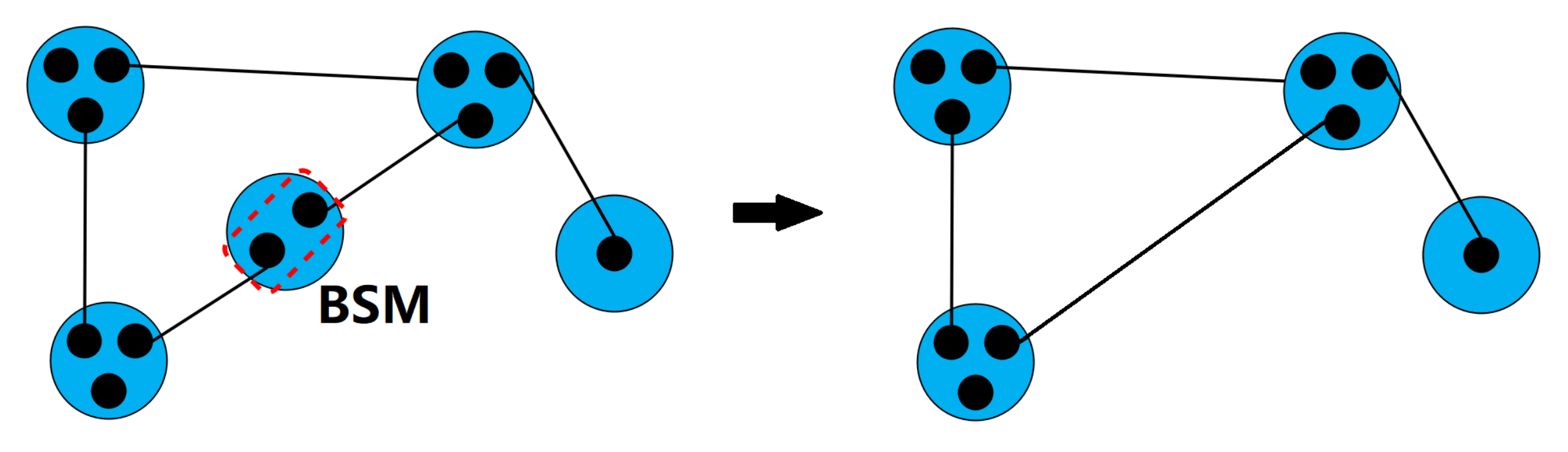
Before quantum percolation, quantum preprocessing will be performed [
8,
9], and the basic operation of quantum preprocessing is q-swap [
10], which performs an entanglement swapping on nodes with a degree of
q in the network (shown in
Figure 3). If an edge
has already undergone an entanglement swapping, then the newly generated edge is no longer
, so it cannot participate in the swapping operation again. Its SCP is identical to
. Different network structures change the percolation threshold of the network, therefore, quantum networks can change the network structure through quantum operations compared to classical ones [
10].
In regular networks, such as two-dimensional square lattice networks, triangular networks, cellular networks, etc., the nodes that perform preprocessing have the same degree and have no influence on each other when performing QEP. Unlike regular networks [
4], most of the nodes in a WS quantum network have different degrees, and since the edges after q-swap cannot be operated again, the q-swap of one node has an impact on neighboring nodes. WS small-world quantum networks have shorter average distances and larger clustering coefficients [
11].
3. Percolation Optimization
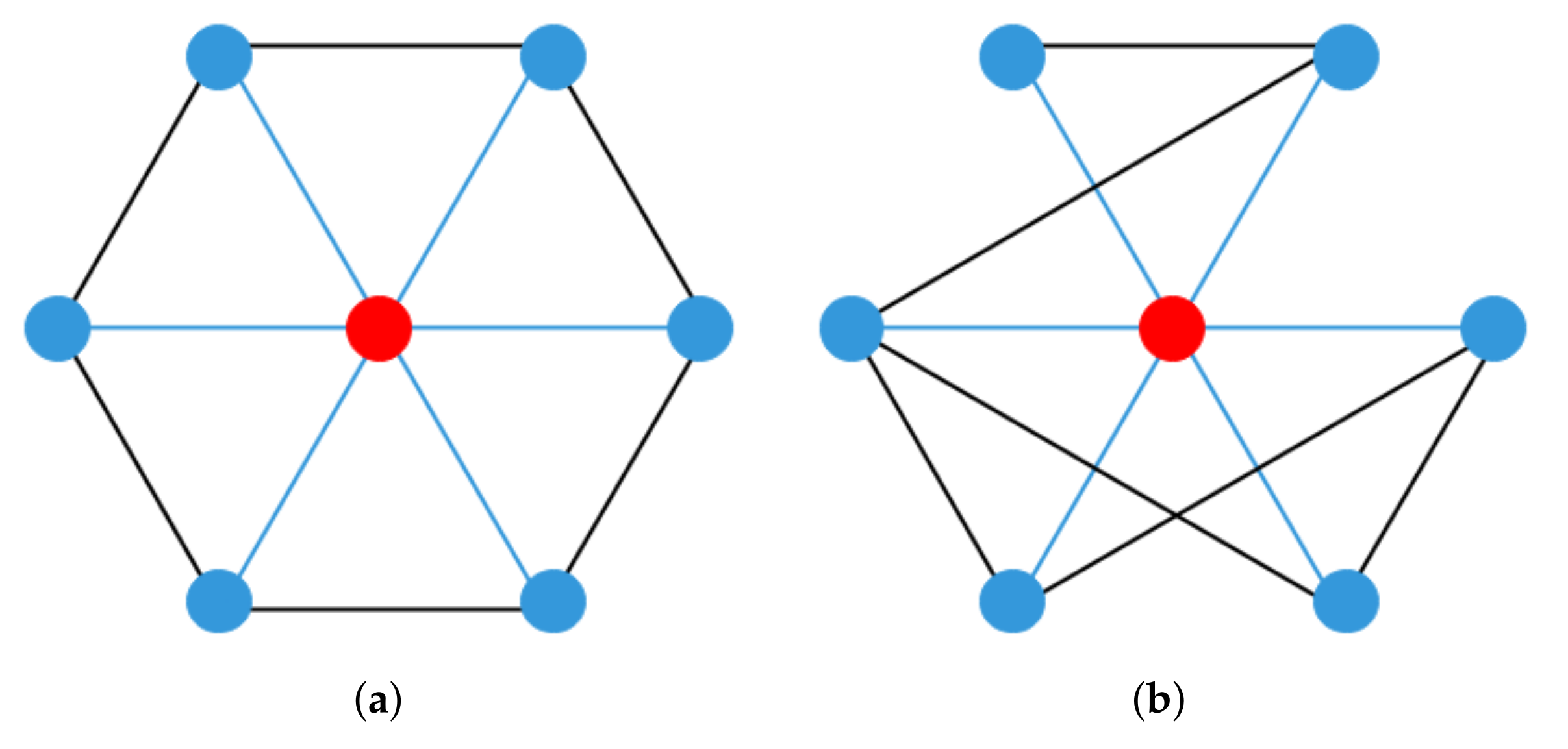
In order to ensure that any node in the network can be connected through entanglement swapping after percolation, we add a central node in the center of the network, which is connected to other nodes in the network. Taking a hexagonal network in a cellular network as an example, as shown in
Figure 4. In this case, fewer isolated nodes are made after entanglement percolation and most of the nodes in the network can communicate with others through entanglement swapping.
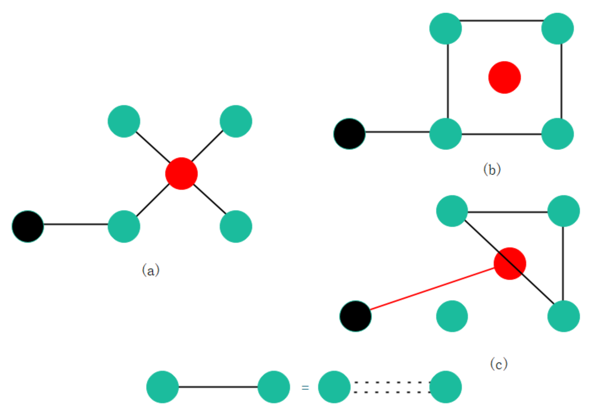
Partial q-swap (q-pswap) operation is shown in
Figure 5. For a node with a degree of four, entanglement swapping is only performed on part of the connected edges, and the rest of the connected edges can be swapped with the neighboring edges of other nodes, which can ensure that some important nodes do not become isolated nodes. At the same time, the impact of q-swap of one node on other nodes can be reduced.
The variation in GCC with edge conversion probability
p is an important property in the process of entanglement percolation of the network. For small-world quantum networks, there are several important statistical properties [
5]: clustering coefficient, degree distribution, and average shortest path. The clustering coefficient is a measure of the tendency of the nodes in a network to cluster together. The shorter the average shortest path, the fewer the number of entanglement swapping and resources are required by the nodes in the network to establish communication links.
We choose a WS quantum network with the number of nodes
, the reconnection probability of the network
, and the average network degree
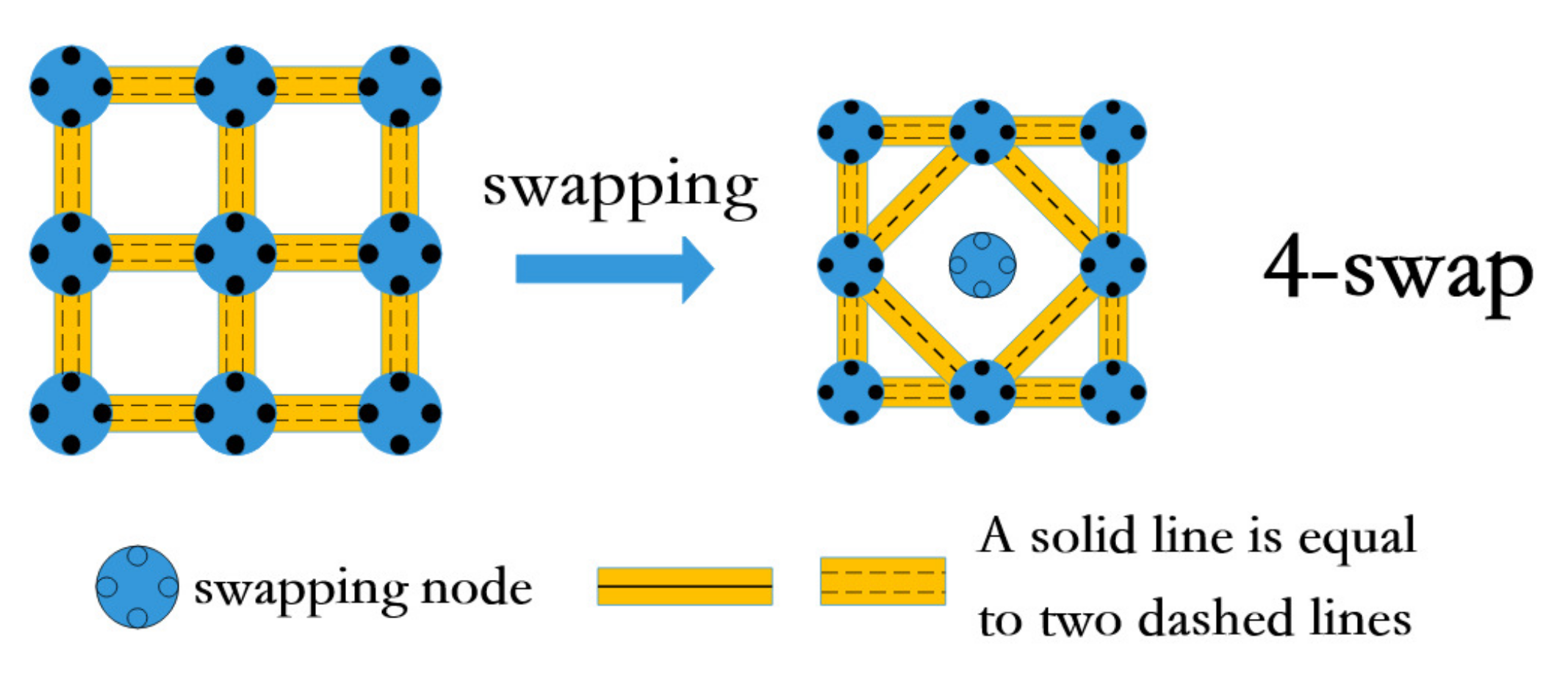
. After adding the central node, the average degree of the network becomes 6
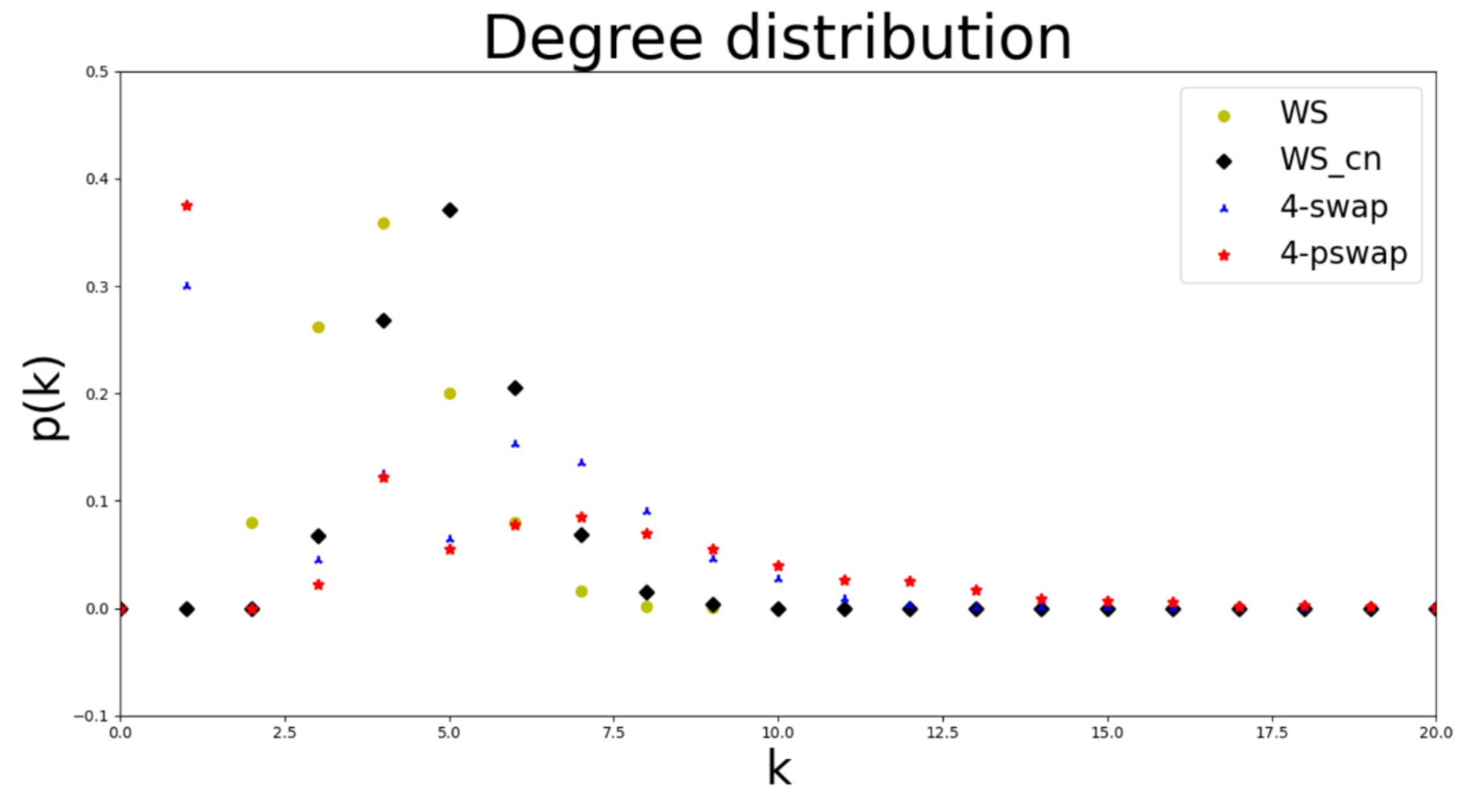
. In the process of disconnection–reconnection and quantum preprocessing, the connected edges of the central node are not involved in any operation. The central node is only used as an auxiliary node to ensure that there are not too many isolated nodes in the network and to reduce the average shortest path of the network and the resources required to establish connections. In the preprocessing process, we perform 4-swap as well as 4-pswap operations on nodes with a degree of 4. The degree distribution is shown in
Figure 6. Due to the existence of the central node, no isolated nodes will appear in the network. However, in the process of percolation, the connected edges of the central node will participate in the process, resulting in isolated nodes in the network. However, compared to the classical WS quantum networks, the addition of the central node can still reduce the appearance of isolated nodes. After 4-pswap, the degree distribution of the network is more uniform, and the probability of nodes with large degree values appears higher. In the process of percolation, nodes with larger degree values are more likely to percolate successfully.
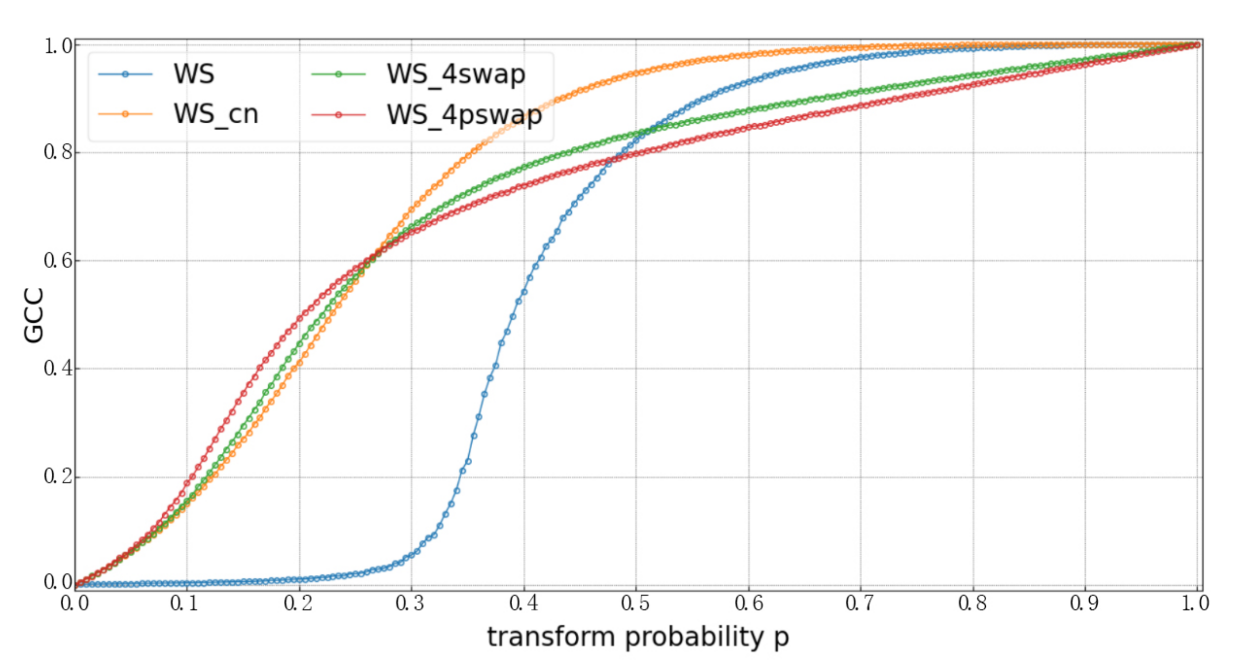
After the quantum preprocessing, the CEP operation is carried out. While changing the value of the edge conversion probability, the change in GCC in the network is observed (
, where
is the number of nodes contained in the giant connected cluster). As shown in
Figure 7, there is a significant decrease in the percolation threshold of the network due to the addition of the central node. So is the case after quantum preprocessing. The percolation threshold of the network after 4-pswap is lower compared to that after 4-swap. The clustering coefficient
implies the “cliquishness” of a small-world quantum network and is expressed as follows [
12]:
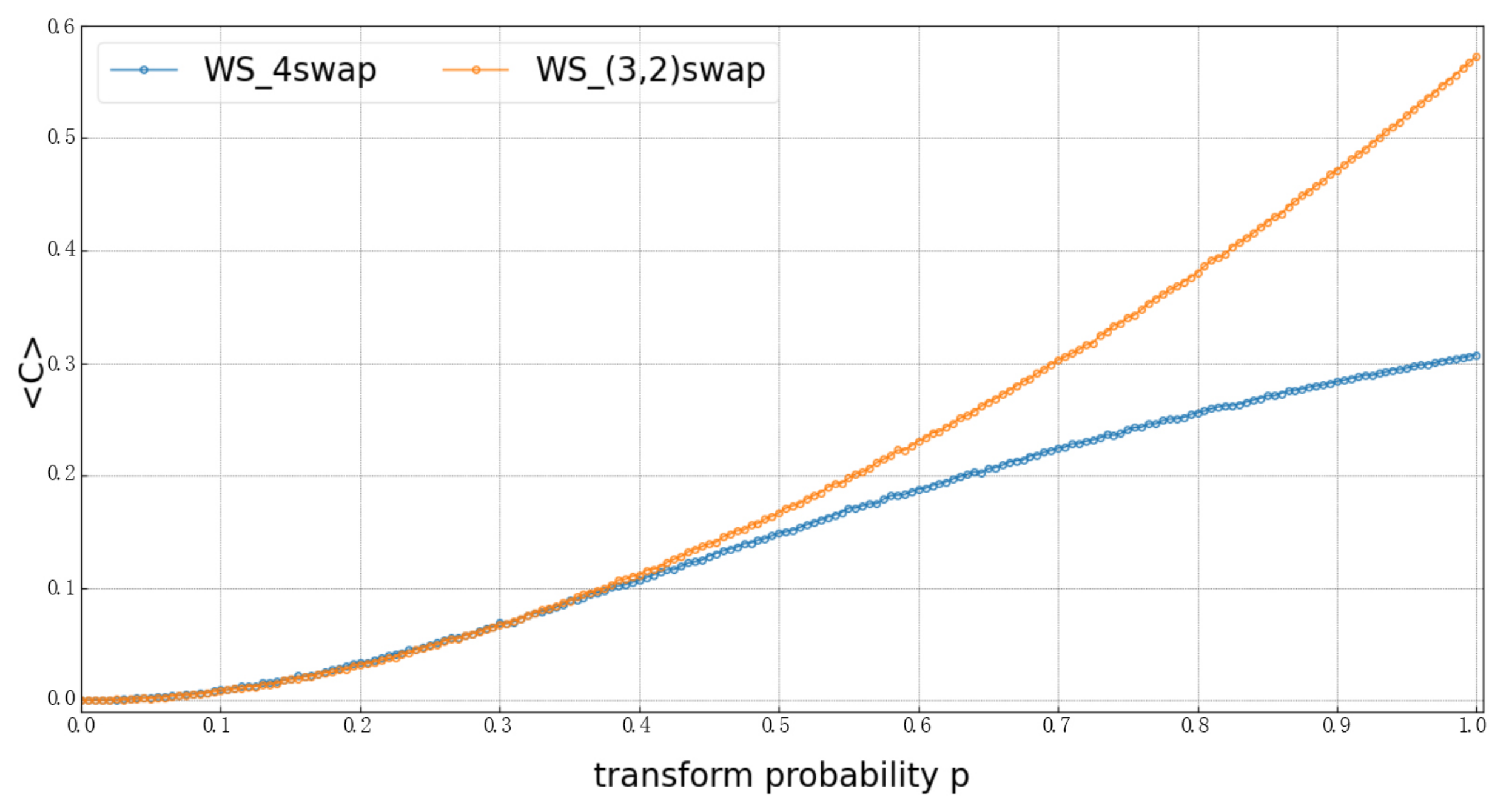
The relationship between the clustering coefficients of the networks obtained by different swap operations and the of edge conversion is shown in
Figure 8. It can be seen that the clustering coefficients
of the networks after (3, 2)-swap are larger compared to one after 4-swap, and the networks are more clustered. A (3, 2)-swap can be seen in
Figure 5c, in which swapping is performed on only three connected edges of the node with a degree of four, and the left one is swapped with peripheral nodes.
4. Concurrence Percolation in Small-World Quantum Networks
Whether using CEP or optimized QEP, a link composed of a singlet is required to accomplish communication between any two nodes in the network, and concurrence percolation [
13] can reduce the percolation threshold of the network while relaxing this condition. Concurrency is a metric of pure state entanglement, denoted as
(
c is defined as
for a pure state
, where
is the basis state) [
7]. Compared with traditional percolation analysis, concurrence percolation theory (ConPT) discards the measurement of cluster size and uses the “sponge-crossing” [
14] probability
, which is the probability that two distant nodes are interconnected by an open path.
can be calculated by combining the occupation probability of each path that connects two distant nodes using connectivity rules [
13]. The concurrency of “sponge-crossing” is denoted as
. According to the thermodynamic limit, both
and
should jump from 0 to 1 once approaching the percolation threshold
and
respectively [
13]. In the analysis of the network, the original network can be transformed by the following three rules to obtain the
and
of the network between two nodes.
Serial rule: for any 3 nodes A, B, J in the quantum network, A and J are connected by a link of concurrency
, while B and J are connected by a link of concurrency
. By performing a projection measurement on J (XZ is chosen as the measurement base), the final average concurrency obtained by the measurement is
Parallel rule: Nodes A and B are connected by two parallel links, which consist of product state, specified as:
when
, according to Nielsen’s theorem, the maximally entangled state can be obtained by conversion. The average concurrency obtained at this point
is optimal, where
is the probability that concurrency
obtained after measurement is in pure state.
Star-mesh (SM) transform: The star graph of size
n is transformed into a complete graph of size
, and then one node in the complete graph of
is selected as the root node to obtain a star graph of
. After several iterations, any two nodes in the connected cluster of the network share a connection. The series-parallel rule can be represented by
Table 1 [
13].
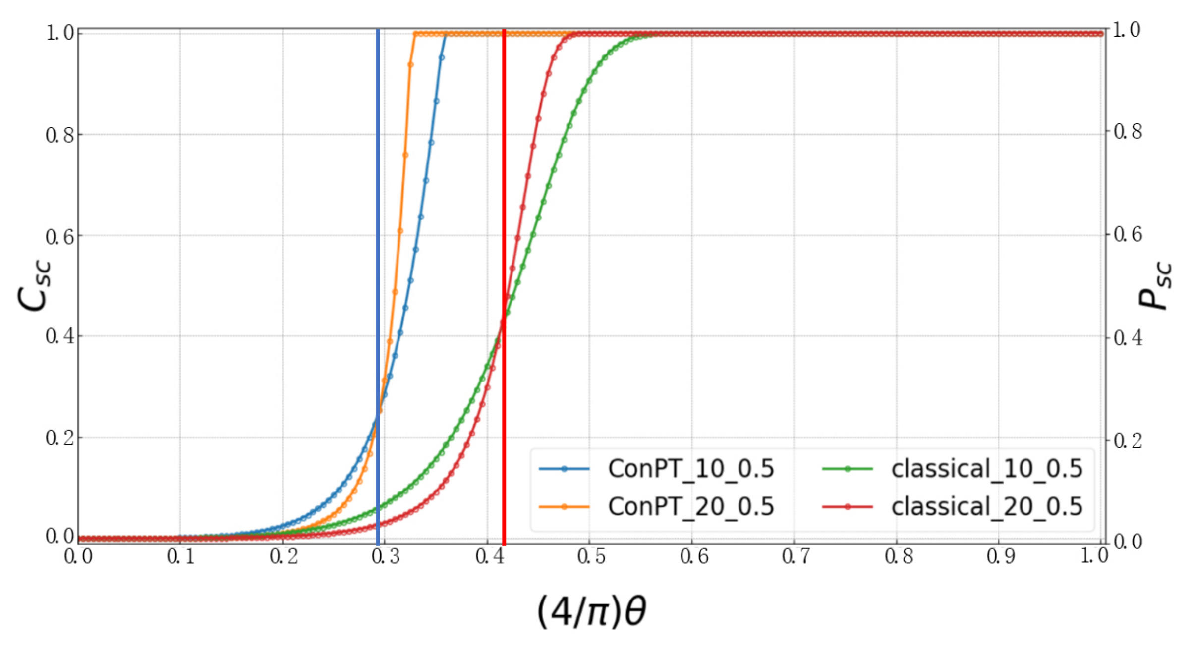
The above three methods are applied to the WS quantum network to analyze the percolation threshold of the network. The number of nodes in the WS quantum network are selected as
and
, the probability of reconnecting the network with disconnected edges
, the average degree of the network
, both ConPT and classical methods are simulated. As shown in
Figure 9, the percolation threshold obtained by the ConPT method is smaller:
and
.
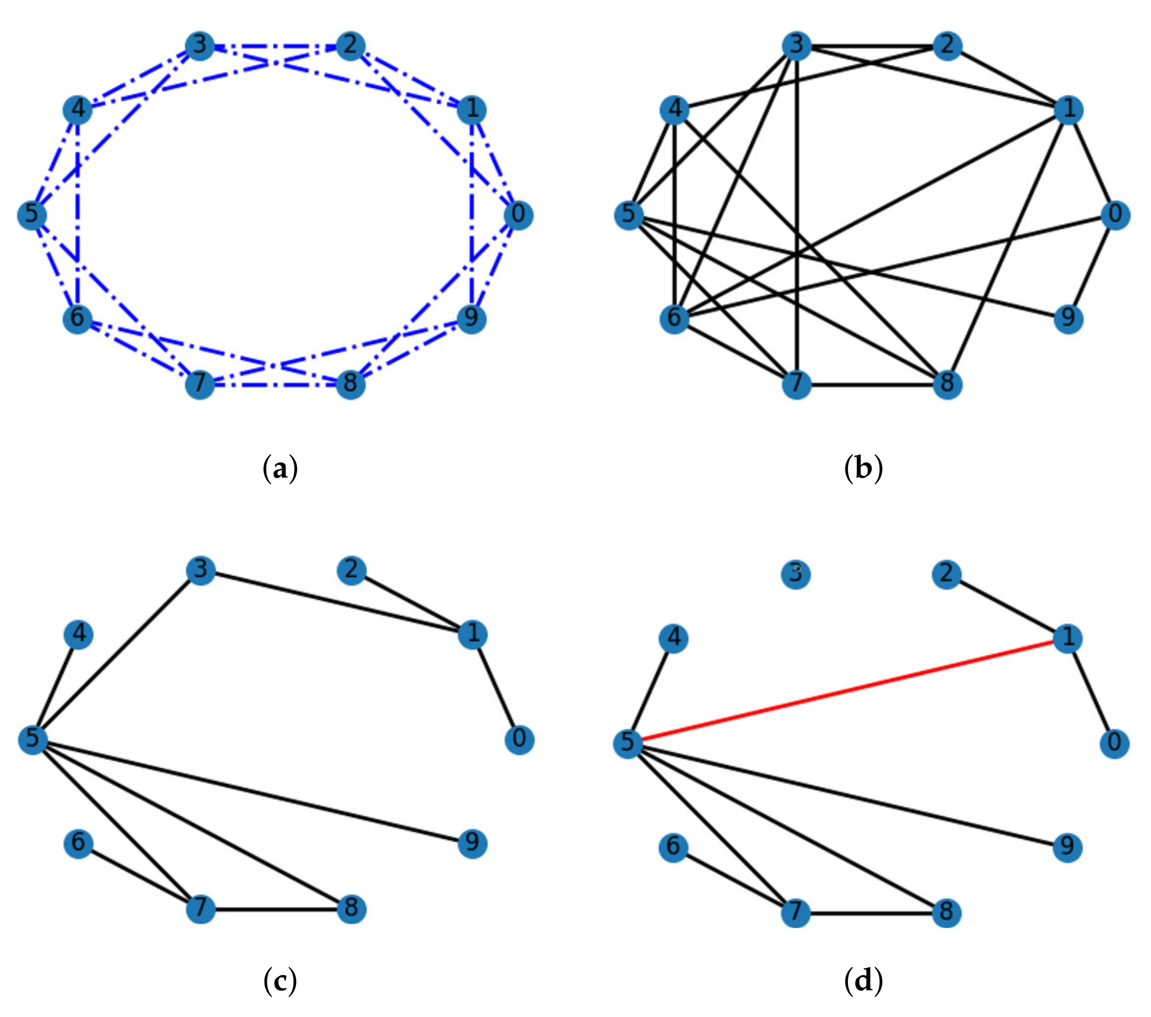
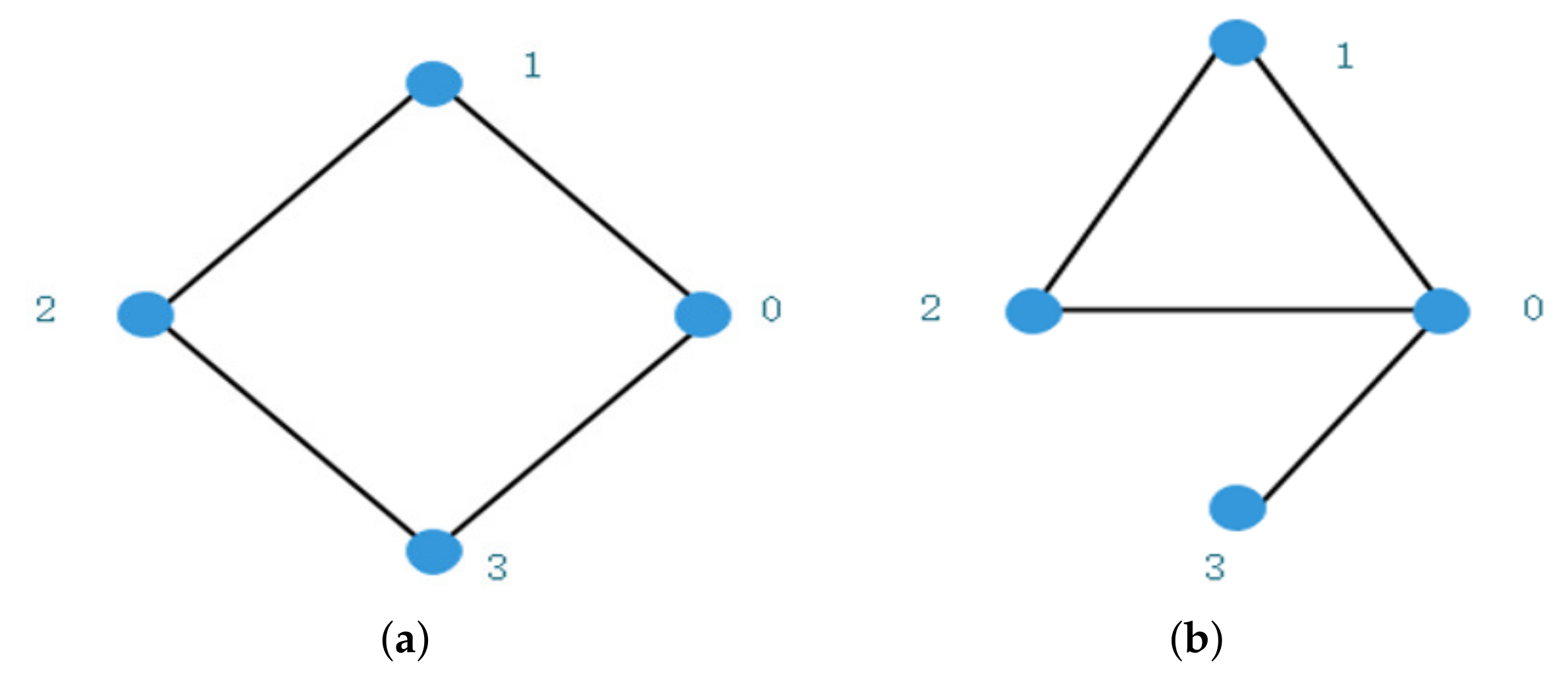
Unlike the structure of regular networks (e.g., cellular networks, Bethe lattice networks, etc.), WS quantum networks can have different topologies when different
are selected. Even if the same
is selected, the topologies obtained may be different as well. As shown in
Figure 10, the number of nodes, reconnection probability, and average degree are the same for both WS quantum networks. It is assumed that all connected edges
in these two networks have
and percolation from any node in the network will have little effect on the final obtained. Take the ConPT method as an example: We start from ConPT
in sequence with series-parallel rule and SM rule.
a obtained
, while
b obtained
. For the same parameters, different network topologies also obtain different
, which affects the percolation threshold.
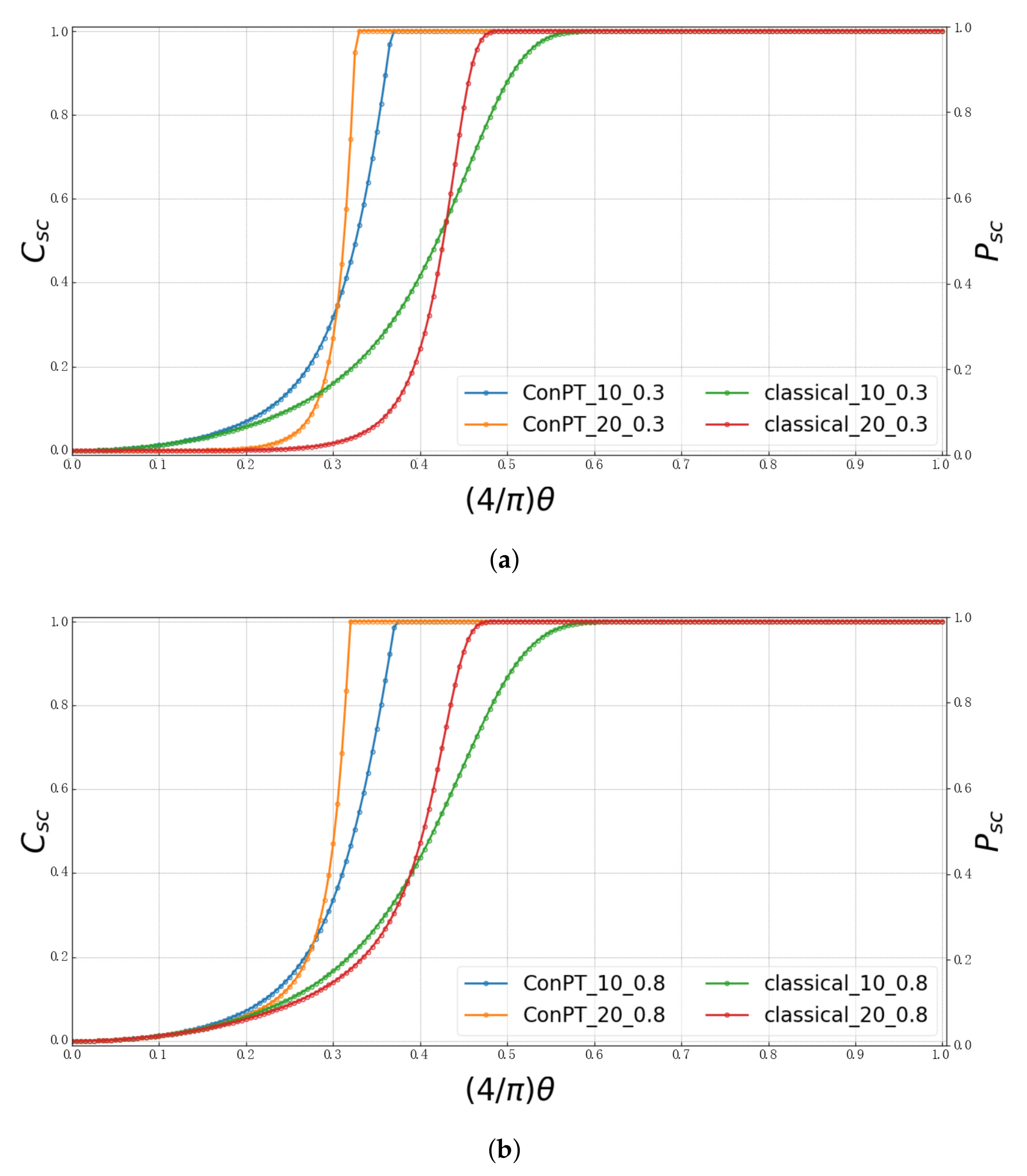
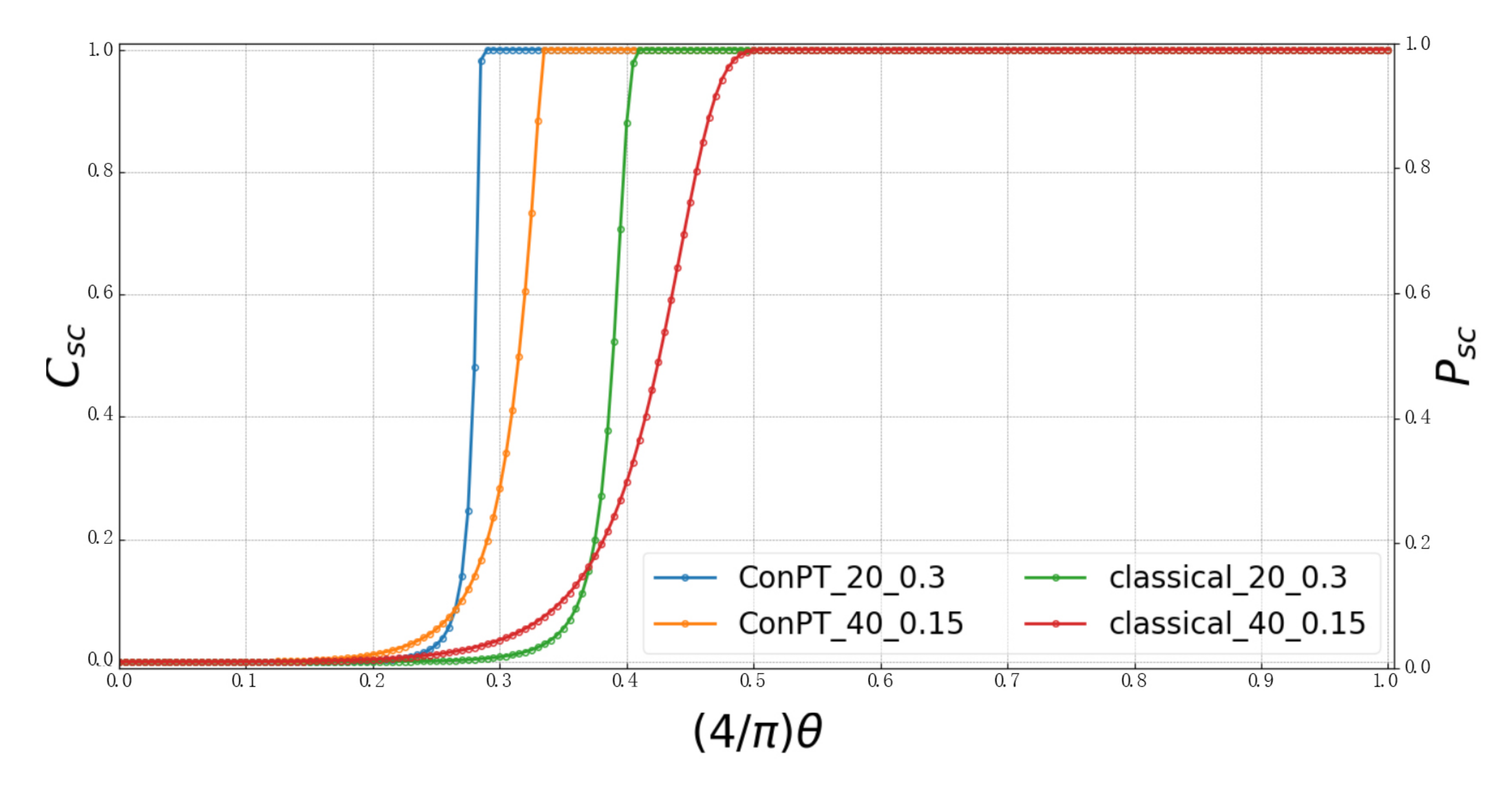
In order to analyze the effect of disconnection–reconnection probability
on the percolation threshold in WS quantum networks,
are selected. As shown in
Figure 11, when
,
,
and when
,
,
. With the increase in
, the percolation threshold of the network decreases gradually whether the network is percolated using the ConPT or classical method.
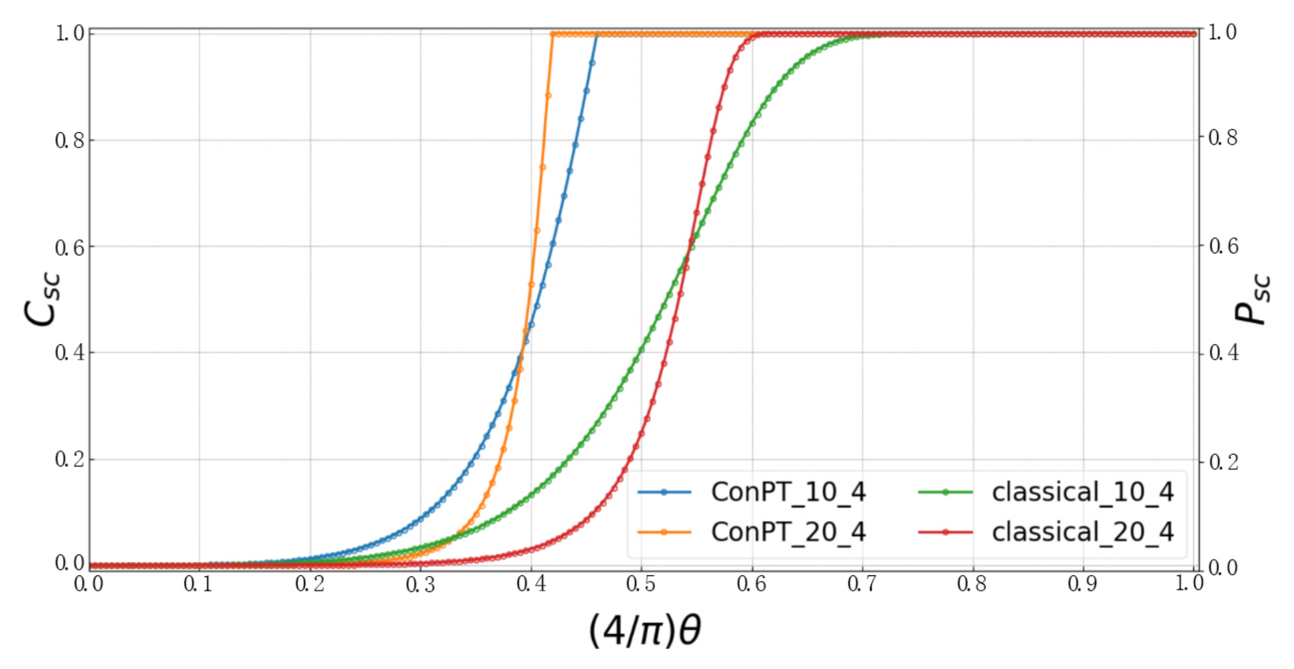
The effect of the average degree on percolation threshold in a WS quantum network is also considered. Take a WS quantum network with an average degree of 4
as an example, as shown in
Figure 12,
. Compared to a WS quantum network with an average degree of 6
:
It can be seen that for WS quantum networks, the percolation threshold obtained after ConPT method has a greater rate of change compared to that after classical method.
For an Erdős–Rényi (ER)) network, an average degree of 6
is selected. By simulation, we can restore the percolation threshold using the classical method
. While using the ConPT method,
is obtained, and the percolation threshold is reduced by
. It is shown in
Figure 13 that the ConPT method can take advantage of concurrency and perform entanglement metric on quantum states to effectively reduce the percolation threshold of the network.


