Evaluation of the Effect of Hamao Detention Pond on Excess Runoff from the Abukuma River in 2019 and Simple Remodeling of the Pond to Increase Its Flood Control Function

Abstract

Due to the recent increase in the intensity of rainstorms, the Japanese government has announced a new policy of flexible flood mitigation measures that presupposes the release of water volumes exceeding the river channel capacity onto floodplains. However, due to the limited amount of quantitative measurement data on excess runoff, it will take time to formulate planning standards for remodeling and newly constructing flood control facilities reasonable enough under current budgetary constraints. In this study, the capacity shortage of a flood detention pond was evaluated against the excess runoff from a severe 2019 flood event by combining the fragmentary measurement data with a numerical flow simulation. Although the numerical model was a rather simple one commonly used for rough estimation of inundation areas in Japan, the results were overall consistent with the observations. Next, in accordance with the new policy, an inexpensive remodeling of the detention basin, which was designed according to conventional standards, was simulated; the upstream side of the surrounding embankment was removed so that excess water flowed up onto the floodplain gradually. Numerical experiments using the simple model indicated that the proposed remodeling increased the effectiveness of flood control remarkably, even for floods greater than the 2019 flood, without much inundation damage to upstream villages.

1. Introduction

In recent years, runoff that exceeds the design capacity of river channels (hereafter referred to as excess runoff) has been increasing in Japan, causing enormous loss of life and damage to assets [1,2,3]. Although its occurrence is still local and infrequent, from a broader perspective, this trend is thought to be growing rapidly due to rising sea surface temperatures on Japan’s south coast caused by global climate change [4].

Therefore, the Ministry of Land, Infrastructure, Transport and Tourism (MLIT), which is in charge of flood disaster prevention in Japan, announced a new flood control policy in 2020 that recognizes the limitations of conventional river channel improvement efforts. In this policy, MLIT emphasizes the need for flexible disaster mitigation measures by planning for river overflow to floodplains. This policy was named “River Basin Disaster Resilience and Sustainability by All” [5,6].

The basis of the conventional policy is to build embankments to separate the locations of hydraulic infrastructure, such as river channels and detention basins from floodplains, which often contain houses and agricultural land. That is, a clear border is established between the spaces where water exists and where it should not enter. In contrast, the new policy essentially proposes to make these borders flexible or temporarily changeable. In other words, the new policy considers a pragmatic approach for modifying the pattern of flooding, which is unavoidable during excess runoff events, in light of the topography and the current state of land use of individual basins, to reduce the damage.

However, the framework for formulating facility design standards based on this policy has not yet been established, and in addition, the investment in flood prevention facilities based on the conventional policy over the past half-century has been very large. Therefore, MLIT is going to continue investing in conventional river improvement works for the time being, that is, for at least the next 10 years [7]. Therefore, during that period, it is important to consider the criteria for facility design based on the new policy as well as the possibility of remodeling existing facilities to meet the new policy.

To clarify the premise for discussing these issues, we first briefly describe the historical process leading to the above-mentioned change in Japan’s flood control policy and the characteristics of floodplains in river basins in Japan, and then, we propose a vision for possible facilities that may meet the new policy. Next, in line with the image of the new type of facility, we will describe the trial design and numerical evaluation of facility remodeling in a river watershed where an excessive runoff has recently occurred.

The site of the case study is a detention pond located in the upstream reach of the Abukuma River, which flows through the northeastern part of Japan’s main island. Excess runoff caused many serious disasters along this river in 2019 [2]. This detention pond is within a rural area located upstream of the city that received the most severe river overflow. There are three reasons for studying it. First, to mitigate flood disasters, runoff control by the intentional inundation of upstream rural areas will be more effective than taking measures in the affected urban areas. Second, although a flood detention pond was constructed in this basin about 20 years ago following the current design standard, this pond was unable to control the excess runoff in 2019. Third, the accidental river overflow in this basin did not cause any serious damage because the land use in that local community followed traditional siting customs that mitigated the impact of flooding.

This case study is purely practical, in that it employs a conventional numerical model that is commonly used in river administration works in Japan [8], and in this sense, it is far from a typical academic study. However, it is hoped that the visualization of today’s issues regarding flood control by a simple approach leads to the development of advanced scientific approaches to the issue. For this reason, in this paper, an overview of the 2019 excess runoff and river overflow at the study site is first given based on the field observation data. Next, numerical simulation is carried out for inundation of the floodplain, as well as the flood control effects of the detention pond, and its consistency with the observed data is verified. Finally, the flood control effect of a trial detention pond remodeled in accordance with the new policy is investigated using the same numerical model. The remodeled detention pond has no surrounding embankment on the upstream side, and thus, when the inflow volume exceeds the storage capacity, the inundated area slowly expands over the upstream floodplain.

2. Current Status of River Management for Flood Prevention and Possible River Improvement by New Policies

2.1. Current Status of Japan’s River Improvements for Flood Prevention

Many of the river embankments in Japan in the early modern period (until the mid-19th century) had openings at key points, and when river flow exceeded the channel capacity, river overflow was intentionally generated. While embankment technology was immature, such river planning was effective in predicting and mitigating flood damage, as well as reducing flood peaks [9,10,11,12,13]. In the latter half of the 19th century, the modern hydraulic control method of promptly discharging floods to the sea by continuous embankments was introduced by European engineers, and a modern river plan was made in 1911 for 13 nationally controlled rivers, as stipulated by the River Law at the time. However, in many other rivers, embankment systems with overflow openings have survived for a long time.

The New River Law, which came into effect in 1964, mandated the formulation of a modern river plan for rivers nationwide. By about 1970, a river improvement master plan was formulated for the 109 nationally controlled water systems, and river channel improvement works were started to safely flow flood discharge downstream as specified in the plan. The annual generation probability of target floods in this plan was set at 1/100 to 1/200 for each river system, based on population concentration and economic importance. However, the master plan did not specify completion deadlines, so necessary expenses are not linked to annual budgetary preparation. The total length of the embankments of Class A rivers, which are directly managed by the national government, is more than 13,000 km. In addition, part of the budget for river improvement works must be spent for restoration after every flood disaster. As a result, the pace of river improvement is still slow.

Therefore, in a report submitted in 2000, the Panel on Social Infrastructure Development concluded that if the construction of a continuous embankment is economically or physically difficult, methods other than the continuous embankment, including floodplain countermeasures, should be considered. In addition, to clarify the step-by-step procedure and progress evaluation, the River Law was partially revised in 2005 to prepare a river improvement plan for a period of 30 years for each river system. Currently, construction is underway according to the first-stage river improvement plan, which will be completed around 2035.

The blue dots in Figure 1 show the correlation between the river channel flow capacity targeted in the first river improvement plan (hereafter referred to as “current channel capacity”) and the flood discharge specified in the master plan at the river management reference point. The orange dots are the correlation with the river discharge expected after the flood control by dams and detention basins shown in the master plan (planned high-water flow rate), although many of them are still just planned or under construction. Therefore, even after the completion of the first-stage river improvement, a considerable amount of river channel improvement and flood control facility construction are required.

Moreover, in light of the frequent increase in torrential rains in recent years, the MLIT has performed numerical long-term climate simulation and announced that the flood flow rate specified in the master plan must be increased by at least 1.2-fold to meet the annual probability of target floods under future climate change [14]. However, considering the progress of current river improvement projects, even if the target flow rate is increased, it will take a tremendous amount of time to achieve it. In other words, only reforming the master plan does not actually improve protection from flood disasters.

Figure 2 shows the relationship between the ratio of extreme flood discharge and that of the annual frequency of occurrence by a sample analysis. The decrease in the return period corresponding to the ratio of the current target flow rate (1:1.2) to the target flow rate of the future master plan indicated by the double circle is about 50%. In other words, the frequency of river flooding will double. For example, a flood with an annual probability of 1/100 in the current master plan will be 1/50 in the future. In view of the above situation, it was considered more effective to switch to a flood disaster prevention strategy that allows flooding once every 50 years (for example), rather than continuing river improvement according to the master plan. This was the reason why the new policy, “River Basin Disaster Resilience and Sustainability by All” was announced in 2020.

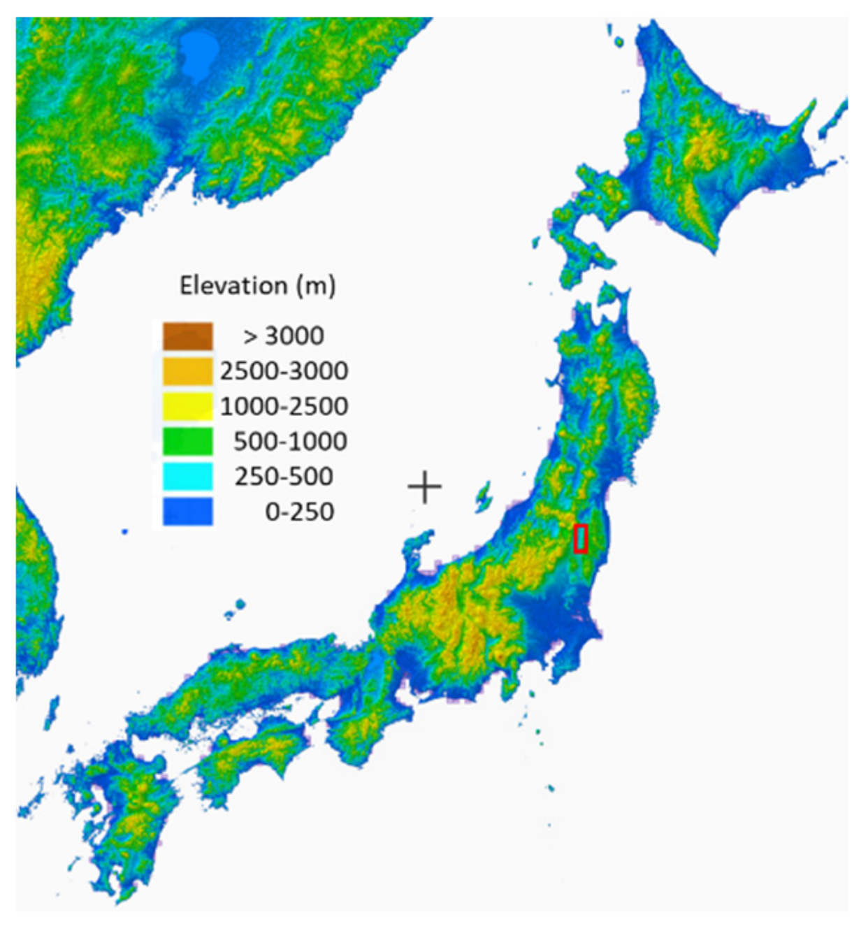
2.2. Topographical Features of the Upper Reaches of Rivers in Japan

To specifically plan river overflow in accordance with the new policy, attention must be paid to the topographical features of the floodplain. Here, the characteristics typical of a Japanese river floodplain are explained using the Abukuma River, which is the site of this study, as an example. As shown in Figure 3, 70% of Japan’s land area is mountainous, with rivers flowing through the narrow valleys between them. Figure 4 is the “landform classification map for flood control [15]” of the upper reaches of the Abukuma River, which is surrounded by a red frame in Figure 3. This type of map shows the classification of the microtopography formed by river floods, such as floodplains, natural levees, and old river tracks. In the valley bottom plain, small basins and constrictions are connected in series, and it can be seen that the meandering river channel often touches the hill edges (hereafter referred to as “hill corners”). Due to these topographical features, until recently, floodplains (yellowish green) in the basins were temporarily flooded during deluges and had the flood control effect of reducing the peak discharge. However, by the continuous levees (black lines with scales) built monotonously according to the conventional river improvement policy, the flood retarding effect was lost, and the peak of the downstream flood increased.

Figure 5 is an enlarged view of the area outlined by the red rectangle in Figure 4. The pink dots indicate the distribution of houses. Most of the houses are on plateaus that are unaffected by river floods and on natural levees that are less frequently flooded. The floodplains mostly comprise paddy fields, with almost no houses. In other words, for a long time, land use has been based on the expectation of river flooding.

There are three basin terrains in the figure; for convenience, they are called the first, second, and third basins from the upstream direction hereafter. The Hamao Detention Pond (HDP), which is described in detail in Section 3.2, is located in the third basin. The river section directly managed by the national government extends up to the second basin, where continuous levees have been constructed. In contrast, the river channel of the first basin is managed by the Fukushima prefecture, and the embankment remains unfinished (brown in the figure) due to the restrictions of the prefecture’s budget.

A closer look at the shape of these unfinished embankments reveals that they are open upstream of the hill corners, as marked by the three red open arrows. Until the 1970s, such levee openings existed in the upper reaches of many rivers in Japan, but they gradually disappeared as continuous levees were extended from downstream [16]. Old river tracks and drainage channels were connected to such levee openings and were used for drainage after the paddy fields on floodplains were inundated. In addition, as shown in Figure 6, it is probable that floodwaters from the opening gradually spread upstream during the large flood, which contributed to the reduction of the flood peak.

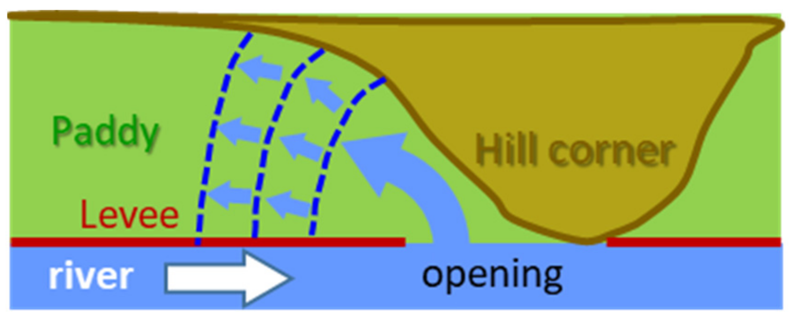
2.3. Expandable Detention Pond That Uses Natural Terrain

In the early modern times of Japan, flood control by intentional river overflow from levee openings was commonly adopted, and some openings still exist in upstream river sections, as shown in Figure 6. The authors think that this type of flood control facility, which was common in the past when flood discharge frequently exceeded the river channel capacity, gives hints for facility design under the new policy of the MLIT. However, simple levee openings will cause frequent damage to agricultural land. Thus, we considered a detention pond against excess runoff, as shown in Figure 7.

When a continuous levee is constructed, a gutter gate is usually included at the hill corner for drainage of inundation water on the plain. An overflow dike is installed on the upstream side, and when the river water level exceeds a predetermined level (for example, the planned high-water level [HWL]), the river water enters the plain. Then, the overflowing water gradually spreads to the upstream side, and it is not necessary to install a surrounding embankment because it does not spread indefinitely due to the terrain gradient. After the river water level drops, floodwater is discharged from the gutter gate into the river channel. The construction cost will be much lower than that of a normal detention pond with a surrounding embankment. Because there are many terrains in the upper reaches of rivers in Japan where such facilities can be installed, it is possible that the flood peak of excess runoff will be significantly reduced due to this effect. As mentioned earlier, the HDP located in the third basin shown in Figure 5 did not have the effect of reducing the peak discharge during the excessive runoff in 2019. Thus, we examined the improvement of flood control effect after remodeling the HDP to the form shown in Figure 7.

3. Description of the Study Site

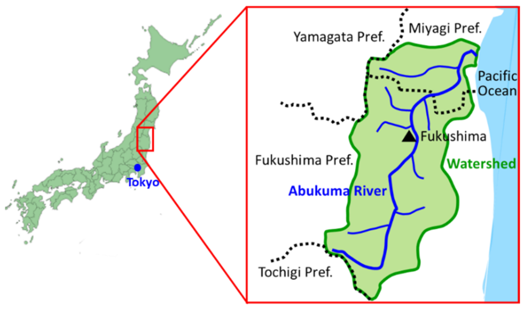
3.1. Overview of the Abukuma River Watershed

The Abukuma River is a nationally managed first-class river that flows northward in the eastern part of Honshu Island with a length of 239 km and watershed area of 5390 km² (see Figure 8). The downstream section of 49 km and the upstream section of 190 km belong to Miyagi and Fukushima prefectures, respectively. Figure 9 shows the longitudinal distribution of the progress of river improvement projects currently underway. The top of the red vertical arrow shows the forecast for 2035, when the project will be completed. The expected completion level in Fukushima, the river management reference point, is 80% but it is about 60% in the upstream area.

The record of the annual maximum flow rate in Fukushima shown in Figure 10 indicates a tendency of increased flooding over time. The target flood scale for river improvement works set in 1964 is 150 years in the return period, and the corresponding river channel capacity necessary for flood prevention at the Fukushima reference point is a flow rate of 5800 m³/s. Toward this goal, river improvement work has been ongoing for about 60 years, and it is expected that a river channel capacity of 4600 m³/s will be achieved by 2030. However, the maximum discharge in 2019 exceeded 6000 m³/s.

The recent largest flood before 2019 occurred in 1998, and a large-scale upstream river improvement project was carried out based on the flood data obtained at that time. As part of this project, the Hamao Reservoir (HDP) was constructed at the location shown in Figure 5 in 2005. Figure 11 compares aerial photographs before and after construction. Prior to the construction of the HDP, the river channel was straightened and enlarged.

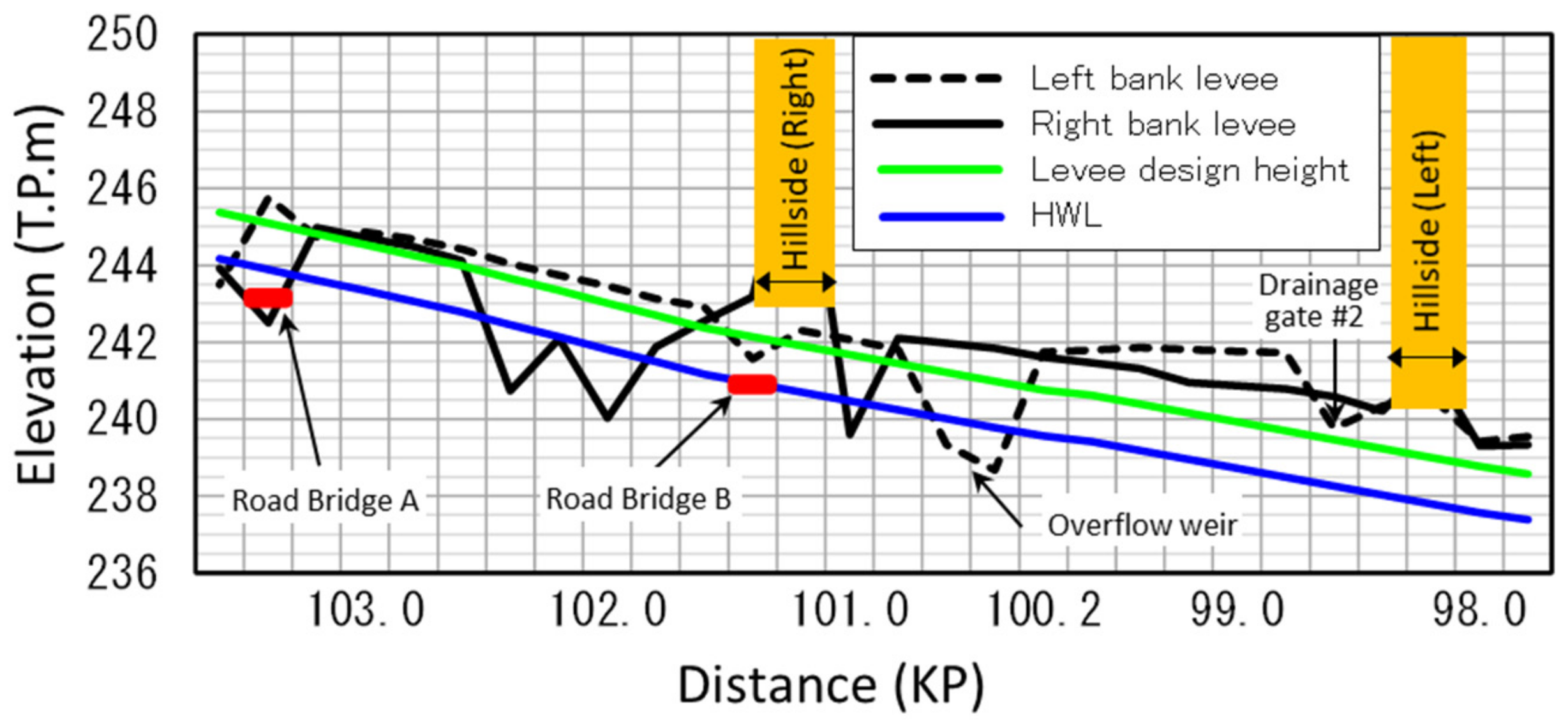
3.2. Terrain and Hydraulic Facilities of the HDP

Figure 12a,b shows an enlarged map of the basin terrain and structure of the HDP, respectively, in which KP indicates the river channel distance from the Miyagi–Fukushima prefectural border. The HDP is located near the exit of the basin of about 300 ha, and it has an area of 62 ha and storage capacity of 1,800,000 m³/s. The intricate part of the river trace near the HDP corresponds to the old river channels straightened in the early 2000s. Natural levees are widely developed on the left bank upstream of the HDP, and the central part of the basin is classified as a floodplain. This means that the river often overflowed onto the floodplains before the levee was constructed for channel improvement.

Figure 13 shows the elevation of the floodplain along the survey line (C-C’) indicated in Figure 12a. The HDP was partially excavated from the original ground level to create the required storage capacity. The basin terrain has a slope of about 1/500. Figure 14 shows a longitudinal view of the left and right banks, as well as the planned HWL. The levee design height (green line) is the HWL plus the freeboard stipulated by the structural ordinance for river facilities [9]. The levee further has an extra height of about 50 cm in anticipation of future land subsidence.

The top of the left levee from 98.8 to 100.2 KP is horizontal because it also serves as an enclosure levee for the detention pond. At 98.6 KP, there is a gate for draining local runoff (hereafter referred to as the second drainage gate), and the levee does not have additional height at this location. The top of the left levee around 101.4 KP and 103.4 KP is lower because road bridges that predate the levee construction are present. The right levee from 101.6 to 102.4 KP was not completed at the time of the 2019 flood and was lower than the design height.

In this area, as indicated by colored triangles in Figure 12a, observation facilities are located at many positions. Two water level observatories (indicated by red triangles), named Sukagawa and Kosakuda, are located near the exit and the entrance of the basin terrain. At the time of the flood, in addition, the flow rate was estimated from the velocity measurement using a float thrown into the river from the bridge. However, for the 2019 flood, data are not available from the Kosakuda Observatory because the water gauge was damaged by submergence.

Water gauges are also installed on the land side of two drainage gates (indicated by green triangles), which were built inside and outside of the HDP. Because flooding was anticipated from the locations of the two road bridges upstream of the HDP (indicated by blue triangles), temporary water gauges, named 3 L water gauges [17] have been installed on the bridges to measure the water levels only during floods.

The solid blue line in Figure 15 shows the relationship between the water level and the storage capacity of the HDP. As currently configured, the inflow begins when the river channel water level exceeds 238.35 T.P.m. Here, the T.P.m is the elevation in meter measured from the average tide level in Tokyo Bay. The top of the surrounding embankment is at 241.7 T.P.m. In contrast, the solid red line shows the relationship where the surrounding embankment of the detention pond is removed. This is explained in Section 7. Figure 16 shows the estimated results of the flood control effect on the 1998 flood. A peak reduction of about 90 m³/s is shown. The peak flow rate of this flood is about 70% of the high-water flow rate written in the master plan, and the probability of occurrence is estimated from Figure 2 to be about 45 years. The reason for not using the master plan hydrograph in the design of the HDP was probably that the downstream river channel was still far smaller than that in the master plan. In other words, the HDP was designed to respond immediately to the recently experienced flooding rather than as a part of the master plan.

4. Overview of the Large Flood in 2019

River overflow occurred at the three locations indicated by thick red arrows in Figure 17: two locations on the left bank at the two old bridges (A and B) and one long stretch of the right bank where the levee construction was incomplete (C). In addition, because the second drainage gate downstream from the HDP was open until near the peak of the flood, river water reached the upstream side of the levee surrounding the HDP. After that, the gate was closed, but because the river water flowed from the two old bridges down to the second drainage gate, the levee above the gate was overtopped, and the gate broke after the water level in the channel declined [18]. This location is marked by the double-headed arrow (D) in Figure 17.

Figure 18a shows the observation records of water level and flow rate at the Sukagawa Observatory. The T on the horizontal axis is the elapsed time from 12:00 on 12 October 2019. The red dotted curve is the flow rate obtained from an interpolation using the correlation diagram of water level and flow rate depicted in Figure 18b. The water level reached the HWL around T = 10:00 and peaked around T = 19:00. The highest water level exceeded the HWL by more than 1.5 m and just reached the top of the embankment. Figure 19 shows the observed water levels at the other points together. Measurements at the two upstream road bridges were taken only during the time when the water level was overflowing the embankment, and measurement on the land side of the drainage gates #1 and #2 the location of which were shown in Figure 12b stopped before the flood peak due to submergence of the measuring instrument. In addition to these data, the river channel trace water level was measured after flooding, which showed that the highest water level exceeded not only the HWL, but also the levee design height over the entire section, as discussed in more detail in Section 6. The data described above are listed in

Table 1. Locations and durations of hydrological measurements for the 2019 Abukuma flood.

Measurement Point	Symbol	Measurement Duration	Elapsed Time
Sukagawa (water level)	$H_{S0}$	12th 12:00–14th 0:00	0:00–36:00
Sukagawa (flow rate)	$Q_{S0}$	12th 12:00–14th 0:00	0:00–36:00
Road bridge A	$H_A$	12th 23:00–13th 11:50	11:00–23:50
Road bridge B	$H_B$	12th 23:00–13th 11:50	11:00–23:50
Discharge gate #1	$H_{\mathrm{H}}$	12th 17:00–13th 0:50	5:00–12:50
Discharge gate #2	$H_{\mathrm{D}}$	12th 17:30–13th 2:30	5:30–14:30
River channel (flood peak trace)	$–$	After flood	$–$

.

As shown in Figure 10, because the 2019 flood was of an extraordinary scale that had not been recorded previously, complete observation data were not obtained due to observation equipment failures. In the next section, the above fragmentary data are supplemented with numerical simulation to provide an overall picture of the flood.

5. Methodology for Flood Analysis

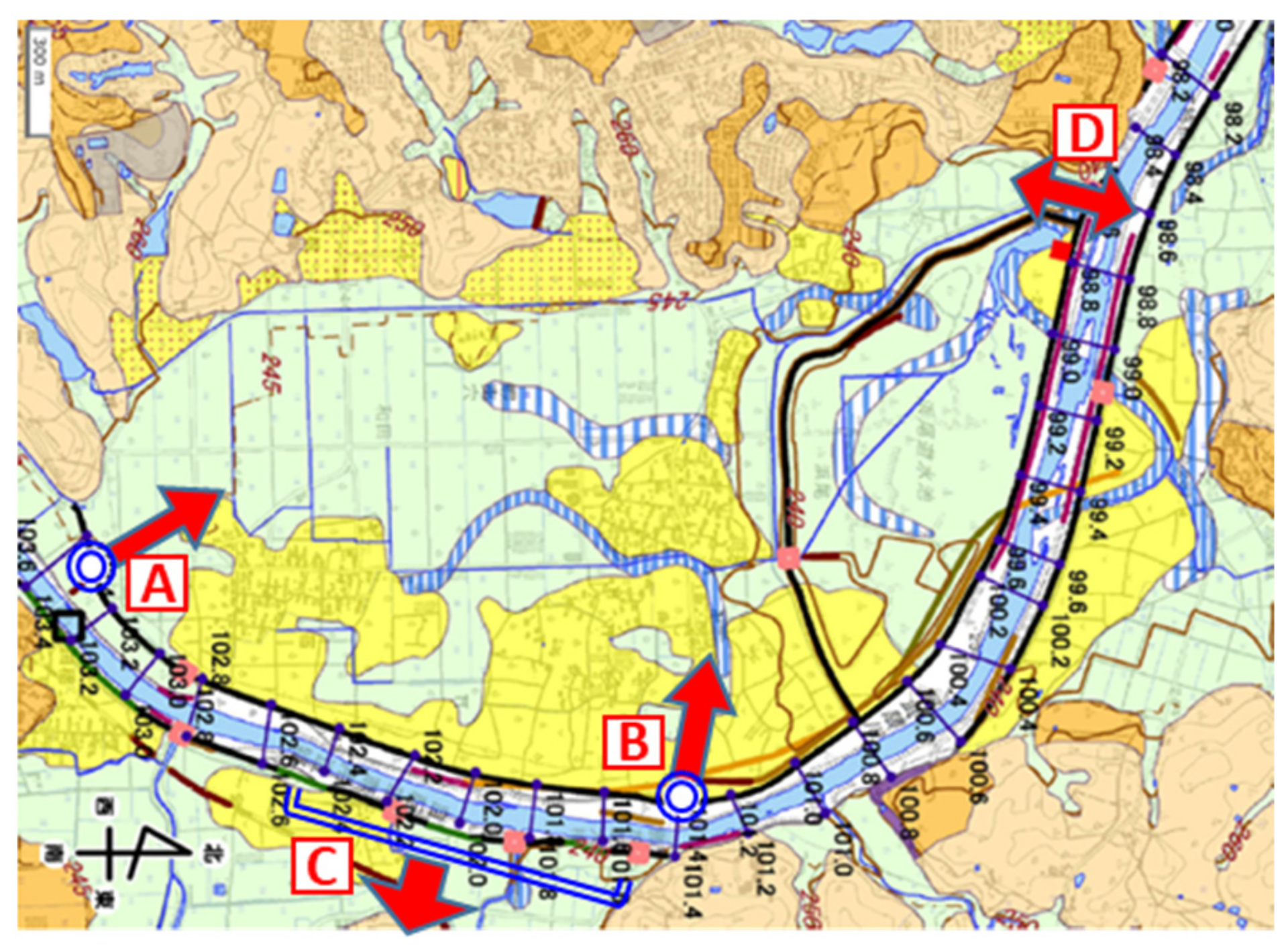
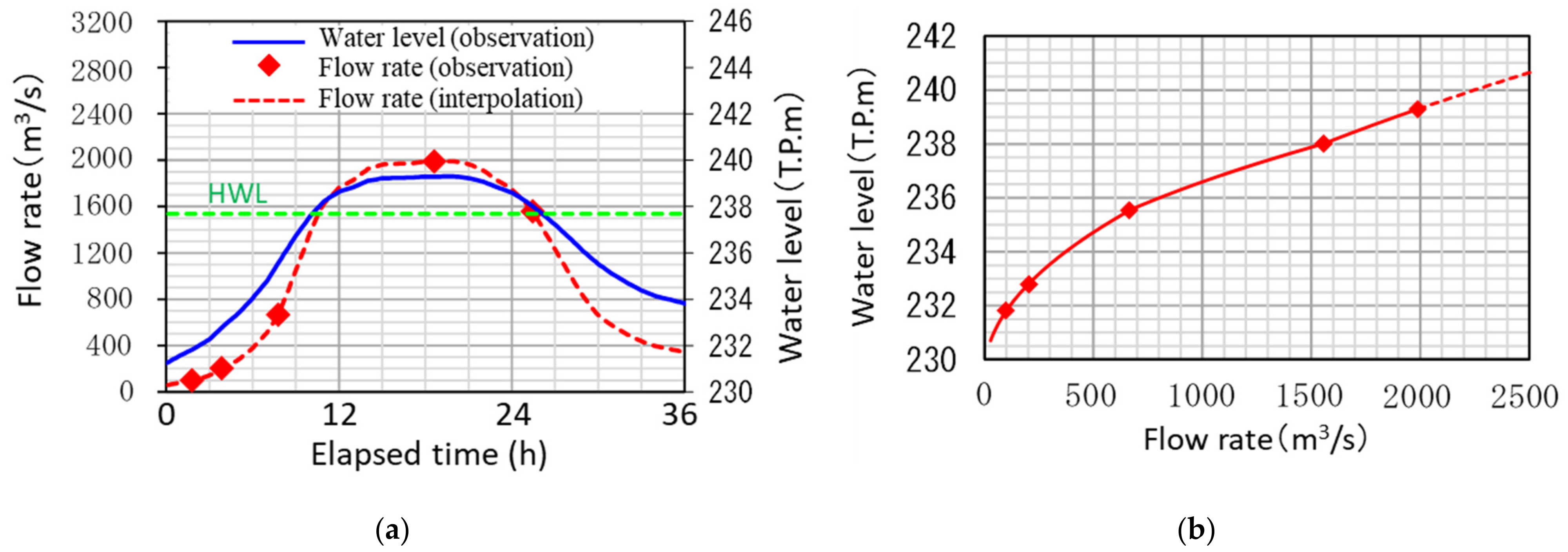
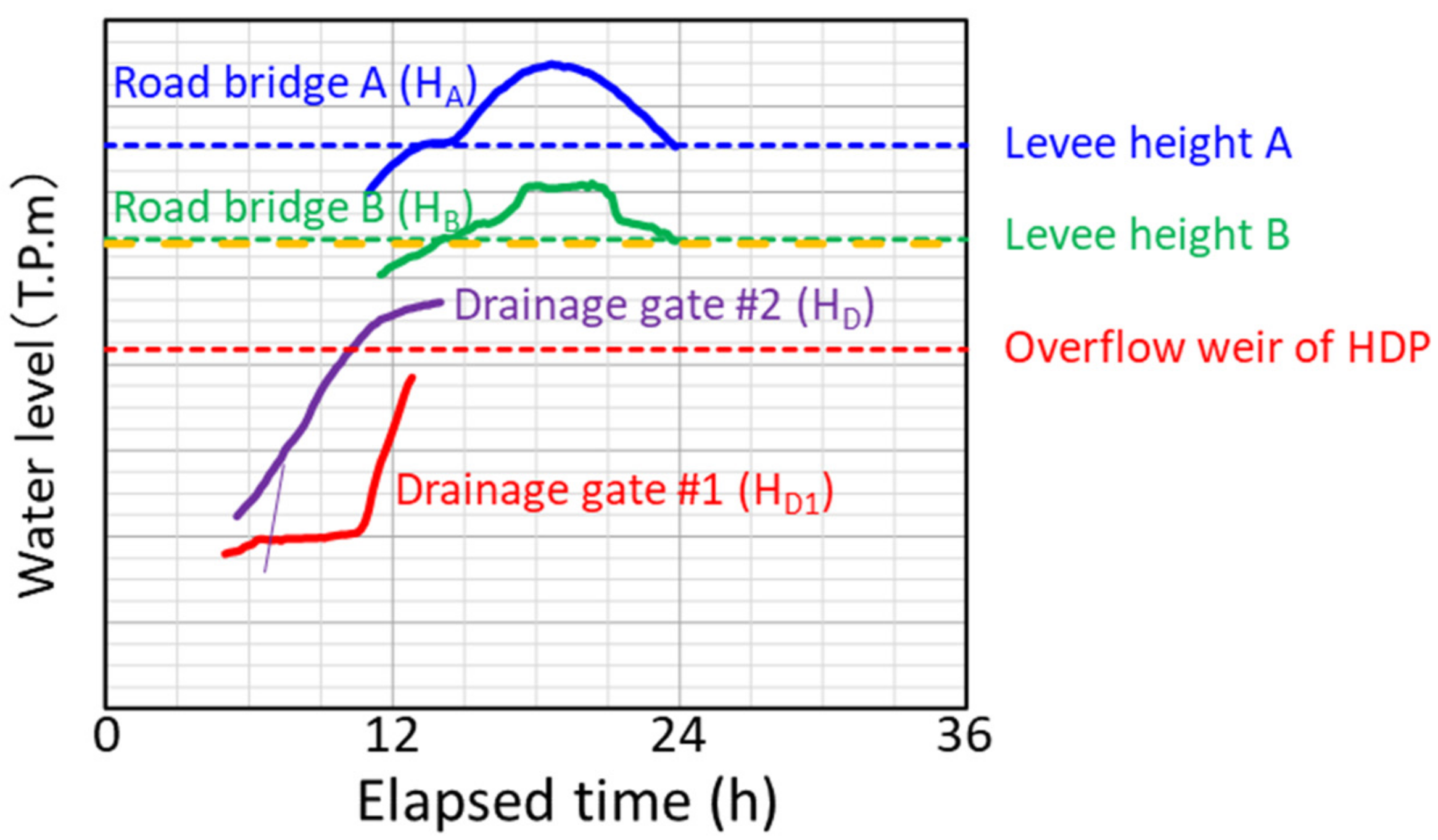
5.1. Estimation of River Overflow Pattern from Water Level Data

Figure 20 schematically illustrates the river channel and floodplain flow fields in 2019. The blue arrow in the center indicates the river channel, the yellow areas on the two sides indicate the floodplains, and the light blue section indicates the HDP. The arrows ($q_A, q_B, \mathrm{and} q_C$) from the river channel to the floodplain indicate the river overflow, and the double-headed arrow ($q_H$) indicates the water exchange between the river channel and the HDP. Two arrows ($q_D \mathrm{and} q_E$) in different directions are plotted separately on the second drainage gate near the downstream end, the former indicating the flooding when the gate was open and the latter indicating the levee overtopping from the land side after the gate was closed.

It is not easy to simulate a complex flow field containing such a large number of branches with a single numerical model. Therefore, prior to the analysis of the entire flow field, some variables were estimated in advance from the measurement data.

5.1.1. Rate of River Overflow Flow at Points A and B

At the two points where river overflow occurred due to the existence of old road bridges indicated with A and B, the river water level record during the flood by 3 L water gauges was obtained (see $H_A$ and $H_B$ in Figure 9). Therefore, the overflow rate was calculated using the formula describing the relation between flow rate and overflow depth proposed by [19], and the calculation results were used in the simulation of the entire flow field.

$$q=\left\{\begin{array}{c}0.35 h_1\sqrt{2g{h}_1} \mathrm{when} \frac{h_2}{h_1}\le \frac{2}{3}\\ 0.91 h_2\sqrt{2g\left(h_1-h_2\right)} \mathrm{otherwise},\end{array}\right.,$$

(1)

where $h_1$ and $h_2$ are the water level on the two sides measured from the levee top ($h_1>h_2$) and $q$ is the flow rate per unit width on the embankment.

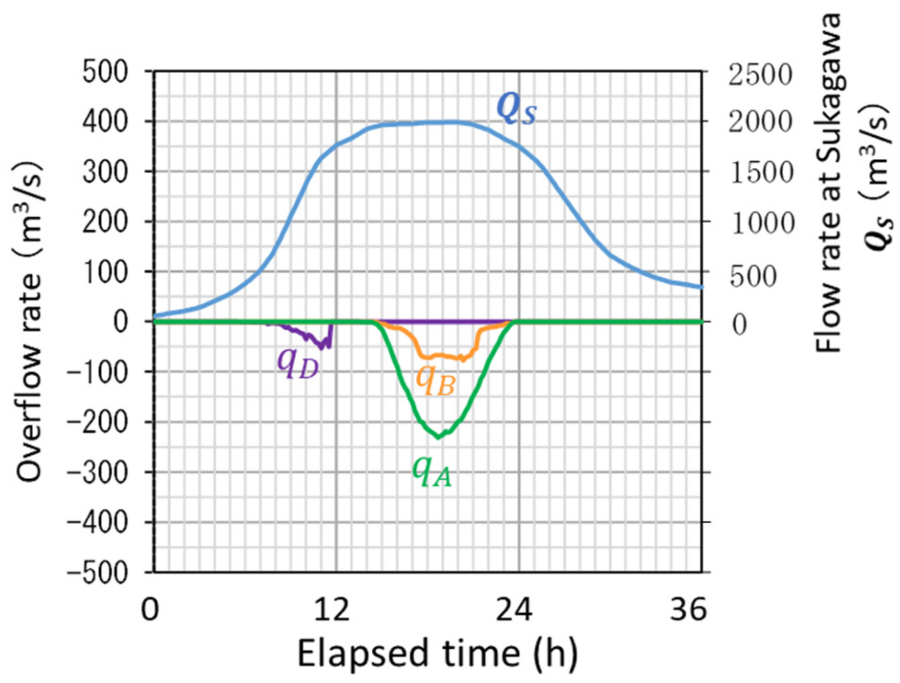
5.1.2. Backward Flow Rate from the Second Drainage Gate

Because the second drainage gate was still open when the river water level was still rising, the river water intruded backward into the downstream end of the floodplain through the gate, and the inundation slowly expanded upstream against topographical gradient. Until the gate was closed, the water level was recorded by a water gauge installed on the land side (see $H_D$ in Figure 19). Because the water surface of the slow reverse flow was almost horizontal, the flow rate, $q_D$, was calculated from the following volume conservation equation:

$$q_D\left(t\right)=\frac{d}{dt}\left({{\displaystyle \int }}_{z_0}^{H_D\left(t\right)}A\left(\zeta \right)d\zeta \right),$$

(2)

where $\zeta$ is the vertical coordinate taken upward from some datum level, and $A\left(\zeta \right)$ is the area of the water surface at height $\zeta$.

The overflow rate ($q_A, q_B, q_D$) calculated based on the above assumptions is shown in Figure 21 together with the observed flow rate at Sukagawa. It can be seen that they are about 10% of the river channel flow rate at the maximum. The remaining overflow rates ($q_C, q_H, q_E$) were obtained in a flow simulation using the numerical model described below.

5.2. Numerical Model for Flow Field Analysis

The numerical model adopted in this study uses a one-dimensional unsteady flow equation for the river channel and a set of shallow-water flow equations on a rectangular grid system for the floodplain, and it connects the two based on Equation (1) to express the total flow system [7].

Because the river overflow rates to the left floodplain ($q_A, q_B,q_D$) were determined in advance, as shown in Figure 21, the flow field on the left floodplain was simulated independently from the river flow calculation. Manning’s roughness coefficient was set to 0.04, which is recommended for paddy fields in Japan. Figure 22 shows the spatial distribution of the calculated maximum inundation depth, as well as the outer edge of the inundation area obtained from the inundation trace survey conducted by MLIT Fukushima Office of Rivers and National Highways after the flood. The results show a good match between them.

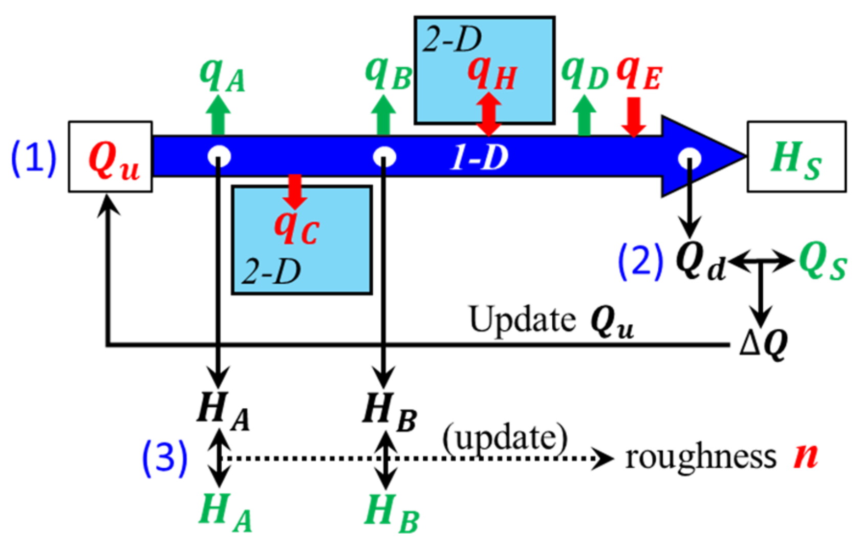
5.3. Iterative Calculation Method to Obtain the Entire Flow Field

As discussed in Section 4, due to damage to the water gauge at the Kosakuda Observatory during the 2019 flood, the hydrograph data at the upstream end of the calculation are not known. In addition, because floods of this magnitude were unprecedented, the corresponding river channel roughness coefficient is also unknown. Therefore, an iterative procedure was adopted, as described in Figure 23.

In the figure, the thick blue arrow represents the river channel, and the vertical arrows represent the water exchange between the river channel and floodplains or between the river channel and the HDP. The variables expressed as green symbols were determined in advance from the observation data, the red symbols are the variables that were determined by the iterative calculation, and the black symbols are the variables that are intermediate results during the iterative calculation. The meanings of $q_A, q_B, q_C, q_D, q_E$ and $q_H$ are the same as those given in Figure 20. The water level at the downstream end of the calculation is equal to the observed water level at Sukagawa, $H_S$ (see Figure 18a). $Q_u$ and $Q_d$ are the river channel discharges at the upstream and downstream ends, respectively, the latter of which must eventually converge to the discharges observed at the Sukagawa Observatory, $Q_S$ (see Figure 18a). $H_A$ and $H_B$ are the water levels at the points of the old road bridges where the 3 L water gauges were installed, and they must eventually converge to the observed records. The variable n is the roughness coefficient of the river channel, which is determined in reference to the observed water levels at points A and B, as well as the longitudinal profile of the highest water level.

The iteration procedure was as follows. Steps (1), (2), and (3) below correspond to the numbers shown in blue in Figure 23.

(1)

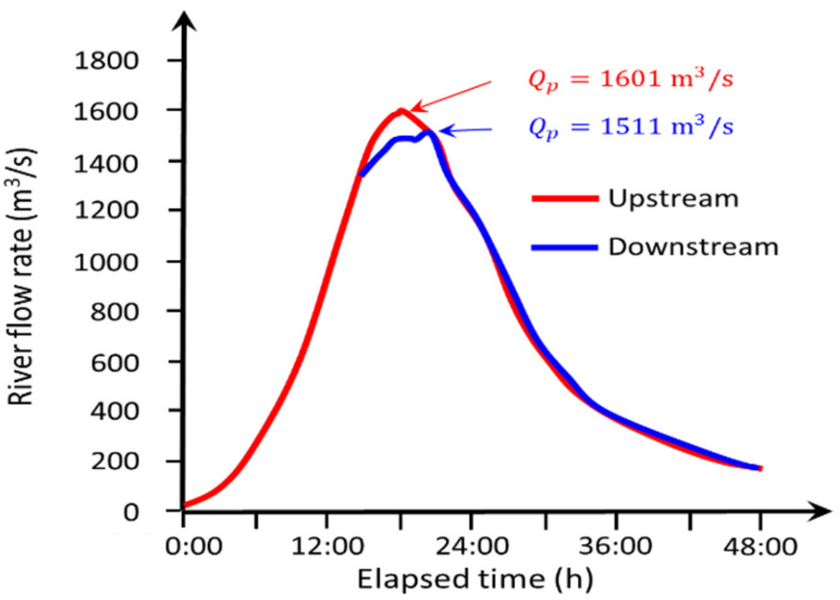
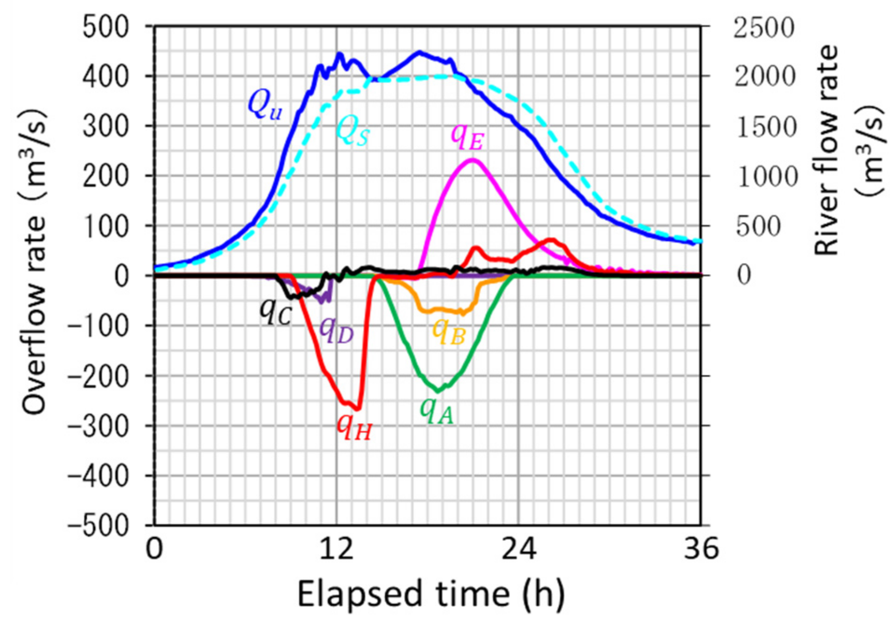
First, an appropriate $Q_u\left(t\right)$ for the upstream end boundary condition is assumed, and the downstream boundary condition $H_S\left(t\right)$ is set to perform a one-dimensional unsteady flow analysis considering the water exchange with the floodplain and the HDP. In this calculation, $q_A\left(t\right), q_B\left(t\right), \mathrm{and} q_D\left(t\right)$ are given as the hydrographs shown in Figure 21, while the unknown variables $q_C\left(t\right), q_H\left(t\right), \mathrm{and} q_E\left(t\right)$ are calculated using Equation (1).

(2)

The downstream end flow rate $Q_d\left(t\right)$ obtained by the calculation is compared with the Sukagawa observed flow rate $Q_S\left(t\right)$, and the upstream flow rate is updated by subtracting their difference $\Delta Q\left(t-\Delta t\right)$ from the $Q_u\left(t\right)$, in which $\Delta t$ is the time for floodwater to reach the downstream end from the upstream end.

(3)

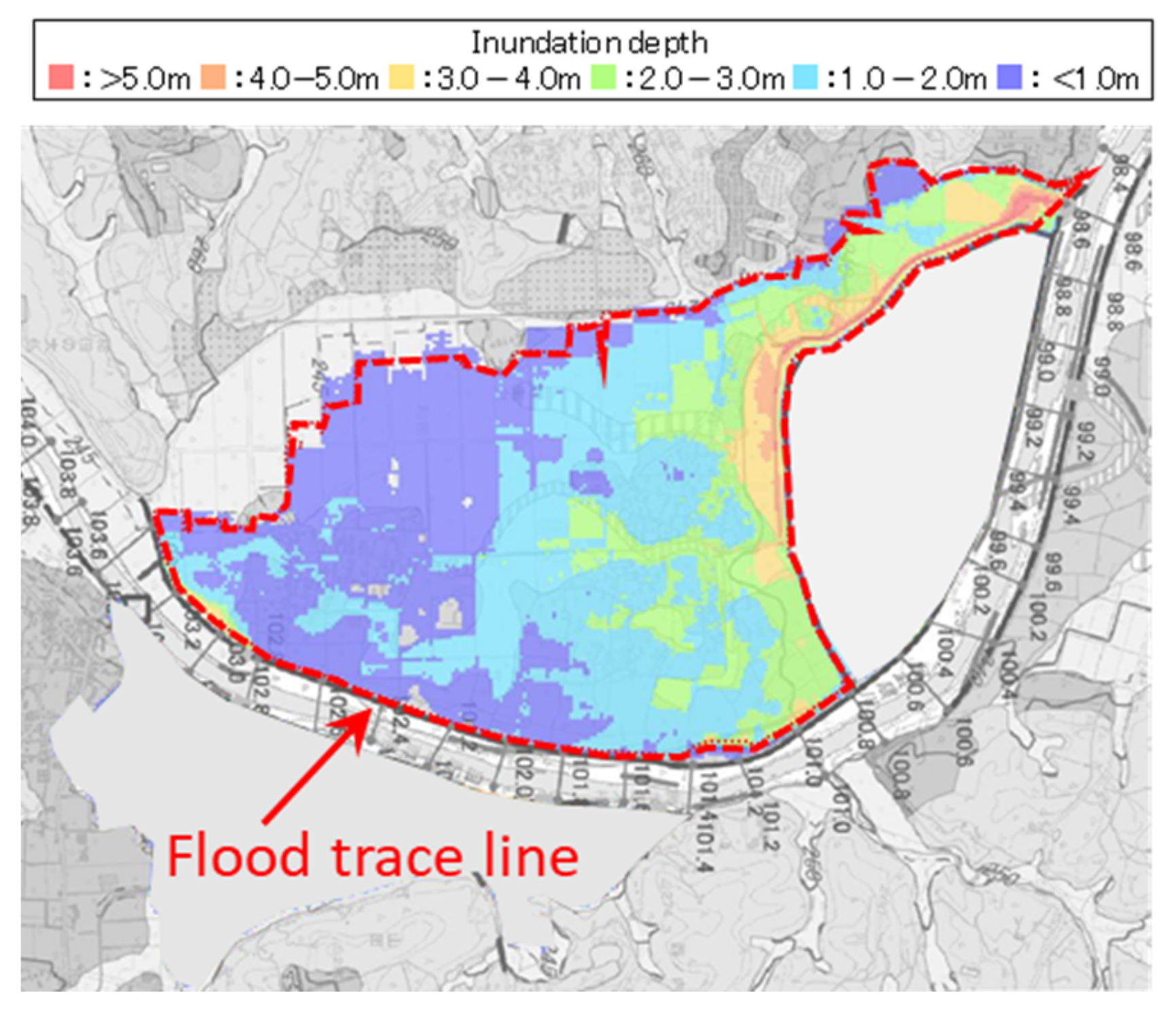
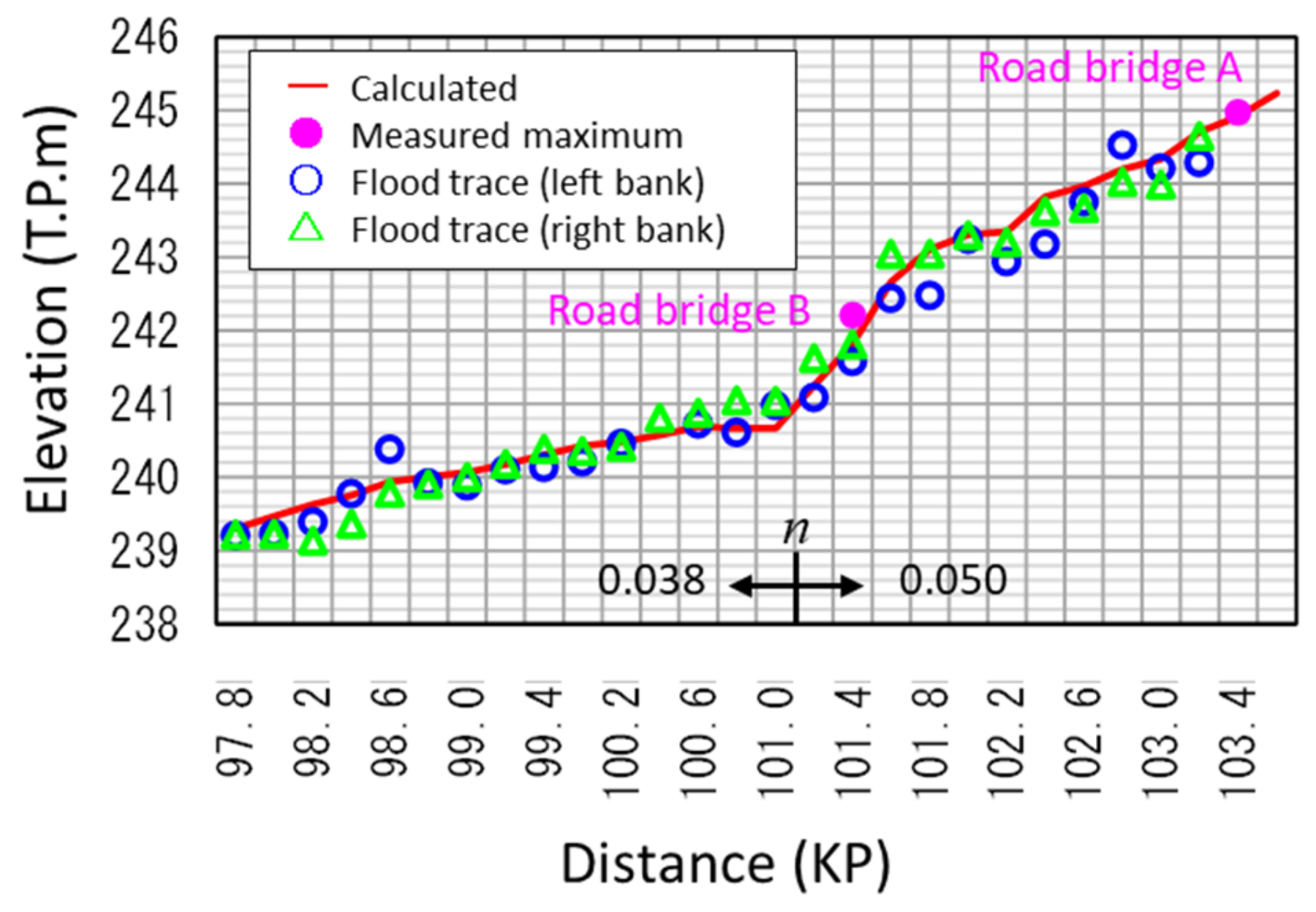
Manning’s roughness coefficient, $n$, is updated with reference to $H_A\left(t\right)$ and $H_B\left(t\right)$ obtained by the 3 L water gauges, and the longitudinal distribution of the highest water level obtained from the flood traces.

First, $q_C\left(t\right), q_H\left(t\right), \mathrm{and} q_E\left(t\right)$ were set to zero, and $Q_u\left(t\right)$ was assumed as the following equation to perform preliminary calculations to determine ∆ t.

$$Q_u\left(t\right)\Leftarrow Q_S\left(t\right)+q_A\left(t\right)+q_B\left(t\right)+q_D\left(t\right).$$

(3)

Figure 24 compares the calculated downstream end flow rate and the Sukagawa Observatory flow rate. Because there is a time difference of about 30 min, we fixed $\Delta t$ to this value in subsequent iterative calculations.

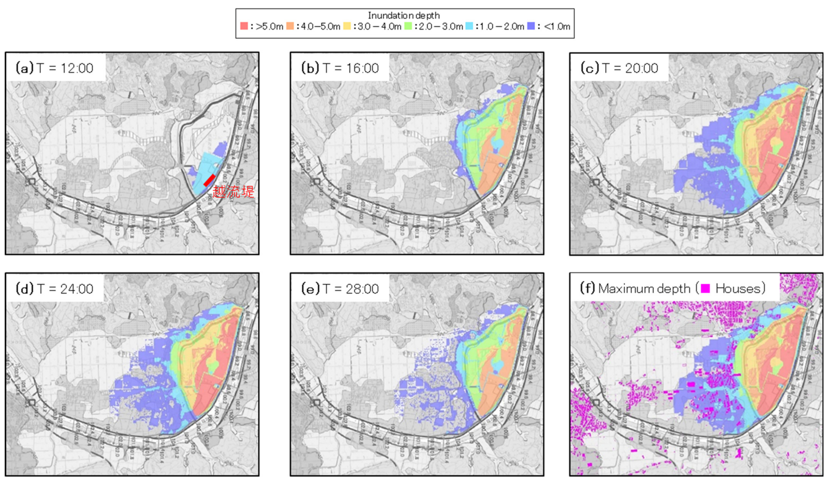
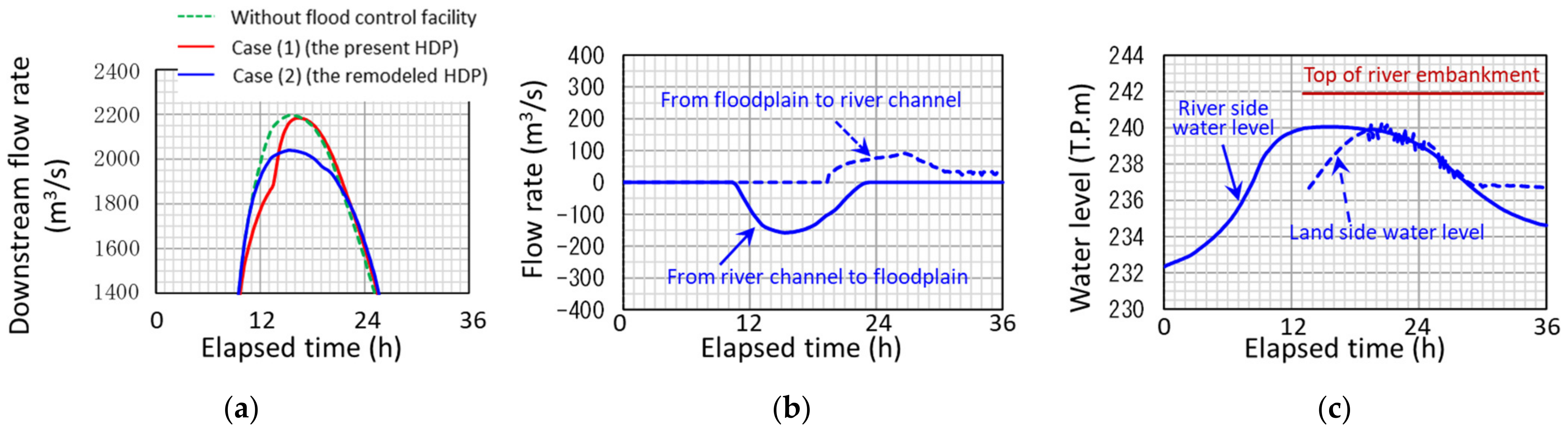
6. Numerical Simulation Results

Figure 25a,b shows the states of convergence of flow rates at the downstream end the upstream end, respectively. It can be seen that $Q_d\left(t\right)$ converged to $Q_S\left(t\right)$ with three iterative calculations. Figure 26 shows the longitudinal profile of the calculated maximum water level of the third iteration, along with the flood traces and the maximum water level measured by the water gauges installed at points A and B. The final value of Manning’s roughness is also indicated in the figure.

Figure 27 shows the temporal changes in the inundation area and in the inundation depth distribution: (a) inundation began from part of the low levee on the right bank, (b) inflow to the HDP started, (c) the HDP filled before the flood peaked, (d) inundation to the left bank side floodplain started, and (e) the inundation flow from upstream arrived at the second drainage gate.

Figure 28 shows the calculation results of the water level at the second drainage gate at the most downstream end of the floodplain. The arrows above the curve reflect events reported by the River Administration Bureau based on a video taken by neighboring citizens and the gate operation record. The black dotted curve is the water level record on the land side of the gate, and the blue curve is the calculated water level. Before the gate was closed around 12:00, the observed water level rose due to the inflow from the river, and the record stopped then due to the submergence of the water level gauge. The water level became stationary after the gate closed, but it rose rapidly at around 17:00 because flow arrived from the upstream floodplain. Around 18:00, levee overtopping began from the land side toward the river channel, and the embankment above the water gate collapsed around 24:00. The calculated water level variation agreed with the recorded events fairly well.

Figure 29 shows the time variation of each overflow component ($q_A, q_B, q_C, q_H, q_{ D}, \mathrm{and} q_E$) together with the river flow rate at the upstream and downstream ends (note the difference in scale on the vertical axes). The inflow into the HDP, $q_H$, ended in the first half of the flood and did not contribute to the lower level of the second flood peak. Instead, the overflow from upstream point A reduced the second flow peak effectively. This inundation flow arrived at the second drainage gate 2 h later, and the embankment above the drainage gate was broken by overtopping, as shown in Figure 28.

The numerical simulation results described above show good overall agreement with the observations.

7. Considerations for Remodeling the HDP to Improve Flood Control Capability

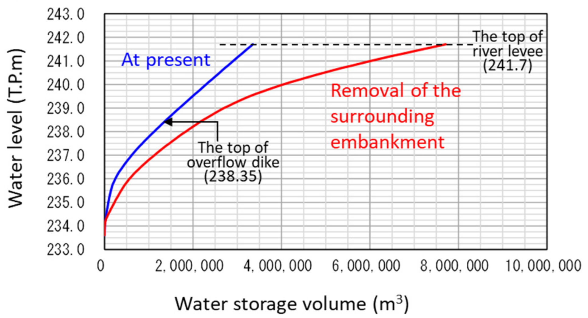
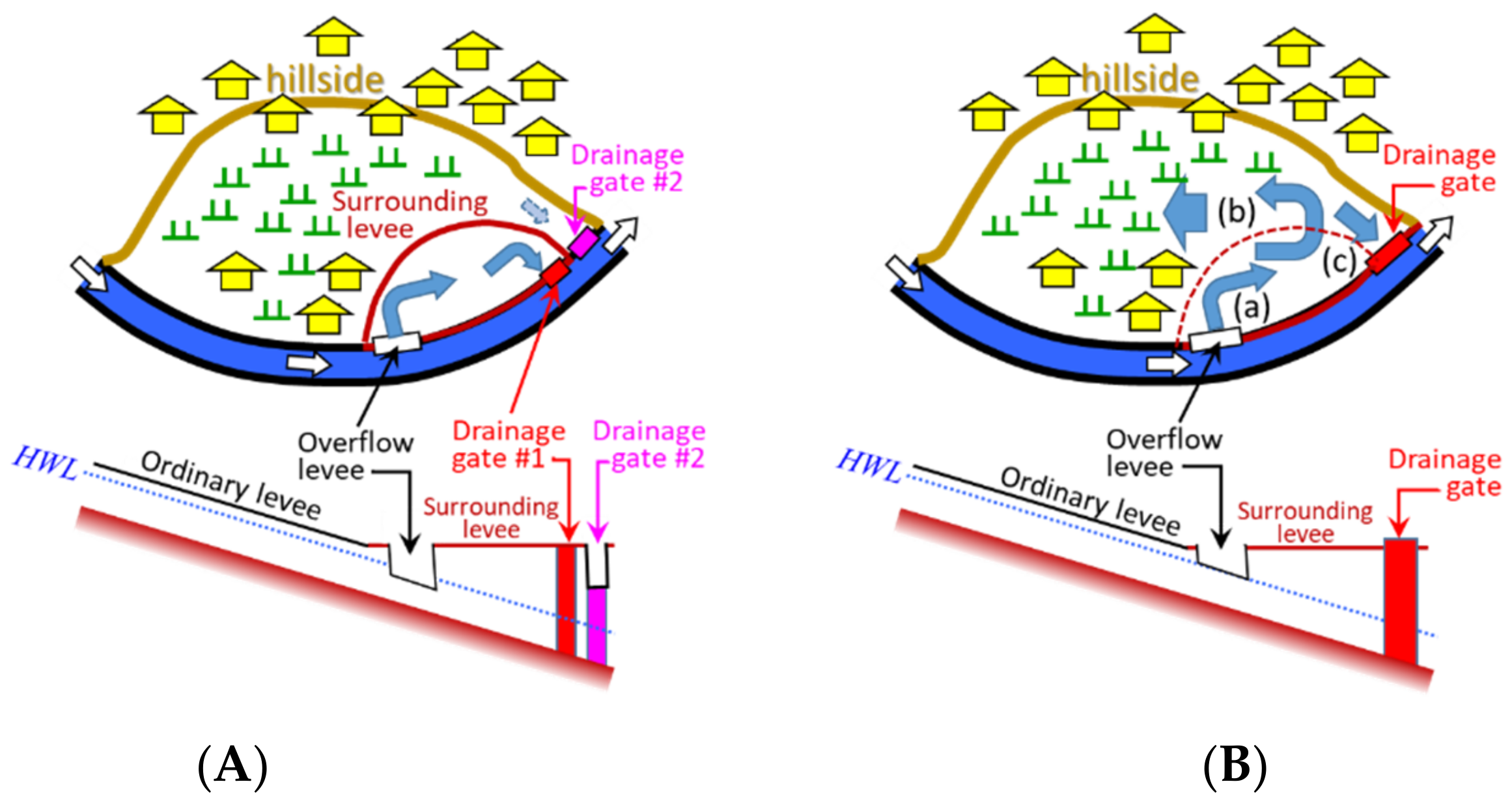
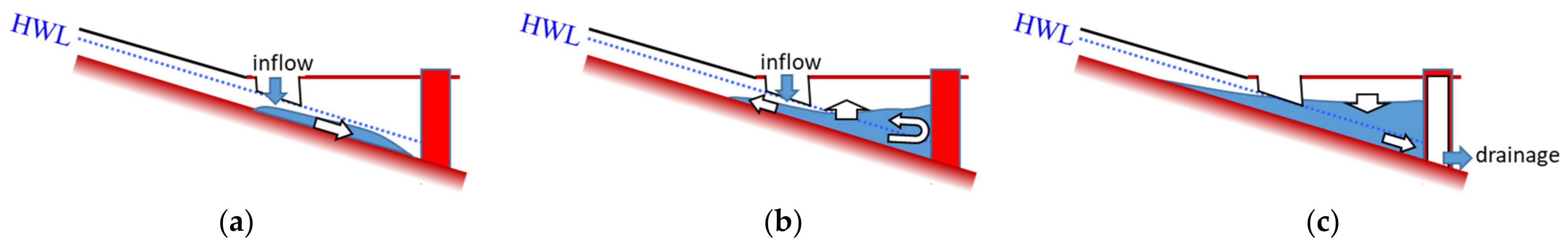
7.1. Remodeling Policy and Trial Design

The increased frequency of floods exceeding the discharge capacity of river channels due to global climate change is concerning, especially because it will take a long time and substantial funding to improve long river channels and build new flood control dams and detention basins. To alleviate this dilemma, we may consider two possible methods that are relatively simple, have low cost, and possibly could be implemented in a short time. One is to resize existing detention basins to increase flood control capabilities. The other is to accept some amount of flood damage by releasing the water volume that exceeds the capacity of the river channel into the floodplain as safely as possible. By combining these two ideas, a simple remodeling of the HDP is considered, and its effect is evaluated by a numerical experiment.

As explained in Section 2.2, in many small basins in the upper reaches of the Abukuma River, inundation was more frequent before the construction of levees than it is at present, and the basins functioned as natural water-detention basins. In fact, the houses are located on the hills around the basins and on the natural levees, even after the recent levee construction, and the parts of the floodplain with low elevation are used as paddy fields. Therefore, the settlements in these areas are considered to be able to accept some amount of flooding. Therefore, according to the concept explained in Section 2.3, we examined the improvement of the flood control capacity of the HDP by remodeling it into a borderless detention pond that gradually floods from the downstream side without hav-ing a surrounding embankment.

Figure 30 shows a schematic diagram of the facility improvement. Panel (a) shows the current HDP, the area of which is limited to about 1/5 of the total area of the basin by the surrounding levees. Houses and farmlands in this area were demolished, and the ground was excavated to increase the water storage capacity. However, as described in the previous section, the HDP quickly filled during the 2019 flood and did not contribute to reducing its peak.

Therefore, remodeling was considered as shown in panel (b). In the remodeled HDP, the surrounding levee on the land side of the HDP is removed and the top of the overflow weir is raised to the HWL. Villages and farmlands remain in the floodplain. Note that it is assumed that the levees with overtopping in 2019 are increased to a height sufficient to prevent recurrence. The thick arrows marked with (a), (b), or (c) indicate the expected flow pattern on the floodplain at each temporal stage, the side views of which is depicted in Figure 31 in the next page:

(a)

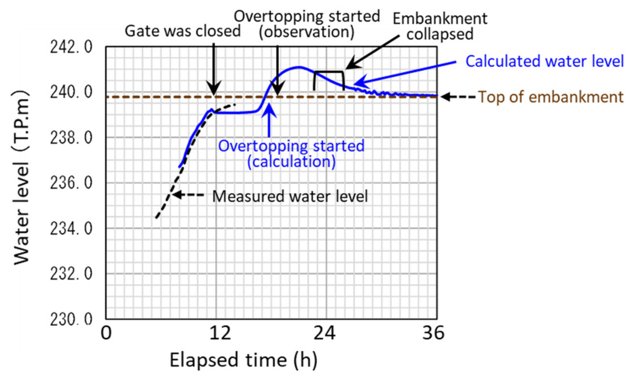
When the water level in the river channel exceeds HWL, some of the river water starts flowing onto the floodplain from the overflow weir and flows downstream along the floodplain slope.

(b)

After the flood flow reaches the downstream end of the basin, it forms a pond that gradually expands upstream due to the backwater.

(c)

When the river water level outside the drainage gate becomes lower than the land side water level, the gate is opened, and the stored water is discharged to the river.

As the result of surrounding levee removing, the relationship between the water level and the storage capacity of the HDP, as shown in Figure 15, is improved especially above the elevation of 239 T.P.m, which will become effective against excess runoff.

7.2. Numerical Simulation and Discussion

Figure 32 shows the flood hydrograph input into a numerical experiment to investigate the hydraulic effect of the modified facility. The maximum discharge and flood duration are the same as those of the 2019 flood (see Figure 25b), but the hydrograph was simplified to have a single peak. The downstream end condition of the calculation reflects the relationship between the flow rate and the water level at the Sukagawa Observatory shown in Figure 18b.

Figure 33 shows the temporal change in inundation depth (a–e) and the maximum depth distribution (f). The T in the figures corresponds to the elapse time shown in the hydrograph in Figure 32. The inundation started before T = 12:00, and just after the flood peak (T = 16:00), the HDP became almost full. After that, the inundation area expanded upstream until T = 20:00, and at T = 24:00, the river overflow had already ended, and the inundation area began shrinking. At T = 28:00, the inundation was almost over, except in the depression comprising the HDP.

Because most of the houses are located on hillsides and natural levees, the inundation depth was less than 1 m, as shown in Figure 33f. Therefore, it is thought that the flooding can be dealt with by relatively simple measures, such as raising the house base or surrounding the houses with a tall impermeable fence with a water stop gate that can be closed during flooding. Farmland, however, is flooded over a fairly large area. Therefore, the harvest may be lost once every few decades due to an excessive flood.

Figure 34 illustrates the flood control effects. Figure 34a compares the downstream end hydrographs obtained by the numerical simulations. The dotted curve is the hydrograph when without any flood control facility, and the difference from this line shows the flood control effect of existing HDP and remodeled HDP, cases (1) and (2), respectively. In case (1), the current HDP quickly filled before the flood peak and did not contribute to reducing the maximum flow rate. This is because, as mentioned in the previous section, the current HDP capacity is insufficient against the excess runoff. In case (2), on the other hand, a peak reduction of about 190 m³/s can be seen.

Figure 34b shows the rate of inflow from the overflow weir and the rate of drainage from the downstream gate in case (2). The drainage hydrograph has a time delay of about 8 h with respect to the inflow hydrograph, and the peak value is halved. Figure 34c shows the water levels on both sides of the drainage gate for case (2). Both water levels are about 2 m lower than the height of river embankment, and no overflow occurs.

Numerical simulation was performed also for a hydrograph having the same profile as that in Figure 32 but with a peak flow rate of 2400 m³/s, which corresponds to the maximum flood discharge written in the master plan. The results are shown in Figure 35 in the same way as in Figure 34. Figure 35a shows that the remodeled HDP reduces the flood peak by about 220 m³/s. In addition, Figure 35c shows that the water levels on both sides of the drainage gate are about 1 m lower than the height of the river embankment, and no overflow occurs. The results of this calculation suggest that the remodeled HDP will have some flood control effect, even for a runoff event larger than that in 2019.

8. Conclusions

The rapid increase of excess runoff due to global climate change will be unavoidable. However, at this time, flood data are limited due to the infrequency of excess runoff events in each basin and further, large floods often damage measuring equipment, accidentally creating periods without data. Therefore, it is not easy to establish new design standards for flood control facilities against excess runoff at this moment. In addition, considering budget constraints for flood control projects, it is desirable to remodel existing facilities by the simplest method possible.

Therefore, in the first part of this study, the flood control effect of the existing detention basin (HDP) during the excess runoff event that occurred on the Abukuma River in 2019 was analyzed by combining the fragmentary field observation data with numerical simulation. In the second part, in accordance with the MLIT’s new flood control policy to allow excess water to flow onto floodplains, a simple and low-cost remodeling method for the HDP was proposed and examined for its flood control effect.

In this remodeling plan, the surrounding levee on the upstream floodplain slope is removed, and the top of the overflow levee is raised to the HWL. As a result, the excess water volume exceeding the HDP’s capacity flows out to the upstream floodplain to expand the water surface area, and the flood control effect is greatly improved. Although the village in the upstream floodplain is flooded to some extent, it was confirmed that inundation damage could be sufficiently mitigated by simple improvements to house structures for waterproofing.

The numerical model used in this study is a simple one commonly used to estimate the inundation extent in river management works in Japan, which combines one-dimensional unsteady flow equations for a river channel and two-dimensional shallow water equations with regular rectangular grids for floodplains. Despite being a very simple model, the calculation results were in good overall agreement with observation data from the 2019 flood. This calculation is very fast, and the computation cost is low, so it is suitable for the rough design of flood control facilities.

For specific and detailed facility planning, numerical simulation using a more precise model will be required. For example, a numerical model using an unstructured triangular grid system [20] can express the effects of the existence of structures, such as houses and roads, in floodplains and the effects of trees in river channels on the flow field, but the calculation load is very high. Therefore, preliminary studies to readily compare alternatives possible under the given topographic and land use conditions are required. The approach using the simple model will be useful as demonstrated in this study.

References

- Japan Society of Civil Engineers Hydraulic Engineering Committee: Investigation Team Report on Western Japan Heavy Rain Disaster in July 2018. March 2019. (In Japanese)
- Japan Society of Civil Engineers Hydraulic Engineering Committee: Investigation Team Report on Typhoon No. 19 Heavy Rain Disaster in 2019. September 2020. (In Japanese)
- Japan Society of Civil Engineers Hydraulic Engineering Committee: Investigation Team Report on Kyushu Heavy Rain Dis-aster in July 2020. April 2021. (In Japanese)
- Japan Meteorological Agency: Long-Term Changes in Sea Surface Temperature (the Sea Near Japan), October 2021. Available online: https://www.data.jma.go.jp/gmd/kaiyou/data/shindan/a_1/japan_warm/japan_warm.html (accessed on 18 December 2021). (In Japanese)
- Ministry of Land, Infrastructure, Transport and Tourism (MLIT): River Basin Disaster Resilience and Sustainability by All, Japan’s New Policy on Water-Related Disaster Risk Reduction, November 2020. Available online: https://www.mlit.go.jp/river/kokusai/pdf/pdf21.pdf (accessed on 18 December 2021).
- MLIT: Rivers in Japan, P.40. Publication of the Flood-Prone Area Maps. Available online: https://www.mlit.go.jp/river/kokusai/pdf/pdf01.pdf (accessed on 18 December 2021).
- MLIT: Plans of River Basin Disaster Resilience and Sustainability by All for Each Nationally Managed Class-A River, March 2021. Available online: https://www.mlit.go.jp/river/kasen/ryuiki_pro/index.html (accessed on 15 April 2021). (In Japanese)
- MLIT. MLIT: Manual for Creating Flood Prone Area Maps, 4th ed.; MLIT: Tokyo, Japan, 2015. (In Japanese) [Google Scholar]
- Okuma, T. A study on the function and etymology of open levees. In Historical Studies in Civil Engineering, Japan; Japan Society of Civil Engineers: Tokyo, Japan, 1987; Volume 7, pp. 259–266. (In Japanese) [Google Scholar]
- Nemoto, Y.; Nakayama, D.; Matsuyama, H. Reevaluation of Shingen-tsutsumi base on inundation flow simulation with special focus on the flood control facilities along the Midai River. Geogr. Rev. Jpn. Ser. A 2011, 84, 553–571. (In Japanese) [Google Scholar]
- Ishikawa, T.; Akoh, R. Assessment of flood risk management in lowland Tokyo areas in the seventeenth century by numerical flow simulation. Environ. Fluid Mech. 2019, 19, 1295–1307. [Google Scholar] [CrossRef]
- Teramura, J.; Shimatani, Y. Advantages of the Open Levee (Kasumi-Tei), a Traditional Japanese River Technology on the Matsuura River, from an Ecosystem-Based Disaster Risk Reduction Perspective. Water 2021, 13, 480. [Google Scholar] [CrossRef]
- Ishikawa, T.; Senoo, H. Hydraulic Evaluation of the Levee System Evolution on the Kurobe Alluvial Fan in the 18th and 19th Centuries. Energies 2021, 14, 4406. [Google Scholar] [CrossRef]
- Ishida, T.; Maeda, Y. Investigation in the disaster management plan for future climate change. In KASEN; Japan River Association: Tokyo, Japan, 2020; Volume 890, pp. 15–19. (In Japanese) [Google Scholar]
- Landform Classification Map for Flood Control. Available online: https://www.gsi.go.jp/bousaichiri/bousaichiri41043.html (accessed on 30 April 2018). (In Japanese)
- Ito, Y.; Akoh, R.; Ishikawa, T.; Maeno, S. Numerical study on flood control function of levee openings located along valley bottom plain rivers in the past. J. Jpn. Soc. Civ. Eng. B1 Hydraul. Eng. 2018, 74, 1531–1536. (In Japanese) [Google Scholar]
- MLIT: Low Cost, Long Life, Localized 3L Water Level Gauge. Available online: https://www.mlit.go.jp/river/kokusai/pdf/pdf03.pdf (accessed on 15 October 2021).
- MLIT: Investigation Committee Report on Abukuma River Upstream Embankment, June 2020. (In Japanese)
- Honma, H. Coefficient of flow volume on low overflow weir. Proc. JSCE 1940, 26, 635–645. (In Japanese) [Google Scholar]
- Akoh, R.; Ishikawa, T.; Kojima, T.; Tomaru, M.; Maeno, S. High-resolution modeling of tsunami run-up flooding: A case study of flooding in Kamaishi city, Japan, induced by the 2011 Tohoku tsunami. Nat. Hazards Earth Syst. Sci. 2017, 17, 1871–1883. [Google Scholar] [CrossRef] [Green Version]