Age Estimation from fMRI Data Using Recurrent Neural Network

Abstract

Finding a biomarker that indicates the subject’s age is one of the most important topics in biology. Several recent studies tried to extract a biomarker from brain imaging data including fMRI data. However, most of them focused on MRI data, which do not provide dynamics and lack attempts to apply recently proposed deep learning models. We propose a deep neural network model that estimates the age of a subject from fMRI images using a recurrent neural network (RNN), more precisely, a gated recurrent unit (GRU). However, applying neural networks is not trivial due to the high dimensional nature of fMRI data. In this work, we propose a novel preprocessing technique using the Automated Anatomical Labeling (AAL) atlas, which significantly reduces the input dimension. The proposed dimension reduction technique allows us to train our model with 640 training and validation samples from different projects under mean squared error (MSE). Finally, we obtain the correlation value of 0.905 between the predicted age and the actual age on 155 test samples. The proposed model estimates the age within the range of $\pm 12$ on most of the test samples. Our model is written in Python and is freely available for download.

1. Introduction

Understanding human aging and anti-aging are important topics in biology [1,2,3,4,5]. One way of understanding aging is finding a biomarker that indicates the physical age of subjects. Many studies have been conducted to try to estimate age using biological data [6,7,8,9,10,11]. Among various sources of biological data, the brain is one of the most complex and critical parts of human beings. Since the structure of the brain also varies with age [12,13,14,15,16], it is natural to extract a biomarker from brain-related data [17,18]. Recently, the research on the brain has mainly focused on neuroimaging technology [19,20,21,22,23,24,25,26]. In particular, functional magnetic resonance imaging (fMRI) is widely used [27,28,29] because it provides a time series of 3D images in a non-invasive manner [30,31].

The relationship between the brain and age through neuroimages has been explored [32,33,34,35,36]. Franke et al. [37] showed the relationship between the human brain and age through MRI data, which is a static image of the brain. The authors used principal component analysis to reduce the size of the MRI data and performed regression analysis by training the relevance vector machine (RVM) to estimate the age of the subject. Recently, deep learning networks have been used to analyze MRI images. Huang et al. used the VGGNet [38] to extract features from MRI images [39]. Qi et al. proposed a 3D convolutional neural network (CNN) for the 3D level of MRI images [40]. Jiang et al. conducted a comparative study of T1-weighted brain images at different parts (gray matter, white matter, and cerebrospinal fluid) through a DenseNet [41] based on transfer learning [42]. However, the authors used a still image of the brain at rest and did not consider the brain function network dynamics over time.

Brain function network dynamics suggest that human brain activity is not only an activity of a single functional brain area but also a time-varying interaction between multiple areas [43,44]. Furthermore, fMRI is more sensitive to detecting aging-related neurodegenerative diseases [45]. Thus, an age estimation based on fMRI has an advantage over structural MRI. Yao et al. showed the relationship between the entropy of the brain and age [46] including time-varying dynamics. The authors first divided the fMRI image into 90 regions using the Automated Anatomical Labeling atlas (AAL) [47], then transformed the fMRI image to time series data. Finally, they extracted correlation coefficients among all the pairs of the time series and computed the entropy of the empirical distribution of coefficients. However, the correlation between the entropy and the actual age is not strong, and it is hard to interpret the meaning of the entropy of coefficients.

Another area related to time series data is natural language processing (NLP). Recurrent neural networks (RNN) [48], long short-term memory (LSTM) [49], and gated recurrent units (GRU) [50] dominated the field due to their structure being similar to time series. Later, Transformer [51], based on a simple and clear attention structure [52,53], was proposed, which showed more concise and efficient performance than traditional deep networks. Transformer achieves better results due to its ability to capture long-term dependencies.

In this paper, we propose a deep neural network (DNN) model to estimate the age from fMRI. Since fMRI data can be viewed as a time series of 3D images, it is natural to use network models from NLP, such as recurrent neural networks (RNN) or Transformer. The proposed model is based on GRU since fMRI data have weaker long-term dependencies.

We would like to emphasize that applying an existing DNN model is not trivial, mainly due to the data shortage issue. The cost of collecting fMRI data is high, and it is hard to obtain a sufficient amount of data to train the DNN model. Moreover, the dimension of fMRI data is huge (e.g., $64\times 64\times 34\times 100$) compared to the number of trainable data. To overcome the data shortage, we propose a new dimension reduction technique for fMRI data. More precisely, we use fMRI data from 795 publicly available samples. We first apply the clustering algorithm to the data to reduce the dimension. This provides time series data that are a 94 dimension vector at each repetition time point. Then, we train DNN models that estimate the age, where the input is preprocessed fMRI data. We compare the proposed model with other DNN models including vanilla RNN, Transformer, and multilayer perceptron (MLP). The correlation coefficient between the estimated age and the actual age is $r=0.905$, which outperforms the other DNN models.

The paper is organized as follows. In Section 2, we provide detailed information about fMRI samples and introduce the preprocessing step that reduces the input dimension. The proposed recurrent neural network-based model is described in Section 3. We provide an experimental setup and results in Section 4. In Section 5, we investigate the overall contribution of components to the proposed model, and we conclude the paper in Section 6.

2. Methods

2.1. Data Acquisition

We collect a total of 1450 human brain fMRI samples from 26 publicly available projects, where informed consent was obtained from all subjects. Defective samples are removed including samples with no age information and samples with incomplete data. Finally, we use a total of 795 samples of fMRI data consisting of 437 women and 358 men. The range of ages is from 10 to 80.

Table 1. Detailed information of data collection. (M: Male; F: Female; $N_{TR}$: the number of repetition time points).

Project	Subjects	Age	M	F	${\mathit{N}}_{\mathbf{TR}}$
AnnArbor_a	18	13–40	17	1	283
Baltimore	12	30–40	6	6	111
Bangor	3	19	3	0	253
Beijing_Zang	39	18–24	21	18	213
Berlin_Margulies	14	23–44	7	7	183
Cambridge_Buckner	81	18-30	30	51	107
Dallas	14	20–71	8	6	103
ICBM	35	19–79	15	20	116
Leiden_2180	3	20–27	3	0	203
Leiden_2200	4	18–25	4	0	203
Leipzig	15	22–42	7	8	183
Milwaukee_b	46	44–65	15	31	163
Newark	7	21–39	4	3	123
NewHaven_a	2	18–38	2	0	237
NewHaven_b	6	18–42	4	2	169
NewYork_a	37	10–49	20	17	180
NewYork_a_ADHD	16	24–50	15	1	180
NewYork_b	11	18–46	7	4	163
Orangeburg	14	31–55	11	3	153
Oulu	17	21–22	4	13	233
Oxford	8	30–35	6	2	163
PaloAlto	12	26–46	1	11	223
Pittsburgh	1	27	1	0	263
Queensland	6	21–34	4	2	178
SaintLouis	5	21–28	3	2	115
SALD	369	19–80	140	229	230

provides the statistics of data.

SALD project has 369 samples from the Southwest University Adult Lifespan Dataset (SALD) [54]. The sample includes 229 women and 140 men, who are students and residents from the Southwest University of China. All other projects are from the 1000 Functional Connectomes Project (http://fcon1000.projects.nitrc.org, accessed on 20 November 2021), with a total of 426 brain samples, including 208 women and 218 men.

Since the data are obtained from various projects, some inconsistencies are hard to be normalized. Specifically, the repetition times (TR) vary from 1 to 3 s. Among 795 samples, 629 samples have a TR of 2 s, and the majority of the remaining samples have TRs close to 2 s. Since most of them have similar TRs, we ignore the impact of TR differences in this work. For the positional variation, we normalize the data, which is described in the following section.

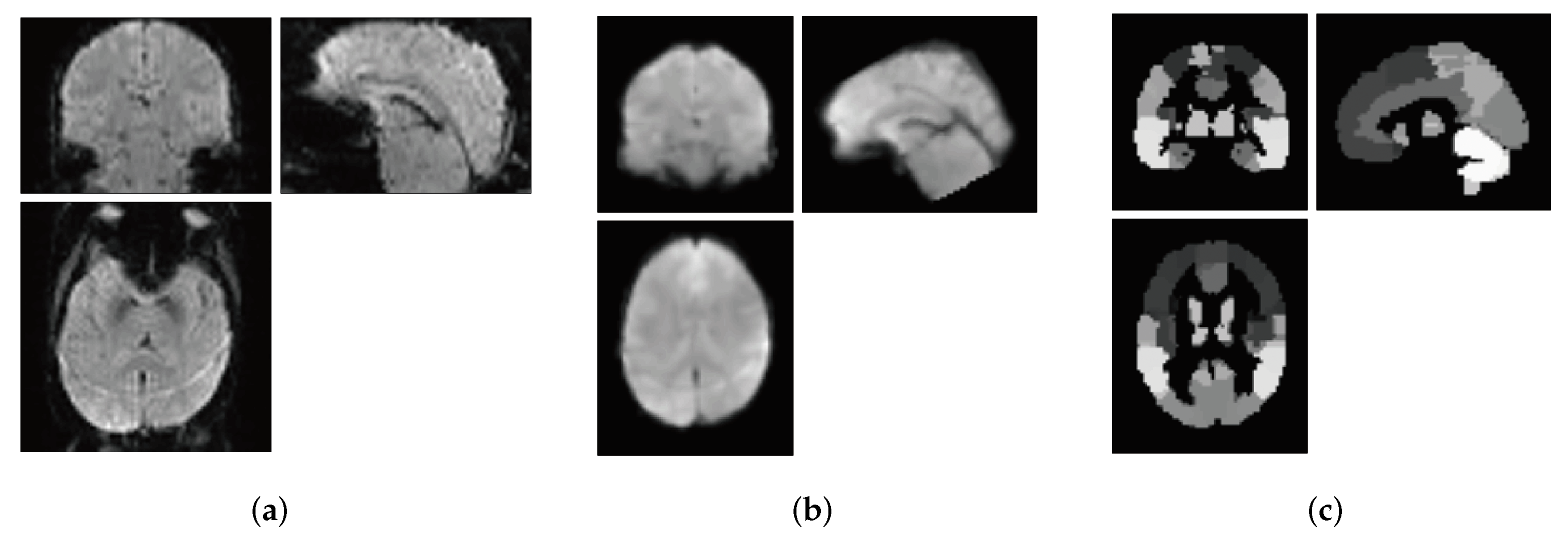
2.2. Data Preprocessing

The fMRI scanner often performs environmental adaptation at the beginning of the scan. It is also unstable during the adaptation, which may provide inconsistent data. To avoid this issue, we discard the earliest part of fMRI data (the first 10 repetition time points).

Since we collect the data from various projects, each project may have its own setups or imaging parameters. In other words, each project may have its own bias, and therefore we need to remove the bias from each project. Moreover, each subject may have different sizes of brains, and the brain positions might vary while scanning. These variations in the sample can impact our model since the size of the dataset is not large enough. To resolve the issue, we apply a normalization technique for the individual data.

First, we use the FMRIB software library (FSL) to preprocess fMRI data. FSL is a widely used tool for brain imaging data [55,56]. More precisely, we employ the FEAT toolbox in the FSL software library to normalize the fMRI data. To remove the bias of the project, we extract imaging parameters from each project and center the images of the project with corresponding parameters.

The second part of the preprocessing is the registration of the normalized image. The registration step clusters the image to several regions accordingly and provides a “mask” that indicates the coverage of regions. Among various registration methods, we use AAL2 from the Montreal Institute of Neurology (MNI) brain space Automated Anatomical Labeling atlas (AAL) [57]. FMRIB Linear Image Registration Tool (FLIRT) is used for registration, which is an automation tool for brain image registration in the FSL software library. This registration step divides the brain into 94 regions of interest (ROI). Note that the above steps do not reduce the dimension of data and the original data can be recovered by reversing the process. An example of normalization and registration of fMRI images is shown in Figure 1.

After the registration step, we average the voxel values of each region to reduce the dimension of data. Thus, after the preprocessing, we obtain a time series data X of length t. More precisely, let C be the fMRI sample and $f_{pre}$ be the preprocessing procedure including normalization, registration, and averaging. Then, we obtain the time series data $X=(x_1,x_2,\cdots ,x_t)=f_{pre}\left(C\right)\in {\mathbb{R}}^{94\times t}$, where the preprocessed brain image at the i-th repetition time point $X_i\in {\mathbb{R}}^{94}$ is a 94-dimensional vector. Note that fMRI data from different projects may have different repetition time points. The whole preprocessing steps are depicted in Figure 2.

3. Age Estimation

3.1. Preliminaries

Since the preprocessed data is a time series that reflects brain function network dynamics, it is natural to consider the neural network (NN) models designed for sequence data, such as recurrent neural networks (RNN) and Transformer. RNN recursively summarizes the sequential data and analyzes its dynamic behavior [48]. However, RNN has vanishing and exploding gradient issues. Long short-term memory (LSTM) introduced gates to solve this issue [49,58]. The gated recurrent unit (GRU) is a variant of the LSTM network, which has a simpler and more effective structure [50,59]. We propose a GRU-based model for age estimation. We also provide several other DNN models for baseline. In Section 4, we provide a comparison between the proposed model and the other baseline models.

3.2. Proposed Model

The proposed GRU-based model takes an input X, where the last GRU is followed by fully connected (FC) layers, including a batch normalization (BN) layer and ReLU activation. We describe the structure of the proposed model in Figure 3a. The model hyperparameters, including the number of layers and hidden dimensions, are optimized as described in Section 4.

Other Baseline Models

Another estimator we considered is a Transformer, which shows extraordinary performances in NLP such as translation. The Transformer generally includes two parts. The ”encoder” takes an input sequence then maps to a vector where the “decoder” outputs a sequence based on the encoded vector. Since we want to estimate age (real number), we are only interested in the Transformer encoder. Similar to Transformer-based models in NLP, we first map the preprocessed data X to a vector using positional encoding. Then, we apply multiple Transformer encoder layers that consist of self-attention and feed-forward layers. The final fully connected layers estimate the age. The structure of Transformer-based model is described in Figure 3a.

We also considered the other RNN-based models, including vanilla RNN and LSTM, where vanilla RNN and LSTM also have similar structures to the GRU-based model.

Finally, we constructed a multilayer perceptron (MLP) that consists of FC layers only. We treat the preprocessed fMRI data as data with two dimensions: time series and brain regions. We constructed a multi-layer model learning data with the same structure. Each layer contains an FC layer, a batch normalization (BN) layer, a ReLU activation, and a dropout [60].

4. Experiments

4.1. Model Parameters

Hyperparameters of models are optimized via cross-validation as described in Section 4.2. The proposed GRU-based model has three internal layers where each recurrent unit has 300 hidden states, and the width of the final FC layer is 300. The Transformer network consists of three Transformer encoder layers, where each layer consists of two sub-layers. The first is the multi-head self-attention mechanism: we set the number of heads to 2. The second is a position-wise feed-forward layer that sets its network dimension to 8 times the input dimension. We optimize other RNN-based models (vanilla RNN and LSTM) and achieve the same hyperparameters as the GRU-based model. The MLP network consists of three FC layers. Standard dropout probability $p=0.5$ is used in RNN- and MLP-based models. In the Transformer model, the dropout probability of $p=0.1$ is used in the positional encoding and the encoder layer.

4.2. Training

The data are divided into three independent sets: training, validation, and test sets. We first divide all the data into two parts, with a ratio of 8 to 2 as shown in

Table 2. Data volume distribution of training, validation, and test datasets.

Training/Validation	Test
640	155

. In all, 20% of the total data, namely 155 samples, are assigned for the test. The remaining 80% of the total data, namely 640 samples, are used for training and validation.

We use k-fold cross-validation with $k=10$ due to an insufficient amount of data. The data except for the test set (total 640 data points) are divided into 10 subsets, one subset is used as the validation dataset and the other 9 subsets are used as the training dataset. This procedure is repeated 10 times, then the average performance is computed. We choose the model hyperparameters that provide the best average performance.

For model training, we use the Adam optimizer with learning rate attenuation. The initial learning rate value is set to 0.001 for the GRU model and 0.0001 for the Transformer model. The learning rate is attenuated by 0.99 every 100 steps. In our experiment, the training batch size is set to 144 where the number of epochs is 10,000. The mean squared error (MSE) is employed to compute the loss while training

$$MSE=\frac{1}{n}\sum _{i=1}^n{(f_{NN}\left(X^{\left(i\right)}\right)-y^{\left(i\right)})}^2$$

where $(X^{\left(1\right)},y^{\left(1\right)}),\cdots ,(X^{\left(n\right)},y^{\left(n\right)})$ denotes the preprocessed data sample and label pair, and $f_{NN}(·)$ denotes a proposed neural network. Thus, the training is to minimize MSE.

4.3. Implementations

Our neural network model and data preprocessing procedures are implemented in Python, which is freely available for download at https://github.com/gyfbianhuanyun/brain-data-with-age (accessed on 20 November 2021). The machine used to perform the experiments has the following specifications: 8 GB RAM, Intel(R) Core(TM) i5-8400 @2.80GHz CPU processor, and Nvidia Geforce GTX 1050 graphics card.

4.4. Results

Table 3. Correlation between the estimated age and the actual age on the test dataset.

Model Name	Regions	Correlation	MSE	MAE	ICC
MLP	All	0.780	140.09	8.645	0.754
RNN	All	0.797	110.28	7.935	0.774
LSTM	All	0.858	116.48	8.627	0.812
GRU	All	0.905	70.76	6.507	0.883
GRU	Right	0.769	132.49	8.630	0.754
GRU	Left	0.835	110.69	8.850	0.807
Transformer	All	0.883	74.44	6.566	0.884

shows the performance of the proposed model and other baseline models on the test dataset (155 data points). It provides the correlation between estimated age and the actual age. In addition to MSE, we compute the mean absolute error (MAE) to measure the accuracy of age estimation

$$MAE=\frac{1}{n}\sum _{i=1}^n|f_{NN}(X^{\left(i\right)}-y^{\left(i\right)}|$$

We also provide the intraclass correlation coefficient (ICC) to evaluate the model’s performance. The ICC evaluates the consistency of the same number of measurement results measured by multiple observers. Here, we take the actual age and the predicted age as two measurement results and judge the prediction model’s performance by the degree of consistency.

The GRU model shows the best performance while the Transformer model has comparable results. Figure 4a shows the performance of the GRU model where the x-axis shows the age of the subject and the y-axis represents the estimated age by the proposed model. The gender of the subjects are indicated where blue dots represent male subjects, and red triangles represent female subjects. It can be seen that more than 80% of the estimations are within the $\pm 12$ range of the actual age. The correlation coefficient between the estimation and the actual age is $r=0.905$.

The training results using the Transformer model are shown in Figure 4b. These results will be discussed in Section 4.5. Since most previous works [37,39,40,42] focus on structural MRI input and codes are not available online, we compare our results with Yao et al. [46], which computes a correlation between entropy and actual age based on fMRI data samples. Figure 4c shows the relation between entropy and age. The correlation coefficient between the entropy and the age is $r=0.292$, which is weaker than the proposed estimation model.

In addition, we provide Bland–Altman plots to visualize the results. The Bland–Altman plot shows the consistency between two different measurements. Here, we use the actual age of the test data sets as a known measurement and the predicted age as another measurement value. Figure 4d,e show Bland–Altman plots of the GRU model and Transformer model. What needs attention here is the processing of the entropy results. Since the entropy value is not an age estimation, we first find a linear regression model that estimates an age from the entropy value. Figure 4f shows a Bland–Altman plot of estimated age from entropy and the actual age.

4.5. Discussion

4.5.1. Age Bias

As we can see in Figure 4a, our model tends to underestimate the age of subjects. This is mainly due to a bias of our training dataset where we have more young subjects in the training set, as we showed in Table 1. More precisely, the number of subjects younger than 30 is 256, which is 32.20% of the dataset, while the number of subjects older than 60 is 144, which is 18.11% of the dataset.

4.5.2. Gender Difference

Figure 4a shows the gender difference of our model. For female subjects, the estimation is more accurate for samples of those aged around 20, but the estimation becomes less accurate when the age of a sample is more than 60. On the other hand, for male subjects, the estimation loss is consistent throughout the ages. Note that Yao et al. [46] also reported the gender difference. The authors mentioned that the functional entropy increases with age where the mean entropy of female subjects increases slower than male subjects.

5. Ablation Study

We also trained the GRU-based model with variations.

5.1. Effect of Brain Regions

In order to analyze the influence of different brain regions on the results, we extracted the parts with left or right hemispheres in the brain region named in the AAL2 atlas and conducted the training. Table 3 shows the training results. We found that under the same conditions, it is beneficial to fully utilize all the available brain regions to estimate the age of subjects. Interestingly, we observed that the data from the left hemisphere have a higher correlation with age.

5.2. Effect of Dropout

As we mentioned in the above section, we employ the dropout technique to prevent overfitting. Figure 5a,d show the estimation result of the exact same model without dropout. It can be seen that some estimations deviate from the actual ages, where the proposed method with dropout shows a robust estimation. The correlation coefficient without dropout is $r=0.849$, which is smaller than the correlation coefficient $r=0.905$ of the proposed model in the presence of dropout. This clearly shows that the dropout suppresses the generalization error, especially in our case where the size of the dataset is small.

5.3. Choice of Loss Function

Since the ${\ell }_1$ loss function and the MSE (${\ell }_2$) loss function are relatively common loss calculation methods, in this section, we investigate how the choice of loss function affects the result. Figure 5b,e show the estimation result when the ${\ell }_1$ loss function is employed. The estimation with ${\ell }_1$ loss is less accurate than the model with the MSE loss function. This is because the MSE loss penalizes the large errors more while the ${\ell }_1$ loss function computes the absolute deviation. In particular, we can see some outliers when we train the model with the ${\ell }_1$ loss function. Note that the correlation coefficient of the model is $r=0.749$.

5.4. Effect of Scan Time

To see the effect of time dynamics on brain imaging data, we train the model with samples that are fixed length time series. Figure 5c,f show the estimated result when the model uses the first 100 repetition time points only. In this case, the model correlation coefficient is $r=0.889$, which is lower than the result of using all times data. This shows that the brain function network dynamics are indeed helpful in age estimation.

6. Conclusions

To estimate the age from fMRI images, we proposed the deep learning model based on GRU and Transformer. The preprocessing technique is also provided to reduce the data dimension. Since we have only 795 pieces of data, we use cross-validation to determine hyperparameters during training. Despite the lack of data, our model provides a reasonable estimation of age compared to the previous entropy-based method. Throughout the research, we found a relationship between brain activity and age, which can be extended to other brain disease research.

Limitations: Since the proposed GRU-based model takes a preprocessed input, the region extraction method is crucial. The proposed framework is based on the AAL atlas, an anatomical (structural) parcellation. We would like to mention that other representations such as functionally-defined brain regions of interest [61,62,63] might be more sensitive to analyzing fMRI. However, our framework is universal in the sense that we can apply the same normalization technique and GRU-based model even with functionally-defined regions of interest. Another limitation is the diversity of data samples obtained from different projects. Although we normalized samples during preprocessing, this may cause inter-project errors. In future work, we plan to collect samples from controlled experiments.

References

1. Havighurst, R.J. Successful aging. Process. Aging Soc. Psychol. Perspect. 1963, 1, 299–320. [Google Scholar]
2. Hannum, G.; Guinney, J.; Zhao, L.; Zhang, L.; Hughes, G.; Sadda, S.; Klotzle, B.; Bibikova, M.; Fan, J.B.; Gao, Y.; et al. Genome-wide methylation profiles reveal quantitative views of human aging rates. Mol. Cell 2013, 49, 359–367. [Google Scholar] [CrossRef] [Green Version]
3. Balaban, R.S.; Nemoto, S.; Finkel, T. Mitochondria, oxidants, and aging. Cell 2005, 120, 483–495. [Google Scholar] [CrossRef] [Green Version]
4. Rowe, J.W.; Kahn, R.L. Successful aging. Gerontologist 1997, 37, 433–440. [Google Scholar] [CrossRef] [PubMed]
5. Blagosklonny, M.V. Aging-suppressants: Cellular senescence (hyperactivation) and its pharmacologic deceleration. Cell Cycle 2009, 8, 1883–1887. [Google Scholar] [CrossRef] [Green Version]
6. Ellingham, S.; Adserias-Garriga, J. Chapter 1—Complexities and considerations of human age estimation. In Age Estimation, 1st ed.; Adserias-Garriga, J., Ed.; Academic Press: Cambridge, MA, USA, 2019; pp. 1–15. [Google Scholar] [CrossRef]
7. Seok, J.; Kasa-Vubu, J.; DiPietro, M.; Girard, A. Expert system for automated bone age determination. Expert Syst. Appl. 2016, 50, 75–88. [Google Scholar] [CrossRef]
8. Zaghbani, S.; Boujneh, N.; Bouhlel, M.S. Age estimation using deep learning. Comput. Electr. Eng. 2018, 68, 337–347. [Google Scholar] [CrossRef]
9. Dimri, G.P.; Lee, X.; Basile, G.; Acosta, M.; Scott, G.; Roskelley, C.; Medrano, E.E.; Linskens, M.; Rubelj, I.; Pereira-Smith, O. A biomarker that identifies senescent human cells in culture and in aging skin in vivo. Proc. Natl. Acad. Sci. USA 1995, 92, 9363–9367. [Google Scholar] [CrossRef] [Green Version]
10. Krishnamurthy, J.; Torrice, C.; Ramsey, M.R.; Kovalev, G.I.; Al-Regaiey, K.; Su, L.; Sharpless, N.E. Ink4a/Arf expression is a biomarker of aging. J. Clin. Investig. 2004, 114, 1299–1307. [Google Scholar] [CrossRef] [PubMed]
11. Blackburn, E.H.; Greider, C.W.; Szostak, J.W. Telomeres and telomerase: The path from maize, Tetrahymena and yeast to human cancer and aging. Nat. Med. 2006, 12, 1133. [Google Scholar] [CrossRef] [PubMed]
12. Raz, N.; Gunning, F.M.; Head, D.; Dupuis, J.H.; McQuain, J.; Briggs, S.D.; Loken, W.J.; Thornton, A.E.; Acker, J.D. Selective aging of the human cerebral cortex observed in vivo: Differential vulnerability of the prefrontal gray matter. Cereb. Cortex 1997, 7, 268–282. [Google Scholar] [CrossRef] [Green Version]
13. Dixon, R.; Backman, L.; Nilsson, L. Part 3, Chapter 6—The aging brain: Structural changes and their implications for cognitive aging. In New Frontiers in Cognitive Aging, 1st ed.; Raz, N., Ed.; Oxford University Press: Oxford, UK, 2004; pp. 115–133. [Google Scholar] [CrossRef]
14. Salat, D.H.; Buckner, R.L.; Snyder, A.Z.; Greve, D.N.; Desikan, R.S.; Busa, E.; Morris, J.C.; Dale, A.M.; Fischl, B. Thinning of the cerebral cortex in aging. Cereb. Cortex 2004, 14, 721–730. [Google Scholar] [CrossRef] [Green Version]
15. Park, D.C.; Reuter-Lorenz, P. The adaptive brain: Aging and neurocognitive scaffolding. Annu. Rev. Psychol. 2009, 60, 173–196. [Google Scholar] [CrossRef] [PubMed] [Green Version]
16. Fjell, A.M.; Walhovd, K.B. Structural brain changes in aging: Courses, causes and cognitive consequences. Rev. Neurosci. 2010, 21, 187–222. [Google Scholar] [CrossRef] [PubMed]
17. Montagne, A.; Barnes, S.R.; Sweeney, M.D.; Halliday, M.R.; Sagare, A.P.; Zhao, Z.; Toga, A.W.; Jacobs, R.E.; Liu, C.Y.; Amezcua, L.; et al. Blood-brain barrier breakdown in the aging human hippocampus. Neuron 2015, 85, 296–302. [Google Scholar] [CrossRef] [Green Version]
18. Bae, S.H.; Kim, H.W.; Shin, S.; Kim, J.; Jeong, Y.H.; Moon, J. Decipher reliable biomarkers of brain aging by integrating literature-based evidence with interactome data. Exp. Mol. Med. 2018, 50, 28. [Google Scholar] [CrossRef] [PubMed] [Green Version]
19. Koenigsberg, R.A.; Bianco, B.A.; Faro, S.H.; Stickles, S.; Hershey, B.L.; Siegal, T.L.; Mohamed, F.B.; Dastur, C.K.; Tsai, F.Y. Chapter 23—Neuroimaging. In Textbook of Clinical Neurology, 3rd ed.; Goetz, C.G., Ed.; W.B. Saunders: Philadelphia, PA, USA, 2007; pp. 437–476. [Google Scholar] [CrossRef]
20. Goldstein, J.M.; Seidman, L.J.; Horton, N.J.; Makris, N.; Kennedy, D.N.; Caviness, V.S., Jr.; Faraone, S.V.; Tsuang, M.T. Normal sexual dimorphism of the adult human brain assessed by in vivo magnetic resonance imaging. Cereb. Cortex 2001, 11, 490–497. [Google Scholar] [CrossRef] [PubMed]
21. Giedd, J.N.; Snell, J.W.; Lange, N.; Rajapakse, J.C.; Casey, B.; Kozuch, P.L.; Vaituzis, A.C.; Vauss, Y.C.; Hamburger, S.D.; Kaysen, D.; et al. Quantitative magnetic resonance imaging of human brain development: Ages 4–18. Cereb. Cortex 1996, 6, 551–559. [Google Scholar] [CrossRef] [PubMed] [Green Version]
22. Pfefferbaum, A.; Mathalon, D.H.; Sullivan, E.V.; Rawles, J.M.; Zipursky, R.B.; Lim, K.O. A quantitative magnetic resonance imaging study of changes in brain morphology from infancy to late adulthood. Arch. Neurol. 1994, 51, 874–887. [Google Scholar] [CrossRef]
23. Giedd, J.N.; Blumenthal, J.; Jeffries, N.O.; Castellanos, F.X.; Liu, H.; Zijdenbos, A.; Paus, T.; Evans, A.C.; Rapoport, J.L. Brain development during childhood and adolescence: A longitudinal MRI study. Nat. Neurosci. 1999, 2, 861. [Google Scholar] [CrossRef]
24. Sowell, E.R.; Peterson, B.S.; Thompson, P.M.; Welcome, S.E.; Henkenius, A.L.; Toga, A.W. Mapping cortical change across the human life span. Nat. Neurosci. 2003, 6, 309. [Google Scholar] [CrossRef]
25. Giedd, J.N. The teen brain: Insights from neuroimaging. J. Adolesc. Health 2008, 42, 335–343. [Google Scholar] [CrossRef] [PubMed]
26. Cox, D.D.; Savoy, R.L. Functional magnetic resonance imaging (fMRI)”brain reading”: Detecting and classifying distributed patterns of fMRI activity in human visual cortex. Neuroimage 2003, 19, 261–270. [Google Scholar] [CrossRef]
27. Logothetis, N.K.; Pauls, J.; Augath, M.; Trinath, T.; Oeltermann, A. Neurophysiological investigation of the basis of the fMRI signal. Nature 2001, 412, 150. [Google Scholar] [CrossRef]
28. Madden, D.J.; Spaniol, J.; Whiting, W.L.; Bucur, B.; Provenzale, J.M.; Cabeza, R.; White, L.E.; Huettel, S.A. Adult age differences in the functional neuroanatomy of visual attention: A combined fMRI and DTI study. Neurobiol. Aging 2007, 28, 459–476. [Google Scholar] [CrossRef] [Green Version]
29. Dennis, E.L.; Thompson, P.M. Functional brain connectivity using fMRI in aging and Alzheimer’s disease. Neuropsychol. Rev. 2014, 24, 49–62. [Google Scholar] [CrossRef]
30. Brown, R.W.; Cheng, Y.C.N.; Haacke, E.M.; Thompson, M.R.; Venkatesan, R. Magnetic Resonance Imaging: Physical Principles and Sequence Design; John Wiley & Sons: Hoboken, NJ, USA, 2014. [Google Scholar]
31. Huettel, S.A.; Song, A.W.; McCarthy, G. Functional Magnetic Resonance Imaging; Sinauer Associates: Sunderland, MA, USA, 2004; Volume 1. [Google Scholar]
32. Giorgio, A.; Santelli, L.; Tomassini, V.; Bosnell, R.; Smith, S.; De Stefano, N.; Johansen-Berg, H. Age-related changes in grey and white matter structure throughout adulthood. Neuroimage 2010, 51, 943–951. [Google Scholar] [CrossRef] [PubMed] [Green Version]
33. Fonov, V.; Evans, A.C.; Botteron, K.; Almli, C.R.; McKinstry, R.C.; Collins, D.L.; The Brain Development Cooperative Group. Unbiased average age-appropriate atlases for pediatric studies. Neuroimage 2011, 54, 313–327. [Google Scholar] [CrossRef] [Green Version]
34. Meunier, D.; Achard, S.; Morcom, A.; Bullmore, E. Age-related changes in modular organization of human brain functional networks. Neuroimage 2009, 44, 715–723. [Google Scholar] [CrossRef]
35. Ota, M.; Obata, T.; Akine, Y.; Ito, H.; Ikehira, H.; Asada, T.; Suhara, T. Age-related degeneration of corpus callosum measured with diffusion tensor imaging. Neuroimage 2006, 31, 1445–1452. [Google Scholar] [CrossRef] [PubMed]
36. Richards, J.E.; Sanchez, C.; Phillips-Meek, M.; Xie, W. A database of age-appropriate average MRI templates. Neuroimage 2016, 124, 1254–1259. [Google Scholar] [CrossRef] [PubMed] [Green Version]
37. Franke, K.; Ziegler, G.; Klöppel, S.; Gaser, C. The Alzheimer’s Disease Neuroimaging Initiative. Estimating the age of healthy subjects from T1-weighted MRI scans using kernel methods: Exploring the influence of various parameters. Neuroimage 2010, 50, 883–892. [Google Scholar] [CrossRef] [PubMed]
38. Simonyan, K.; Zisserman, A. Very Deep Convolutional Networks for Large-Scale Image Recognition. In Proceedings of the 3rd International Conference on Learning Representations (ICLR 2015), San Diego, CA, USA, 7–9 May 2015. [Google Scholar]
39. Huang, T.W.; Chen, H.T.; Fujimoto, R.; Ito, K.; Wu, K.; Sato, K.; Taki, Y.; Fukuda, H.; Aoki, T. Age estimation from brain MRI images using deep learning. In Proceedings of the 2017 IEEE 14th International Symposium on Biomedical Imaging (ISBI 2017), Melbourne, Australia, 18–21 April 2017; pp. 849–852. [Google Scholar]
40. Qi, Q.; Du, B.; Zhuang, M.; Huang, Y.; Ding, X. Age estimation from MR images via 3D convolutional neural network and densely connect. In Proceedings of the International Conference on Neural Information Processing (ICONIP 2018), Bangkok, Thailand, 23–27 November 2020; Springer: Cham, Switzerland, 2018; pp. 410–419. [Google Scholar]
41. Huang, G.; Liu, Z.; Van Der Maaten, L.; Weinberger, K.Q. Densely connected convolutional networks. In Proceedings of the IEEE Conference on Computer Vision and Pattern Recognition (CVPR 2017), Honolulu, HI, USA, 21–26 July 2017; pp. 4700–4708. [Google Scholar]
42. Jiang, H.; Guo, J.; Du, H.; Xu, J.; Qiu, B. Transfer learning on T1-weighted images for brain age estimation. Math. Biosci. Eng. MBE 2019, 16, 4382–4398. [Google Scholar] [CrossRef] [PubMed]
43. Fox, M.D.; Snyder, A.Z.; Vincent, J.L.; Corbetta, M.; Van Essen, D.C.; Raichle, M.E. The human brain is intrinsically organized into dynamic, anticorrelated functional networks. Proc. Natl. Acad. Sci. USA 2005, 102, 9673–9678. [Google Scholar] [CrossRef] [Green Version]
44. Kim, J.; Criaud, M.; Cho, S.S.; Díez-Cirarda, M.; Mihaescu, A.; Coakeley, S.; Ghadery, C.; Valli, M.; Jacobs, M.F.; Houle, S.; et al. Abnormal intrinsic brain functional network dynamics in Parkinson’s disease. Brain 2017, 140, 2955–2967. [Google Scholar] [CrossRef] [Green Version]
45. Chen, J.J. Functional MRI of brain physiology in aging and neurodegenerative diseases. Neuroimage 2019, 187, 209–225. [Google Scholar] [CrossRef]
46. Yao, Y.; Lu, W.; Xu, B.; Li, C.; Lin, C.; Waxman, D.; Feng, J. The increase of the functional entropy of the human brain with age. Sci. Rep. 2013, 3, 2853. [Google Scholar] [CrossRef]
47. Tzourio-Mazoyer, N.; Landeau, B.; Papathanassiou, D.; Crivello, F.; Etard, O.; Delcroix, N.; Mazoyer, B.; Joliot, M. Automated anatomical labeling of activations in SPM using a macroscopic anatomical parcellation of the MNI MRI single-subject brain. Neuroimage 2002, 15, 273–289. [Google Scholar] [CrossRef]
48. Cho, K.; van Merriënboer, B.; Gulcehre, C.; Bahdanau, D.; Bougares, F.; Schwenk, H.; Bengio, Y. Learning Phrase Representations using RNN Encoder–Decoder for Statistical Machine Translation. In Proceedings of the 2014 Conference on Empirical Methods in Natural Language Processing (EMNLP), Doha, Qatar, 25–29 October 2014; pp. 1724–1734. [Google Scholar] [CrossRef]
49. Hochreiter, S.; Schmidhuber, J. Long short-term memory. Neural Comput. 1997, 9, 1735–1780. [Google Scholar] [CrossRef]
50. Chung, J.; Gulcehre, C.; Cho, K.; Bengio, Y. Gated feedback recurrent neural networks. In Proceedings of the International Conference on Machine Learning (ICML 2015), Lille, France, 6–11 July 2015; pp. 2067–2075. [Google Scholar]
51. Vaswani, A.; Shazeer, N.; Parmar, N.; Uszkoreit, J.; Jones, L.; Gomez, A.N.; Kaiser, L.; Polosukhin, I. Attention is all you need. In Proceedings of the Advances in Neural Information Processing Systems (NIPS 2017), Long Beach, CA, USA, 4–9 December 2017; pp. 5998–6008. [Google Scholar]
52. Bahdanau, D.; Cho, K.; Bengio, Y. Neural machine translation by jointly learning to align and translate. arXiv 2014, arXiv:1409.0473. [Google Scholar]
53. Kim, Y.; Denton, C.; Hoang, L.; Rush, A.M. Structured attention networks. arXiv 2017, arXiv:1702.00887. [Google Scholar]
54. Wei, D.; Zhuang, K.; Ai, L.; Chen, Q.; Yang, W.; Liu, W.; Wang, K.; Sun, J.; Qiu, J. Structural and functional brain scans from the cross-sectional Southwest University adult lifespan dataset. Sci. Data 2018, 5, 1–10. [Google Scholar] [CrossRef] [Green Version]
55. Woolrich, M.W.; Jbabdi, S.; Patenaude, B.; Chappell, M.; Makni, S.; Behrens, T.; Beckmann, C.; Jenkinson, M.; Smith, S.M. Bayesian analysis of neuroimaging data in FSL. Neuroimage 2009, 45, S173–S186. [Google Scholar] [CrossRef]
56. Smith, S.M.; Jenkinson, M.; Woolrich, M.W.; Beckmann, C.F.; Behrens, T.E.; Johansen-Berg, H.; Bannister, P.R.; De Luca, M.; Drobnjak, I.; Flitney, D.E.; et al. Advances in functional and structural MR image analysis and implementation as FSL. Neuroimage 2004, 23, S208–S219. [Google Scholar] [CrossRef] [Green Version]
57. Rolls, E.T.; Joliot, M.; Tzourio-Mazoyer, N. Implementation of a new parcellation of the orbitofrontal cortex in the automated anatomical labeling atlas. Neuroimage 2015, 122, 1–5. [Google Scholar] [CrossRef]
58. Gers, F.A.; Schmidhuber, J.; Cummins, F. Learning to forget: Continual prediction with LSTM. Neural Comput. 2000, 12, 2451–2471. [Google Scholar] [CrossRef]
59. Jozefowicz, R.; Zaremba, W.; Sutskever, I. An empirical exploration of recurrent network architectures. In Proceedings of the International Conference on Machine Learning (ICML 2015), Lille, France, 6–11 July 2015; pp. 2342–2350. [Google Scholar]
60. Srivastava, N.; Hinton, G.; Krizhevsky, A.; Sutskever, I.; Salakhutdinov, R. Dropout: A simple way to prevent neural networks from overfitting. J. Mach. Learn. Res. 2014, 15, 1929–1958. [Google Scholar]
61. Power, J.D.; Cohen, A.L.; Nelson, S.M.; Wig, G.S.; Barnes, K.A.; Church, J.A.; Vogel, A.C.; Laumann, T.O.; Miezin, F.M.; Schlaggar, B.L.; et al. Functional network organization of the human brain. Neuron 2011, 72, 665–678. [Google Scholar] [CrossRef] [PubMed] [Green Version]
62. Gordon, E.M.; Laumann, T.O.; Adeyemo, B.; Huckins, J.F.; Kelley, W.M.; Petersen, S.E. Generation and evaluation of a cortical area parcellation from resting-state correlations. Cereb. Cortex 2016, 26, 288–303. [Google Scholar] [CrossRef] [PubMed]
63. Seitzman, B.A.; Gratton, C.; Marek, S.; Raut, R.V.; Dosenbach, N.U.; Schlaggar, B.L.; Petersen, S.E.; Greene, D.J. A set of functionally-defined brain regions with improved representation of the subcortex and cerebellum. Neuroimage 2020, 206, 116290. [Google Scholar] [CrossRef] [PubMed]
Figure 1. An example of normalization and registration of an fMRI image. (a) Original fMRI image of sub12855 in the Berlin_Margulies project; (b) normalized fMRI image; (c) registered fMRI image after normalization, where each color represents the clustered brain region.
Applsci 12 00749 g001
Figure 2. Data preprocessing procedures. We use FEAT to normalize the fMRI data (4D data), and then use FLIRT to register the data. Finally, we average voxel values for each 94 brain region.
Applsci 12 00749 g002
Figure 3. Schematic diagram of the model structure. (a) The proposed GRU-based model. The GRU module takes the preprocessed data X = ( x 1 , x 2 , , x t ) sequentially as an input. The output of the last GRU module is connected to an FC layer, which is followed by the BN layer and the ReLU activation. Finally, the last FC layer estimates the age y R . All other RNN-based models have the same structure. (b) The Transformer-based model structure.
Applsci 12 00749 g003
Figure 4. The first line of figures are age estimation results of the proposed GRU model and Transformer model, and the relation between entropy and age. The x-axis represents the actual age of the subject whereas the y-axis represents the estimated age. (a) MSE loss function with dropout; (b) use Transformer encoder model; (c) relation between entropy and age. The solid line is the best diagonal when the actual age matches the estimated age. The dotted line refers to the deviation line 12 years away from the actual age. The second line of figures are the Bland–Altman (B&A) plot corresponding to the above. (d) Bland–Altman plot of GRU; (e) Bland–Altman plot of Transformer encoder model; (f) Bland–Altman plot of entropy. The x-axis is the average of each sample’s actual and predicted age, and the y-axis is the difference between the exact age and the predicted age of the sample. The solid line is the average of the difference. The dashed line is the upper and lower limits of 95% agreement, i.e., ±1.96 standard deviations.
Applsci 12 00749 g004
Figure 5. Ablation Study. The x-axis represents the actual age of the subject, whereas the y-axis represents the estimated age. (a) MSE loss function without dropout; (b) 1 loss function with dropout; (c) first 100 repetition time points only (with MSE loss function and dropout). The solid line is the best diagonal when the actual age matches the estimated age. The dotted line refers to the deviation line 12 years away from the actual age. The second line of figures are the Bland–Altman (B&A) plot corresponding to the above. (d) MSE without dropout (B&A plot); (e) 1 with dropout (B&A plot); (f) 100 TRs (B&A plot). The x-axis is the average of each sample’s actual and predicted age, and the y-axis is the difference between the exact age and the predicted age of the sample. The solid line is the average of the difference. The dashed line is the upper and lower limits of 95% agreement, i.e., ±1.96 standard deviations.
Applsci 12 00749 g005