A Multi-Criteria Assessment of Manufacturing Cell Performance Using the AHP Method

Abstract

Research of manufacturing cell design problems is still pertinent today, because new manufacturing strategies, such as mass customization, call for further improvement of the fundamental performance of cellular manufacturing systems. The main scope of this article is to find the optimal cell design(s) from alternative design(s) by multi-criteria evaluation. For this purpose, alternative design solutions are mutually compared by using the selected performance criteria, namely operational complexity, production line balancing rate, and makespan. Then, multi-criteria decision analysis based on the analytic hierarchy process method is used to show that two more-cell solutions better satisfy the determined criteria of manufacturing cell design performance than three less-cell solutions. The novelty of this research approach refers to the use of the modification of Saaty’s scale for the comparison of alternatives in pairs based on the objective assessment of the designs. Its benefit lies in the exactly enumerated values of the selected criteria, according to which the points from the mentioned scale are assigned to the alternatives.

1. Introduction and Problem Description

The smart manufacturing concept, as an important part of the Industry 4.0 strategy, opens new opportunities for producers to implement new platform-based business models by embracing cutting-edge technologies. Cellular manufacturing (CM) systems belong among six fundamental manufacturing systems, for which Industry 4.0 has been conceived [1]. Their goal is to complete jobs as swiftly as possible, make a wide variety of similar products, and produce as little waste as possible. An important objective of CM systems is to be as easily reconfigurable as possible [2,3,4]. If the number of potential configuration design solutions is generated, the role of the user is to define constraints on design and performance to obtain solutions meeting their requirements. Subsequently, it is needful to explore design options and configurations to select an optimal solution.

Operation management research often reflects CM problems in order to make manufacturing operations more efficient and productive. The cellular manufacturing method brings scattered processes together with compact cells usually arranged in U-shapes and can significantly improve the operation of batch production [5]. Batch production with a wide range of product types presents a crucial problem for layout designers since the parts move in batches from one process to another, and ready parts must wait for the remaining parts to complete processing before they move to the next stage. Because operation times are distinct one from another, it causes unbalanced machine utilization, scheduling problems, and possible late deliveries. Unbalanced machine utilization is frequently considered one of the main criteria in CM design optimization since ineffective utilization of machines can result in unprofitable production [6,7]. Another approach to optimize CM design is based on using appropriate scheduling techniques that aim to determine the actual assignment of products or jobs to available operations in order to complete manufacturing orders on time [8]. These techniques are mostly developed using the minimum makespan criterion for CM design optimization [9]. Moreover, makespan minimization positively influences work-in-process inventories [10,11]. Taking into consideration the fact that CM systems have to be adaptable to changing market demands, their structural and operational complexity adequately increases as a consequence [12,13]. In this context, the cost of operational complexity is becoming a topical problem, and therefore, the trade-offs between the level of complexity and its added value are often discussed (see, e.g., [14,15,16,17]).

It is also worth mentioning that CM is not always the appropriate approach to take for certain scenarios [18]. This problem has been studied, e.g., by Flynn and Jacobs [19], who indicated that, through a well-organized job shop, it is possible to achieve at least as good a performance as the cellular layout with respect to several criteria such as work-in-process inventory levels and average flow times. For this reason, it is assumed in this study that a given manufacturing process satisfies basic criteria for a cellular layout, which include a high ratio of setup to process time, stable demand, unidirectional workflow within a cell, and a considerable level of material movement times between process departments [20].

The problem that is treated in the present work can be described as follows. The time required to complete all jobs, namely makespan, is one of the most frequent performance indicators for the job shop problem [21]. Considering that one-piece flow cellular manufacturing is the ultimate in lean production [22], CM is primarily aimed at reducing times within the production system. On the other hand, competitiveness through cost reduction in the design and implementation of production systems is an important and permanent task for process designers. In this order, identifying and monitoring cost items causes significant difficulties since there are various costs such as part holding cost at a facility, machine procurement cost, machine maintenance overhead cost, machine repair cost, production loss cost due to machine breakdown, machine operation cost, setup cost, tool consumption cost, inter-cell travel cost, intra-cell travel cost, etc. [23]. Therefore, from a practical viewpoint, it is reasonable to indicate the main portion of costs by using indirect indicators, namely production line balancing rate and minimization of operational complexity.

Taking into account the above-mentioned observations and factors influencing the efficiency of CM systems, our interest in this paper is to propose a multi-criteria decision-making approach for the selection of an optimal manufacturing cell from several alternative options. The three selected criteria, i.e., maximization of production line balancing rate, minimization of operational complexity of alternative CM designs, and makespan minimization, is employed to assess the layout design alternatives.

For the purpose of multi-criteria decision analysis, the analytic hierarchy process (AHP) method is applied. The AHP method is one of the most exploited multi-criteria decision-making tools and one of the most trusted decision-making methodologies. On the other hand, its disadvantage lies in possible flaws in the verbal scale often used in AHP pairwise comparisons. In the case of investigation of the given manufacturing problem, a numerical scale is used for the assessment of the criteria. Then, the results will not be influenced by personal opinions in considering and representing facts.

As testing examples, alternative CM designs along with input data from the existing representative case study is used.

2. Literature Background

The literature background conducts a review regarding the above-mentioned optimization criteria or factors influencing decision making in cellular manufacturing design.

Line balancing is considered an effective tool to optimize layout design and reduce product cycle times. The objectives of line balancing techniques in flow shop scheduling problems are usually focused on the reduction and/or redesign of workstations in order to minimize production costs, work in process in order to reduce storage space and bound capital, and minimization of makespan and flow times [24,25]. In general, line balancing techniques are divided into deterministic types, where all input parameters are known and not changed over time, and probabilistic types, which deal with parameter uncertainties [26]. An innovative stochastic line balancing method was proposed by Kottas-Lau et al. [27]. Their algorithm was developed for the purpose of achieving optimized total production costs and to allow a good level of line balancing. Among the other important deterministic line balancing techniques can be mentioned the largest candidate rule [28], the Kilbridge and Wester Column method [29], and the ranked positional weight method proposed by Hegelson and Bernie [30]. The latter method was developed to minimize idle times and the number of workstations. The specific type of these optimization tasks consists of large-scale line balancing problems that deal with uncertainty in line balancing. Hazr and Dolgui [31] proposed two optimization models that belong to these problems, by which it is possible to generate exact solutions of cellular manufacturing designs. Another optimization technique based on the identification of equilibrium between line efficiency and equipment cost was proposed by Gurevsky et al. [32]. It is also useful to note that their method supports decisions at the early design stage of production lines. As it is impossible to involve all pertinent works on the topic, comprehensive literature studies focused on the comparative evaluation of line balancing techniques overcome this drawback. Such review studies can be found, e.g., in [33,34,35].

Operational and structural complexity is another relevant factor affecting the efficiency of CM systems. According to Hon [36], the main reason for the investigation of manufacturing system complexity is to comprehend and control the behavior of such systems in order to make them more productive and predictive. Fredendall and Gabriel [37] argue that by measuring system complexity, managers can better identify problems in manufacturing systems that hinder production flow. Therefore, the determination of quantitative metrics of manufacturing system complexity, either static or dynamic, is one of the crucial elements in this effort [38]. There are several different approaches to the utilization of complex concepts in this application domain, but it has not yet been possible to find closed-form equations able to describe the dynamic behavior of manufacturing systems [39]. For this reason, available operational complexity measures reflect only selected facets of such systems. Manufacturing system complexity is often divided into structural and operational types. The second type of complexity measure, which is of interest in this study, is based on measuring uncertainties involved in manufacturing systems. This type of complexity is further divided into time independent and time dependent [40]. Zhang [41] analyzed the relationship between cellular manufacturing system complexity and utility in order to show that increasing complexity can be beneficial for manufacturers until it reaches a critical value. Beyond this critical value, the situation becomes the opposite. The mentioned system complexity consequences on design and managerial practice were originally introduced by Tainter [42] and are widely respected in many research communities. Therefore, managers might mitigate the negative aspects of complexity while managing its positive aspects, as complexity indirectly influences the performance of manufacturing systems [43]. These arguments inspire us to employ operational complexity as one of the criteria in the decision-making procedure.

Makespan is commonly used as a criterion of performance measure in the design of cellular manufacturing systems, because the advantages of cellular manufacturing also include simplified planning and scheduling [44]. The scheduling problem in a cellular manufacturing system assumes that intercellular moves can be eliminated by duplicating machines, but it is usually very costly and therefore infeasible [45]. If duplicating machines is not a viable solution, then a volume limit can enhance the choice of the optimal routing of jobs. One method to make this choice is to minimize the makespan since this performance measure is the most frequent objective in flow shop problems [46].

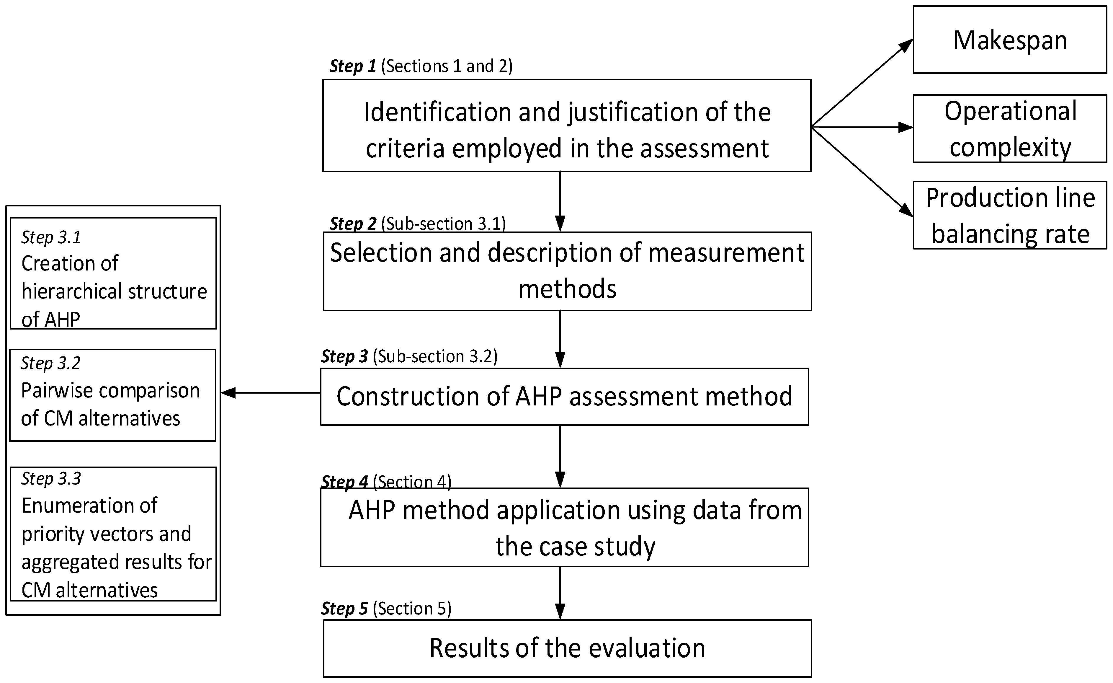
3. Methodological Framework

This section aims to describe in a nutshell the set of methods and overall procedure in chronological order and help the reader understand the context under which the research was conducted. In its first steps, the criteria or factors influencing the efficiency of CM systems have been mostly identified based on empirical findings and general knowledge of CM design, namely makespan and production line balancing rate. Similarly, measurement methods to quantify operational complexity have been chosen. Subsequently, the AHP method divided into three steps was used for the evaluation of individual CM alternatives. Summarily, the methodological framework of this research consists of five steps, which is illustrated in the figure below (Figure 1).

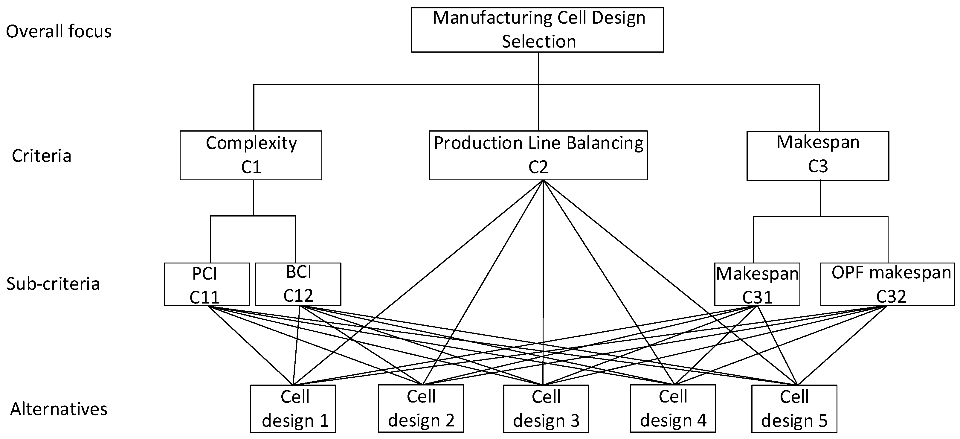
3.1. Indicators Used as Criteria to Assess Alternative CM Designs

3.1.1. Production Line Balancing Rate

The production line balancing rate (PLB) represents a measure of the average length of time of every cycle time in the working procedure on the processing line. It is equivalent to minimizing the number of workstations with a certain takt time [47]. It is expressed as [48]:

$$PLB=\frac{{\displaystyle {\sum }_{j=1}^n{t}_j}}{m\ast \max (T_i)} [\%],$$

(1)

where

• t_j stands for standard work time of the j-th job elements;
• n represents the number of the work elements;
• m represents the number of total lines in the production system;
• T_i represents the work time in the production line(s) (PL(s));
• max(T_i) represents the biggest line operating time.

3.1.2. Operational Complexity Indicators

There are several potential operational complexity indicators that can be applied to measure the operational complexity properties of manufacturing systems from different or similar perspectives (see, e.g., [49,50,51,52,53,54]). Two of them that suit the available data characterizing the benchmarked alternatives are further introduced.

• Process Complexity Indicator

This indicator, similar to the other concurrent complexity measures, is derived from Shannon’s information theory [55]. The process complexity indicator (PCI) is specified for the quantification of manufacturing process complexity, taking into account the operational complexities of individual machines. The PCI indicator is enumerated by using equation [54]:

$$PCI=-{\displaystyle \sum _{i=1}^M}{\displaystyle \sum _{j=1}^P}{\displaystyle \sum _{k=1}^O{p}_{\mathrm{ijk}}\cdot {\log }_2{p}_{\mathrm{ijk}}} [\mathrm{bits}],$$

(2)

where

• p_ijk stands for the probability that part j is processed due to operation k by individual machine i according to scheduling order;
• O is the number of operations according to parts production;
• P is the number of parts produced in the manufacturing process;
• M is the number of all machines of all types in the manufacturing process.

• Balanced Complexity Indicator

The balanced complexity indicator (BCI) takes into account the rate of mutual differences between the individual complexities of machines. This indicator expresses the variability of the partial complexities of workstations/machines and calculates the deviation of partial machine complexities from their mean value. It is calculated using the following formula [54]:

$$BCI=\frac{{\displaystyle \sum _{i=1}^{N}MC{I}_{i(\max )}^{}}-{\displaystyle \sum _{i=1}^{N}MC{I}_{i(\min )}}}{N} [\mathrm{bits}],$$

(3)

where

• MCI_i(max) represents the first N-max complexity values;
• MCI_i(min) represents the first N-min complexity values;
• N represents the number of max and min machine complexity values.

3.1.3. Makespan Indicators

For the purpose of calculating makespan, the scheduling algorithm to minimize the completion of n-jobs of m-machines is used. As known, there are many different algorithms for the given purpose. In this work, the freely available online software is utilized [56], and the following input data for this algorithm are collected:

• Processing times in minutes for each job, which are included in matrix m x n (Figure 2a);
• Number of transport batch (Figure 2b);
• Transport batch sizes for each job (Figure 2c);
• Sequences of individual jobs numbered by order (Figure 2d).

Its application in the first step requires that input data are presented in the form of a Microsoft Office Excel table and pasted into the input data window. A flowchart of how to generate makespan is shown in Figure 3.

As can be seen from Figure 3, makespans are enumerated assuming two scenarios. According to the first scenario, makespan is calculated for determined batch sizes, and for the second scenario, the one-piece flow (OPF) principle is applied, i.e., when the transport batch size for each job equals 1.

3.2. Description of AHP Method

Prior to describing the AHP method with the modified Saaty scale for a comparison of design alternatives in pairs using a multi-criteria decision-making approach, the five selected related AHP approaches are reported in

Table 1. Comparison of existing studies based on usage of AHP method.

Publication Title	Publication Characteristics
The use of AHP method for selection of supplier [57]	This article presents the general design of the model for the selection of a suitable supplier from three potential suppliers by the AHP method using Saaty’s point scale. The proposed model is applied in a manufacturing company.
A multi-Criteria decision support concept for selecting the optimal contractor [58]	This paper presents a decision support concept for selecting the optimal contractor. This concept increases the transparency of decision-making and the consistency of the decision-making process, and it has potential for application in similar decision-making problems.
Fuzzy AHP group decision analysis and its application for the evaluation of energy sources [59]	The evaluation of a multi-criteria decision problem by use of fuzzy logic is the main concern of this research. It considers the specific problem of the searching of energy alternatives and a proper evaluation of these alternatives in comparison with existing ones.
Modeling procedure for the selection of steel pipes supplier by applying fuzzy AHP method [60]	This work is focused on the evaluation and selection of suppliers by applying fuzzy multi-criteria analysis using the AHP method to choose the optimal supplier from five suppliers for the production of pre-insulated pipes. These suppliers are compared based on nine criteria, e.g., material cost, delivery time, transport distance, etc.
An application of analytic hierarchy process (AHP) in a real-world problem of store location selection [61]	This study presents a new store location selection problem of Carglass Turkey, which includes tangible and intangible criteria, and the analytic hierarchy process (AHP) was applied. The hierarchical model established for this problem may provide insight regarding location selection problems.
Simultaneous customers and supplier’s prioritization: an AHP based fuzzy inference decision support system (AHP-FIDSS) [62]	This research paper introduced a novel analytical hierarchical process-based fuzzy inference decision support system (AHP-FIDSS), which involves factor screening, hierarchical structure modeling, quantification of qualitative factors, and their conversion to quantitative values.

in order to point out the differences in the research addressed in our paper.

All of these AHP method applications are based on a subjective approach in mutual comparison of alternatives. On the contrary, the proposed procedure to find the most suitable cell design alternative(s) uses an objective approach of the pairwise comparison of cell design alternatives. In addition, it is necessary to select one of the possible methods in the application of the AHP method [63,64]. For the given purpose, the most accurate procedure seems to be that which consists of the following steps:

Step 1. Creation of hierarchical structure of AHP method. The hierarchical structure of the AHP method is created in the form of a diagram, where the criteria, sub-criteria, and CM alternatives are specified.

Step 2. Pairwise comparison of CM alternatives. All CM alternatives are pairwise benchmarked with respect to the criteria and sub-criteria. The pairwise comparison is provided in matrix form by comparing one CM alternative to another to determine the weights of importance. For this purpose, the proposed modified scale of relative importance is applied (see Section 4.3).

Step 3. Enumeration of priority vectors and aggregated results. The priorities are derived using the values of the principal right eigenvectors of the compared matrices. These priorities are expressed as absolute numbers bounded between 0 and 1, without units, and are calculated according to the so-called additive normalization method using the following simple procedure:

Sum each column values separately for each matrix, divide each element of the column with the sum of that column for each matrix, and compute the average of all elements in each row of all matrices to obtain the priority vector.

To obtain aggregated results, it is needed to summarize the determined priorities of all the individual indicators for each CM alternative. Then, the aggregated priorities are compared by ranking them in order from most to least important. Finally, the optimal CM alternative is selected.

4. A Practical Example

4.1. Description of Manufacturing Cell Designs Alternatives

This section aims to introduce five manufacturing cell alternatives for their mutual comparison in order to determine the optimal design. The CM alternative designs along with basic input data are taken from a case study by Yan and Irani [65]. The essential data from this case study include routing of parts (P) through machines (M), sequencing of parts by way of recording, operational times in minutes, and batch sizes for individual parts. The parts routings and operational times for all the parts are shown in Figure 4 (e.g., part P1 is firstly processed for 96 min on machine M1. It is subsequently machined for 36 min on machine M4, processed for 36 min on machine M8, and finally, it is machined for 72 min on machine M9).

The alternative designs that are depicted in Figure 5 can be divided into two groups: two-cell solutions (three design alternatives, i.e., Cell Designs 1–3) and three-cell solutions (two design alternatives, i.e., Cell Designs 4–5). The sequence of machines for each job is not violated in all the alternatives.

As can be seen in this figure, Cell Design 1 consists of two cells: 11 machines are located in the first cell, and 12 machines are located in the second cell. Parts P1–P4 and P7–P11 are processed in the first cell, and the rest of the parts marked as P12–P19 are processed only in the second cell. Parts P5 and P6 are partially processed in the second cell and finalized in the first cell.

Cell Design 2 contains 25 machines. There are 16 machines in the first cell and 9 machines in the second cell. Parts P1–P11 and P18 are machined in the first cell, and the rest of the parts are produced in the second cell.

Cell Design 3 is quite similar to Cell Design 2, except that machine M1 is eliminated in the second cell, and parts P15 and P16 are first produced in the first cell and subsequently finished in the second cell.

Cell Design 4 includes three cells with 8 machines in the first cell, 10 machines in the second cell, and 8 machines in the third cell. Parts marked as P1, P3, P7–P9, and P11 are machined in the first cell, while P3 is completed in the second cell. Parts P2, P4–P6, P10, P15, P16, and P18 are produced in the second cell, but P15 and P16 are finished in the third cell. Parts P12–P14, P17, and P19 are machined in the third cell.

Cell Design 5 is also divided into three cells. The first cell consists of 5 machines, 15 machines are located in the second cell, and 4 machines are placed in the third cell. P1, P3, P7–P9, and P11 are machined in the first cell, while P1, P3, and P7–P9 are completed in the second cell. P2, P4–6, P10, P14–P16, and P18 are produced in the second cell, while P15 and P16 are finalized in the third cell. P12, P13, P17, and P19 are machined only in the last cell.

4.2. Application of the Performance Indicators on Cell Designs

In this sub-section, the above-mentioned indicators are applied to the five CM alternatives. Obtained operational complexity values, makespans, and production line balancing rates are summarily shown in

Table 2. Enumerated results of all the criteria and sub-criteria.

Cell Designs	Makespan (min)	OPF Makespan (min)	PCI (bits)	BCI (bits)	PLB (%)
1	5926	3610	47.8	2.1	92.4 *
2	5014	3108	50.7	2.24	78.7
3	5049	3079	53.9	2.45	78.2
4	5438	3194	44.8 *	1.62 *	85.6
5	4650 *	2927 *	47.1	2.14	50.7

* Best obtained value.

.

The obtained values are further used as input data for the purpose of multi-criteria comparison applying the AHP method.

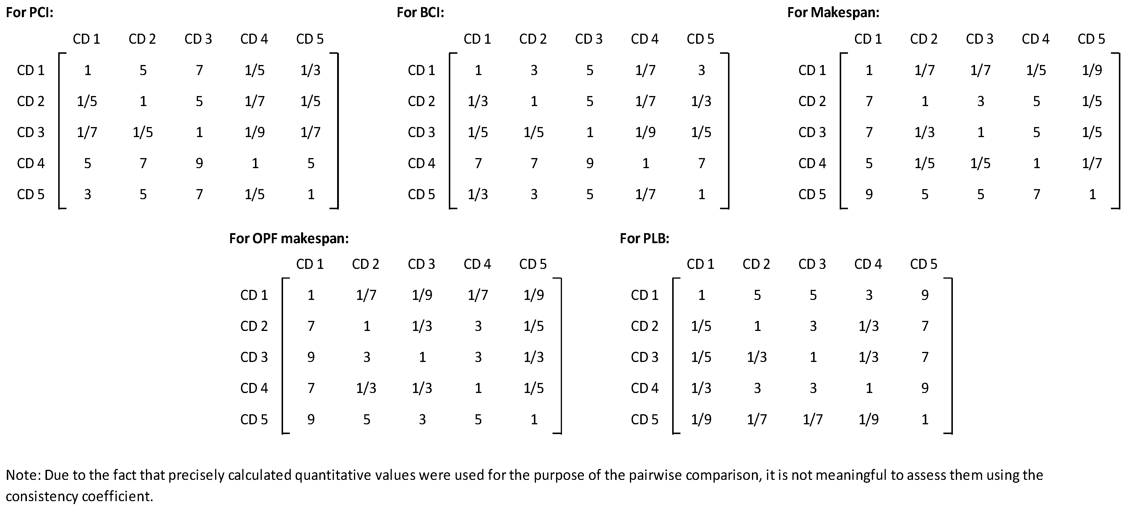
4.3. Assessment of Manufacturing Cell Designs Using AHP Method

Firstly, the hierarchical structure of the AHP method is created. The overall focus is aimed at the selection of the optimal manufacturing cell design(s) from the five cell design alternatives. For this purpose, these five alternatives are compared using the criteria shown in Figure 6.

Once the hierarchy is constructed, the alternatives are pairwise compared for each of the criteria based on the preferences using the scale of relative importance (see

Table 3. Scale of relative importance.

Scale	Numerical Rating	Explanation
Equal importance	1	Two alternatives contribute equally to the objective (0% difference)
Moderate importance	3	One alternative is slightly favored over another (no more than 25% difference)
Strong importance	5	One alternative is strongly favored over another (25–50% difference)
Very strong importance	7	One alternative is very strongly favored over another (50–75% difference)
Absolute importance	9	One alternative is absolutely favored over another (more than 75% difference)
Intermediate values	2, 4, 6, 8	When compromise is needed between two alternatives

Note: When comparing the best alternative with the worst alternative, the difference between them is maximally 100%. Based on this difference value, the percentages 25%, 50%, and/or 75% are proposed.

).

The performance of each cell design (CD) with regard to each criterion is indicated by the following pairwise comparison matrices, and at the same time, it is assumed that all criteria are equal to each other (see Figure 7).

Subsequently, the priority vectors are calculated according to the additive normalization method for all the criteria shown in

Table 4. Obtained priority vectors values for all the criteria.

Cell Designs	PCI	BCI	Makespan	OPF Makespan	PLB
1	0.15877167	0.175165699	0.029623447	0.027892418	0.476996214
2	0.072721123	0.085558568	0.221688177	0.148542569	0.148542569
3	0.029623447	0.03317987	0.15877167	0.245125107	0.101443692
4	0.517195582	0.580746424	0.072721123	0.101443692	0.245125107
5	0.221688177	0.125349438	0.517195582	0.476996214	0.027892418

.

Finally, the aggregated relative priorities from Table 4 are enumerated, which allows ranking CM alternatives, as shown in Figure 8.

As can be seen from Figure 8, Cell Design 4 is considered the optimal design.

5. Conclusions

Summarily, it can be stated that both of the three-cell solutions better satisfied the determined criteria of manufacturing cell design performance than all the three two-cell solutions. It can be empirically explained by this that cells practically represent modules, and a modular manufacturing layout design is better than an integral design.

Moreover, from the obtained results of the computational experiments, it can be noted that:

• According to both complexity indicators, the three-cell solutions are less complex than the two-cell solutions. The lower complexity of the three-cell designs against the two-cell designs can be comprehended in a way that the scheduling of cell designs with a higher number of cells is less complicated than in the case with a smaller number of cells. This statement comes from the fact the probability that parts are produced on given machines is higher than in the case of the CM design with a smaller number of cells;
• Based on the makespan results, the three-cell solutions better satisfied the minimization of the total time needed to finish all the jobs than the two-cell solutions;
• From the viewpoint of the PLB indicator, the two-cell solutions offer better balancing of machines than the three-cell solutions.

As mentioned, the case study was taken from the work of Yan and Irani [65], who compared two-cell solutions with three-cell solutions based on selected criteria such as the number of intra-cell flows and inter-cell flows, scheduling, etc., to point out the advantages and disadvantages of two-cell solutions and three-cell solutions. Our aim was to identify the optimal cell design solution(s) from the alternatives based on a multi-criteria decision-making approach, where five selected criteria were used. The main benefit of the used approach lies in the objective approach of the pairwise comparison of cell design alternatives in the decision-making process.

Related future research could be oriented to employ other criteria to assess manufacturing cells design performance in order to bring new findings for practitioners and researchers.

References

1. Qin, J.; Liu, Y.; Grosvenor, R. A Categorical Framework of Manufacturing for Industry 4.0 and Beyond. Procedia CIRP 2016, 52, 173–178. [Google Scholar] [CrossRef] [Green Version]
2. Tzafestas, E.S. A Study of Self-Organization in a Production Environment. In Advances in Manufacturing; Springer: London, UK, 1999; pp. 37–44. [Google Scholar]
3. Bortolini, M.; Galizia, F.G.; Mora, C.; Pilati, F. Reconfigurability in cellular manufacturing systems: A design model and mul-ti-scenario analysis. Int. J. Adv. Manuf. Technol. 2019, 104, 4387–4397. [Google Scholar] [CrossRef]
4. Modrak, V.; Pandian, R.S. Operations Management Research and Cellular Manufacturing Systems: Innovative Methods and Approaches; IGI Global: Hershey, PA, USA, 2012. [Google Scholar]
5. Huber, V.L.; Hyer, N.L. The human factor in cellular manufacturing. J. Oper. Manag. 1985, 5, 213–228. [Google Scholar] [CrossRef]
6. Kia, R.; Baboli, A.; Javadian, N.; Tavakkoli-Moghaddam, R.; Kazemi, M.; Khorrami, J. Solving a group layout design model of a dynamic cellular manufacturing system with alternative process routings, lot splitting and flexible reconfiguration by simulated annealing. Comput. Oper. Res. 2012, 39, 2642–2658. [Google Scholar] [CrossRef]
7. Renna, P.; Ambrico, M. Design and reconfiguration models for dynamic cellular manufacturing to handle market changes. Int. J. Comput. Integr. Manuf. 2015, 28, 170–186. [Google Scholar] [CrossRef]
8. Herrmann, J.W. A History of Production Scheduling. In Handbook of Production Scheduling; Springer: Boston, MA, USA, 2006; pp. 1–22. [Google Scholar]
9. Srimongkolkul, O.; Chongstitvatana, P. Minimizing Makespan Using Node Based Coincidence Algorithm in the Permutation Flowshop Scheduling Problem. In Industrial Engineering, Management Science and Applications; Springer: Berlin/Heidelberg, Germany, 2015; pp. 303–311. [Google Scholar]
10. Paul, S.K.; Azeem, A. Minimization of work in process inventory in hybrid flow shop scheduling using fuzzy logic. Int. J. Ind. Eng. Theory Appl. Pract. 2010, 17, 115–127. [Google Scholar]
11. Modrak, V.; Soltysova, Z. Batch Size Optimization of Multi-Stage Flow Lines in Terms of Mass Customization. Int. J. Simul. Model. 2020, 19, 219–230. [Google Scholar] [CrossRef]
12. Kuzgunkaya, O.; ElMaraghy, H.A. Assessing the structural complexity of manufacturing systems configurations. Int. J. Flex. Manuf. Syst. 2007, 18, 145–171. [Google Scholar] [CrossRef]
13. Modrak, V.; Marton, D. Configuration complexity assessment of convergent supply chain systems. Int. J. Gen. Syst. 2014, 43, 508–520. [Google Scholar] [CrossRef]
14. Trattner, A.; Hvam, L.; Forza, C.; Herbert-Hansen, Z.N.L. Product complexity and operational performance: A systematic literature review. CIRP J. Manuf. Sci. Technol. 2019, 25, 69–83. [Google Scholar] [CrossRef]
15. Calinescu, A. Manufacturing Complexity: An Integrative Information-Theoretic Approach. Ph.D. Dissertation, University of Oxford, Oxford, UK, 2002. [Google Scholar]
16. Park, K.; Kremer, G. The impact of complexity on manufacturing performance: A case study of the screwdriver product family. In Proceedings of the 2013 International Conference on Engineering Design, Seoul, Korea, 19–22 August 2013; The Design Society: Copenhagen, Denmark, 2013; Volume 3, pp. 141–150. [Google Scholar]
17. Bucki, R.; Suchánek, P. Comparative Simulation Analysis of the Performance of the Logistics Manufacturing System at the Operative Level. Complexity 2019, 2019, 7237585. [Google Scholar] [CrossRef]
18. Rogers, D.F.; Shafer, S.M. Measuring cellular manufacturing performance. Manuf. Res. Technol. 1995, 24, 147–165. [Google Scholar]
19. Flynn, B.B.; Jacobs, F.R. Applications and Implementation: An Experimental Comparison of Cellular (Group Technology) Layout with Process Layout. Decis. Sci. 1987, 18, 562–581. [Google Scholar] [CrossRef]
20. Morris, J.S.; Tersine, R.J. A Simulation Analysis of Factors Influencing the Attractiveness of Group Technology Cellular Layouts. Manag. Sci. 1990, 36, 1567–1578. [Google Scholar] [CrossRef]
21. Yuan, Y.; Xu, H.; Yang, J. A hybrid harmony search algorithm for the flexible job shop scheduling problem. Appl. Soft Comput. 2013, 13, 3259–3272. [Google Scholar] [CrossRef]
22. Liker, J.K. The Toyota Way; McGraw Hill: New York, NY, USA, 2004. [Google Scholar]
23. Kant, R.; Pattanaik, L.N.; Pandey, V. Framework for strategic implementation of cellular manufacturing in lean production environment. J. Manuf. Technol. Res. 2014, 6, 177. [Google Scholar]
24. Saraçoğlu, I.; Süer, G.A.; Gannon, P. Minimizing makespan and flowtime in a parallel multi-stage cellular manufacturing company. Robot. Comput. Manuf. 2021, 72, 102182. [Google Scholar] [CrossRef]
25. Belfiore, G.; Falcone, D.; Silvestri, L. Assembly line balancing techniques: Literature review of deterministic and stochastic methodologies. In Proceedings of the 17th International Conference on Modeling and Applied Simulation (MAS 2018), Budapest, Hungary, 17–19 September 2018; pp. 185–190. [Google Scholar]
26. Shinde, A.; More, D. Production Line Balancing: Is it a Balanced Act? Vikalpa 2015, 40, 242–247. [Google Scholar] [CrossRef] [Green Version]
27. Kottas, J.F.; Lau, H.-S. A cost oriented approach to stochastic line balancing. AIIE Trans. 1973, 5, 164–171. [Google Scholar] [CrossRef]
28. Moodie, C.L.; Young, H.H. A heuristic method of assembly line balancing assumptions of constant or variable work element times. J. Ind. Eng. 1965, 16, 23–29. [Google Scholar]
29. Kilbridge, M.D.; Wester, L. A heuristic method of assembly line balancing. J. Ind. Eng. 1961, 12, 292–298. [Google Scholar]
30. Helgeson, W.B.; Birnie, D.P. Assembly Line Balancing Using the Ranked Positional Weighting Technique. J. Ind. Eng. 1961, 12, 394–398. [Google Scholar]
31. Hazır, Ö.; Dolgui, A. Assembly line balancing under uncertainty Robust optimization models and exact solution method. Comput. Ind. Eng. 2013, 65, 261–267. [Google Scholar] [CrossRef]
32. Gurevsky, E.; Hazır, Ö.; Battaïa, O.; Dolgui, A. Robust balancing of straight assembly lines with interval task times. J. Oper. Res. Soc. 2013, 64, 1607–1613. [Google Scholar] [CrossRef]
33. Ponnambalam, S.G.; Aravindan, P.; Naidu, G.M. A comparative evaluation of assembly line balancing Heuristics. Int. J. Adv. Manuf. Technol. 1999, 15, 577–586. [Google Scholar] [CrossRef]
34. Özceylan, E.; Kalayci, C.B.; Güngör, A.; Gupta, S.M. Disassembly line balancing problem: A review of the state of the art and future directions. Int. J. Prod. Res. 2018, 57, 4805–4827. [Google Scholar] [CrossRef] [Green Version]
35. Hazır, Ö.; Dolgui, A. A Review on Robust Assembly Line Balancing Approaches. IFAC-Pap. 2019, 52, 987–991. [Google Scholar] [CrossRef]
36. Hon, K.K.B. Performance and Evaluation of Manufacturing Systems. CIRP Ann. 2005, 54, 139–154. [Google Scholar] [CrossRef]
37. Fredendall, L.D.; Gabriel, T.J. Manufacturing complexity: A quantitative measure. In Proceedings of the POMS Conference, Savannah, GA, USA, 4–7 April 2013. [Google Scholar]
38. Wiendahl, H.-P.; Scholtissek, P. Management and Control of Complexity in Manufacturing. CIRP Ann. 1994, 43, 533–540. [Google Scholar] [CrossRef]
39. Efthymiou, K.; Pagoropoulos, A.; Papakostas, N.; Mourtzis, D.; Chryssolouris, G. Manufacturing Systems Complexity Review: Challenges and Outlook. Procedia CIRP 2012, 3, 644–649. [Google Scholar] [CrossRef] [Green Version]
40. Suh, N.P. Complexity: Theory and Applications; Oxford University Press: New York, NY, USA, 2005. [Google Scholar]
41. Zhang, Z. Modeling complexity of cellular manufacturing systems. Appl. Math. Model. 2011, 35, 4189–4195. [Google Scholar] [CrossRef]
42. Tainter, J.A. Social complexity and sustainability. Ecol. Complex. 2006, 3, 91–103. [Google Scholar] [CrossRef]
43. ElMaraghy, W.; ElMaraghy, H.; Tomiyama, T.; Monostori, L. Complexity in engineering design and manufacturing. CIRP Ann. 2012, 61, 793–814. [Google Scholar] [CrossRef]
44. Delgoshaei, A.; Gomes, C. A multi-layer perceptron for scheduling cellular manufacturing systems in the presence of unreliable machines and uncertain cost. Appl. Soft Comput. 2016, 49, 27–55. [Google Scholar] [CrossRef]
45. Solimanpur, M.; Elmi, A. A tabu search approach for cell scheduling problem with makespan criterion. Int. J. Prod. Econ. 2013, 141, 639–645. [Google Scholar] [CrossRef]
46. Saeed, K.; Dvorský, J. Computer Information Systems and Industrial Management, Proceedings of the 19th International Conference, CISIM 2020, Bialystok, Poland, 16–18 October 2020; Springer Nature Switzerland AG: Cham, Switzerland, 2020. [Google Scholar]
47. Hu, X.; Zhang, Y.; Zeng, N.; Wang, D. A Novel Assembly Line Balancing Method Based on PSO Algorithm. Math. Probl. Eng. 2014, 2014, 743695. [Google Scholar] [CrossRef]
48. Bhattacharjee, T.K.; Sahu, S. Complexity of single model assembly line balancing problems. Eng. Costs Prod. Econ. 1990, 18, 203–214. [Google Scholar] [CrossRef]
49. ElMaraghy, H.A.; Kuzgunkaya, O.; Urbanic, R.J. Manufacturing Systems Configuration Complexity. CIRP Ann. 2005, 54, 445–450. [Google Scholar] [CrossRef]
50. Dolgui, A.; Kovalev, S. Scenario based robust line balancing: Computational complexity. Discret. Appl. Math. 2012, 160, 1955–1963. [Google Scholar] [CrossRef]
51. Sivadasan, S.; Efstathiou, J.; Calinescu, A.; Huatuco, L.H. Advances on measuring the operational complexity of supplier–customer systems. Eur. J. Oper. Res. 2006, 171, 208–226. [Google Scholar] [CrossRef]
52. Isik, F. An entropy-based approach for measuring complexity in supply chains. Int. J. Prod. Res. 2009, 48, 3681–3696. [Google Scholar] [CrossRef] [Green Version]
53. Zhang, Z. Manufacturing complexity and its measurement based on entropy models. Int. J. Adv. Manuf. Technol. 2012, 62, 867–873. [Google Scholar] [CrossRef]
54. Modrak, V.; Soltysova, Z. Development of operational complexity measure for selection of optimal layout design alternative. Int. J. Prod. Res. 2018, 56, 7280–7295. [Google Scholar] [CrossRef]
55. Shannon, C.E. A Mathematical Theory of Communication. Bell Syst. Tech. J. 1948, 27, 623–656. [Google Scholar] [CrossRef]
56. Online Computing Software. Available online: http://paseka.epizy.com/ (accessed on 5 December 2021).
57. Hruška, R.; Průša, P.; Babić, D. The use of AHP method for selection of supplier. Transport 2014, 29, 195–203. [Google Scholar] [CrossRef] [Green Version]
58. Marović, I.; Perić, M.; Hanak, T. A Multi-Criteria Decision Support Concept for Selecting the Optimal Contractor. Appl. Sci. 2021, 11, 1660. [Google Scholar] [CrossRef]
59. Meixner, O. Fuzzy AHP group decision analysis and its application for the evaluation of energy sources. In Proceedings of the 10th International Symposium on the Analytic Hierarchy/Network Process, Pittsburgh, PA, USA, 29 July–1 August 2009; Volume 29, pp. 2–16. [Google Scholar]
60. Zavadskas, E.K.; Turskis, Z.; Stević, Ž.; Mardani, A. Modelling Procedure for the Selection of Steel Pipes Supplier by Applying Fuzzy AHP Method. Oper. Res. Eng. Sci. Theory Appl. 2020, 3, 39–53. [Google Scholar] [CrossRef]
61. Koç, E.; Burhan, H.A. An application of analytic hierarchy process (AHP) in a real world problem of store location selection. Adv. Manag. Appl. Econ. 2015, 5, 41–50. [Google Scholar]
62. Imran, M.; Agha, M.H.; Ahmed, W.; Sarkar, B.; Ramzan, M.B. Simultaneous Customers and Supplier’s Prioritization: An AHP-Based Fuzzy Inference Decision Support System (AHP-FIDSS). Int. J. Fuzzy Syst. 2020, 22, 2625–2651. [Google Scholar] [CrossRef]
63. Saaty, T.L. A scaling method for priorities in hierarchical structures. J. Math. Psychol. 1977, 15, 234–281. [Google Scholar] [CrossRef]
64. Saaty, T.L. The Analytic Hierarchy Process; McGraw-Hill: New York, NY, USA, 1980. [Google Scholar]
65. Yan, L.; Irani, S.A. Classroom Tutorial on the Design of a Cellular Manufacturing System. In Handbook of Cellular Manufacturing Systems; Irani, S.A., Ed.; John Wiley & Sons, Inc.: Hoboken, NJ, USA, 1999. [Google Scholar]
Figure 1. Overall research procedure in chronological order (Section 1, Section 2, Section 3, Section 4 and Section 5).
Applsci 12 00854 g001
Figure 2. Table format for insertion of input data, (a) processing times in minutes for each job, which are included in matrix m x n, (b) number of transport batch, (c) transport batch sizes for each job, (d) sequences of individual jobs numbered by order.
Applsci 12 00854 g002
Figure 3. Software flowcharts with acquired data.
Applsci 12 00854 g003
Figure 4. Sequences of machines for each job/part.
Applsci 12 00854 g004
Figure 5. Cell design alternatives and their material flows.
Applsci 12 00854 g005
Figure 6. Hierarchical structure of the AHP method for selection of an optimal manufacturing cell.
Applsci 12 00854 g006
Figure 7. Obtained values of pairwise comparison matrices for Cell Designs 1–5.
Applsci 12 00854 g007
Figure 8. Final comparison of cell designs.
Applsci 12 00854 g008