Article

Rapid-Erection Backstepping Tracking Control for Electrohydraulic Lifting Mechanisms of Launcher Systems

1
Department of Aerospace Engineering, Beijing Institute of Technology, Beijing 100081, China
2
School of Mechanical Engineering, Nanjing University of Science and Technology, Nanjing 210094, China
*
Author to whom correspondence should be addressed.
Appl. Sci. 2022, 12(2), 893; https://doi.org/10.3390/app12020893
Submission received: 11 December 2021 / Revised: 11 January 2022 / Accepted: 13 January 2022 / Published: 16 January 2022
(This article belongs to the Special Issue Recent Advances in Flow Control)

Abstract

:
Uncertainties and disturbances widely exist in electrohydraulic lifting mechanisms of launcher systems, which may worsen the rapid-erection tracking accuracy and even make the system unstable. To deal with the issue, an asymptotic tracking control framework is developed for electrohydraulic lifting mechanisms of launcher systems. Firstly, the dynamic equations and state-space forms of the electrohydraulic lifting mechanism are modeled. Based on the system model, a nonlinear rapid-erection robust controller is constructed to achieve the improvement of the system control performance, in which a nonlinear feedback term is employed to remove the effects of uncertainties and disturbances on tracking performance. Compared to the existing results, the asymptotic tracking stability of the closed-loop system can be assured based on the Lyapunov theory analysis. In the end, the simulation example of an actual electrohydraulic lifting mechanism of the launcher system is done to validate the effectiveness with the proposed controller.

1. Introduction

Electrohydraulic lifting mechanisms have been increasingly used in launcher systems [1,2,3,4,5] in terms of their merits containing large force/torque output, high response and small size-to-power ratio. Nevertheless, due to strong nonlinearities (i.e., flow nonlinearity, friction nonlinearity and mechanism nonlinearity) and unmodeled uncertainties (i.e., unmodeled friction, parametric uncertainties and extern disturbances) in electrohydraulic lifting mechanisms of launcher systems, the achievement of high-accuracy tracking control for electrohydraulic lifting mechanisms of launcher systems is challenging [6,7,8,9,10]. Thus, to address this issue and achieve the improvement of control performance for electrohydraulic lifting mechanisms of launcher systems, it is necessary to investigate some efficient control methods.
In the last few years, a lot of advanced controllers have been adopted to attain high-performance tracking for electrohydraulic actuator systems. Feedback linearization control found in [11,12] was used to dispose of dynamic nonlinearities by utilizing the feedforward compensation method. To handle parametric uncertainties in electrohydraulic actuator systems, adaptive control was employed in [13], while it could not suppress unmodeled disturbances [14]. Adaptive robust control investigated in [14] could deal with parametric uncertainties and extern disturbances simultaneously and has been broadly adopted in practice [15,16,17,18,19]. Nonetheless, the theoretical analysis of this controller shows that bounded tracking performance was achieved in the presence of time-variant disturbances. By integrating a robust integral of the sign of the error feedback (RISE) [20] and backstepping method, a RISE-based backstepping controller was developed for hydraulic systems in [21,22] to get an asymptotic stability while existing smooth disturbances. In addition, sliding mode control was used in [23] to suppress disturbances and improve control performance for hydraulic systems. A super-twisting controller (STC) is proposed in [24] to attain a finite-time stability. However, to suppress heavy disturbances, the achievable tracking performance in [21,22,23,24] was pledged in a high-frequency/high-gain feedback way. That is, by this way, high-frequency dynamics might be stimulated and then the system might get unstable.
To remove the effect of strong disturbances on control accuracy and improve the tracking performance, many disturbance estimators/observers have been developed. An extended state observer (ESO) in [25] was employed to estimate mismatched and matched disturbances and compensate them in a feedforward way. However, the asymptotic control performance of the system would be destroyed while facing time-variant disturbances. An unknown system dynamic estimator [26] was employed to dispose of unknown dynamics and modeling uncertainties for servo mechanisms, which only pledged a bounded stability when existing changing dynamics. Recently, an efficient sliding mode observer developed in [27] was used to dispose of pressure dynamics and force dynamics in hydraulic systems. In this way, an asymptotic stability was expected. However, the existence of the standard sign function could lead to serve chattering and even make the system unstable. Moreover, a distributed control framework presented in [28,29] were adopted to dispose of various uncertainties for robot arms, which achieved the improvement of the control performance. In addition, compared to the above-mentioned control approaches for hydraulic actuators, the rapid-erection controller design of the electrohydraulic lifting mechanism in launcher systems considered in this paper is more complex due to its inherent mechanism nonlinearities. Consequently, how to design an asymptotic rapid-erection robust control method for the electrohydraulic lifting mechanism of the launcher system still is an open issue and deserve to study.
In this paper, a rapid-erection backstepping tracking controller for the electrohydraulic lifting mechanism of the launcher system with asymptotic stability is developed. To deal with the work, firstly, the dynamic equations and state-space forms of the electrohydraulic lifting mechanism of the launcher system are modeled. Based on the state-space system function, a nonlinear robust controller is constructed to achieve the improvement of the system control performance, in which a nonlinear feedback term is employed to remove the effects of uncertainties and disturbances on tracking performance. In the meanwhile, based on the Lyapunov theory analysis, the asymptotic tracking stability of the closed-loop system can be assured. In the end, the simulation example of an actual electrohydraulic lifting mechanism of the launcher system is carried out to validate the effectiveness with the proposed controller.
The main contributions of this article include the following aspects. (1) A rapid-erection backstepping robust control with asymptotic tracking performance is developed for the electrohydraulic lifting mechanism of launcher systems subject to mechanism nonlinearities, friction nonlinearities and time-variant disturbances. (2) A continuous nonlinear feedback term is adopted to strengthen the robustness of the system and realize the improvement of the control accuracy. (3) The control merits of the presented control method are tested by corresponding simulation results when compared to the existing controllers containing feedback linearization control in [11], robust control and proportional-integral control.
The arrangement of this paper is provided as follows: System modeling of the electrohydraulic lifting mechanism of the launcher system can be seen in Section 2. The controller design and its theoretical analysis are provided in Section 3. Simulation results are found from Section 4. The simulation results uncover the validity of the developed control method. The conclusion is made in Section 5.

2. System Modeling

The considered electrohydraulic lifting mechanism with two motion states can be seen from Figure 1, where one state of the lifting mechanism lies in a horizontal position and the other lies in any motion position.

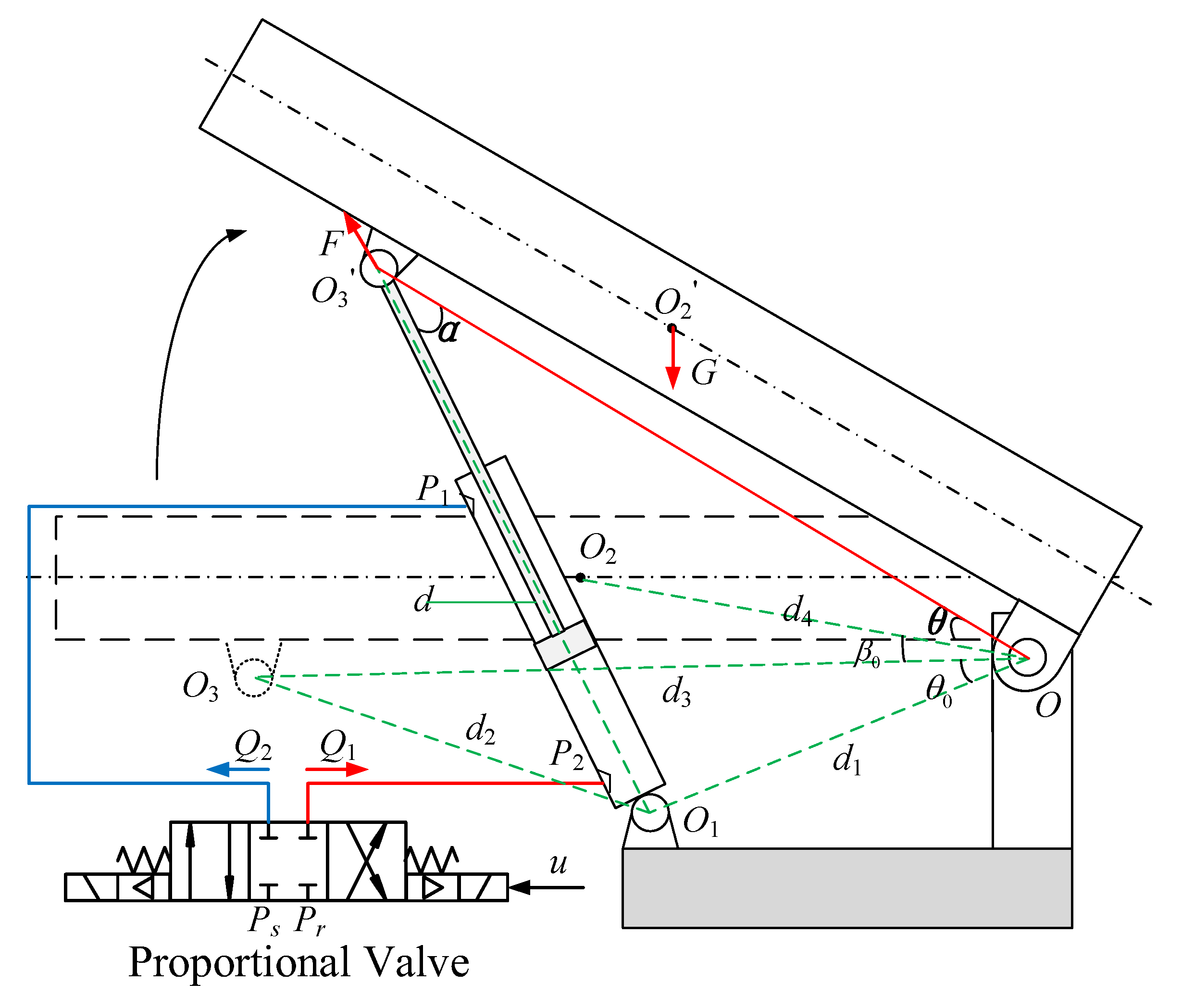
2.1. The Dynamics of the Lifting Mechanism

As observer from Figure 1, O denotes the gyration center; O1 and O3 stand for rotation centers of the lower and upper ears of the hydraulic cylinder severally; O2 denotes the barycenter of the lifting mechanism; θ stands for the rotary angle of the lifting mechanism arm, whose range is 0~90°; u stands for the control input; Q1 and Q2 stand for the return flow and supplied flow of the hydraulic cylinder severally; Pr and Ps stand for the return pressure and supply pressure severally; G and F stand for the force acting on the arm and the gravity of the arm severally. In addition, define OO1 = d1, OO2 = d4, OO3 = d3, O1O3 = d2, O1O3′ = d, ∠O3OO2′ = θ , ∠O3OO1 = θ 0 , ∠O3OO2 = β 0 and ∠O1O3′O = α .
The dynamics of the lifting mechanism is expressed by
J θ ¨ = F d 3 sin ( α ) m g d 4 cos ( β 0 + θ ) A f S f ( θ ˙ ) B θ ˙ + Δ ( t )
where J stands for the rotary inertia; m stands for the mass of the lifting mechanism arm; F = A1P1A2P2, where P1 and P2 stand for the pressure values of two chambers in the hydraulic cylinder severally, A1 and A2 stand for the effective areas of two chambers in the hydraulic cylinder severally; Af and Sf stand for the amplitude and approximated shape function of the Coulomb friction; B stands for the viscous friction coefficient; Δ ( t ) stands for the unmodelled disturbances.
By applying the cosine law, it yields
d = d 1 2 + d 3 2 2 d 1 d 3 cos ( θ 0 + θ )
Defining the cylinder displacement as x s = d d 2 , one has
x s θ = d 1 d 3 sin ( θ 0 + θ ) d 1 2 + d 3 2 2 d 1 d 3 cos ( θ 0 + θ )
Based on the sine law, there is
d 1 sin ( α ) = d sin ( θ 0 + θ )
Involving the Equations (1)–(4), it is easy to obtain that
J θ ¨ = x s θ ( A 1 P 1 A 2 P 2 ) m g d 4 cos ( β 0 + θ ) A f S f ( θ ˙ ) B θ ˙ + Δ ( t )

2.2. The Dynamics of the Electrohydraulic Actuator

Taking the oil compressibility into consideration, the pressure dynamics of the electrohydraulic actuator is written as [30,31]
V 1 β e P ˙ 1 = Q 1 A 1 x s θ θ ˙ C ( P 1 P 2 ) + q 1 ( t ) V 2 β e P ˙ 2 = Q 2 + A 2 x s θ θ ˙ + C ( P 1 P 2 ) q 2 ( t )
where V1 = V01 + A1xs and V2 = V02A2xs stand for the volumes of the two chambers severally; V01 and V02 stand for the original volumes of the two chambers severally; β e stands for the effective oil bulk modulus; C stands for the internal leakage coefficient; q1(t) and q2(t) stand for the unmodelled disturbances.
Given that a high-performance proportional valve is utilized in this paper, the servo valve dynamics can be omitted. Consequently, the control input u is assumed to be proportional to the valve spool displacement. The flows Q1 and Q2 thus are modeled as [32]
Q 1 = k t u s i g ( u ) P s P 1 + s i g ( u ) P 1 P r Q 2 = k t u s i g ( u ) P 2 P r + s i g ( u ) P s P 2
where kt stands for the flow gain; sig(u) is defined as
s i g ( u ) = 1 , i f   u 0 0 , i f   u < 0
From (6), it has
A 1 P ˙ 1 A 2 P ˙ 2 = A 1 β e V 1 Q 1 A 1 x s θ θ ˙ C ( P 1 P 2 ) + q 1 ( t ) A 2 β e V 2 Q 2 + A 2 x s θ θ ˙ + C ( P 1 P 2 ) q 2 ( t ) = β e ( A 1 V 1 Q 1 + A 2 V 2 Q 2 ) β e ( A 1 2 V 1 + A 2 2 V 2 ) x s θ θ ˙ β e ( A 1 V 1 + A 2 V 2 ) C ( P 1 P 2 ) + β e A 1 V 1 q 1 ( t ) + A 2 V 2 q 2 ( t )
Putting (7) into (9), it leads to
A 1 P ˙ 1 A 2 P ˙ 2 = β e k t ( A 1 V 1 s 1 + A 2 V 2 s 2 ) u β e ( A 1 2 V 1 + A 2 2 V 2 ) x s θ θ ˙ β e ( A 1 V 1 + A 2 V 2 ) C ( P 1 P 2 ) + β e A 1 V 1 q 1 ( t ) + A 2 V 2 q 2 ( t )
in which
s 1 = s i g ( u ) P s P 1 + s i g ( u ) P 1 P r s 2 = s i g ( u ) P 2 P r + s i g ( u ) P s P 2

2.3. System State-Space Form

Constructing the state variables x = x 1 ; x 2 ; x 3 = θ ; θ ˙ ; A 1 P 1 A 2 P 2 , the system state-space form by using (5) and (10) is
x ˙ 1 = x 2 J x ˙ 2 = x s x 1 x 3 m g d 4 cos ( β 0 + x 1 ) A f S f ( x 2 ) B x 2 + Δ ( t ) x ˙ 3 = φ 1 u φ 2 + q ( t )
in which
φ 1 = β e k t ( A 1 V 1 s 1 + A 2 V 2 s 2 ) φ 2 = β e ( A 1 2 V 1 + A 2 2 V 2 ) x s x 1 x 2 + β e ( A 1 V 1 + A 2 V 2 ) C ( P 1 P 2 ) q ( t ) = β e A 1 V 1 q 1 ( t ) + A 2 V 2 q 2 ( t )
We attempt to let the tracking error converge to zero by using the developed control approach on basis of two assumptions:
Assumption 1.
The terms Δ ( t ) and q ( t ) in (12) satisfy.
Δ ( t ) c 1 , q ( t ) c 2
where c i ( i = 1 , 2 ) are known positive constants.
Assumption 2.
The reference trajectory x 1 d 3 and is bounded.

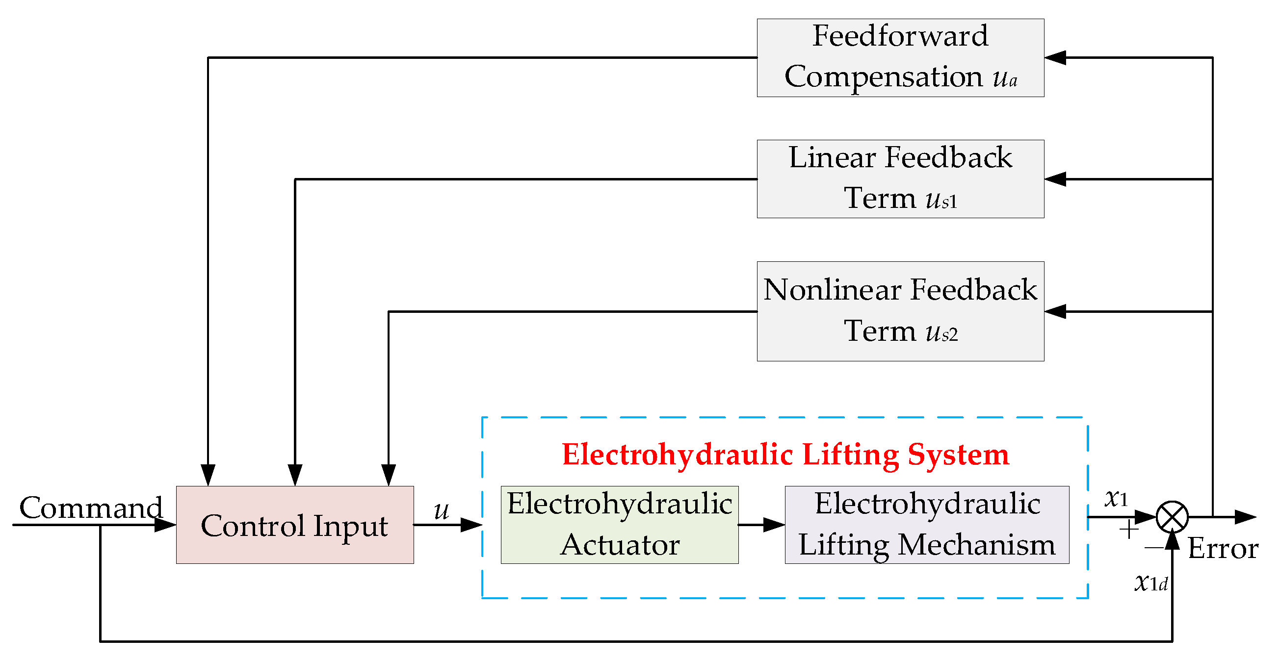
3. Controller Design

3.1. Controller Design

For simplifying the controller development, by using the backstepping method, several variables are designed as below
ξ 1 = x 1 x 1 d ξ 2 = k 1 ξ 1 + ξ ˙ 1 = x 2 x 2 d x 2 d = x ˙ 1 d k 1 ξ 1 ξ 3 = x 3 x 3 d
where k 1 is non-negative; ξ 1 stands for the tracking error; x 2 d denotes the virtual control law of the state x2; ξ 2 stands for the discrepancy between the actual state x2 and the virtual control x 2 d ; x 3 d denotes the virtual control law of the state x3; ξ 3 stands for the discrepancy between the actual state x3 and the virtual control x 3 d .
Step 1: On basis of the Formulas (12) and (15) and differentiating ξ 2 , there is
J ξ ˙ 2 = J x ˙ 2 J x ˙ 2 d = x s x 1 x 3 m g d 4 cos ( β 0 + x 1 ) A f S f ( x 2 ) B x 2 + Δ ( t ) J x ˙ 2 d = x s x 1 ξ 3 + x 3 d m g d 4 cos ( β 0 + x 1 ) A f S f ( x 2 ) B x 2 + Δ ( t ) J x ˙ 2 d
From (16), the virtual control x 3 d is constructed as
x 3 d = x s x 1 1 ( x 3 d a + x 3 d s ) , x 3 d s = x 3 d s 1 + x 3 d s 2 x 3 d a = m g d 4 cos ( β 0 + x 1 ) + A f S f ( x 2 ) + B x 2 + J x ˙ 2 d ξ 1 x 3 d s 1 = k 2 ξ 2 , x 3 d s 2 = k 2 s ξ 2 c 1 2 k 2 s ξ 2 c 1 tanh ( ξ 2 / b 1 ( t ) ) + b 1 ( t )
where k 2 and k 2 s are positive constants; b 1 ( t ) > 0 and 0 t b 1 ( v ) d v τ 1 < + , with τ 1 being positive.
In (17), x 3 d a stands for the model-based feedforward compensation term that is utilized to achieve accurate model compensation and then improve the tracking performance. x 3 d s consisting of the linear feedback term x 3 d s 1 and the nonlinear feedback term x 3 d s 2 denotes the robust control law that is employed to remove the impact of external disturbances on the tracking performance.
Putting (17) into (16), one has
J ξ ˙ 2 = x s x 1 ξ 3 + x 3 d a + x 3 d s + m g d 4 cos ( β 0 + x 1 ) A f S f ( x 2 ) B x 2 + Δ ( t ) J x ˙ 2 d = x s x 1 ξ 3 + m g d 4 cos ( β 0 + x 1 ) + A f S f ( x 2 ) + B x 2 + J x ˙ 2 d ξ 1 k 2 ξ 2 + x 3 d s 2 + m g d 4 cos ( β 0 + x 1 ) A f S f ( x 2 ) B x 2 + Δ ( t ) J x ˙ 2 d = x s x 1 ξ 3 ξ 1 k 2 ξ 2 k 2 s ξ 2 c 1 2 k 2 s ξ 2 c 1 tanh ( ξ 2 / b 1 ( t ) ) + b 1 ( t ) + Δ ( t )
Step 2: On basis of the Formulas (12) and (15) and differentiating ξ 3 , there is
ξ ˙ 3 = x ˙ 3 x ˙ 3 d = φ 1 u φ 2 + q ( t ) x ˙ 3 d
Hence, the controller input is designed as below
u = ( u a + u s ) φ 1 , u s = u s 1 + u s 2 u a = φ 2 + x ˙ 3 d x s x 1 ξ 2 u s 1 = k 3 ξ 3 , u s 2 = k 3 s ξ 3 c 2 2 k 3 s ξ 3 c 2 tanh ( ξ 3 / b 2 ( t ) ) + b 2 ( t )
where k 3 and k 3 s are positive constants; b 2 ( t ) > 0 and 0 t b 2 ( v ) d v τ 2 < + , with τ 2 being positive.
In (20), u a stands for the model-based feedforward compensation term that is utilized to achieve accurate model compensation and then improve the tracking performance. u s consisting of the linear feedback term u s 1 and the nonlinear feedback term u s 2 denotes the robust control law that is employed to remove the impact of external disturbances on the tracking performance.
Putting (17) into (16), one has
ξ ˙ 3 = u a + u s φ 2 + q ( t ) x ˙ 3 d = φ 2 + x ˙ 3 d x s x 1 ξ 2 k 3 ξ 3 k 3 s ξ 3 c 2 2 k 3 s ξ 3 c 2 tanh ( ξ 3 / b 2 ( t ) ) + b 2 ( t ) φ 2 + q ( t ) x ˙ 3 d = k 3 ξ 3 x s x 1 ξ 2 k 3 s ξ 3 c 2 2 k 3 s ξ 3 c 2 tanh ( ξ 3 / b 2 ( t ) ) + b 2 ( t ) + q ( t )
The control diagram of the lifting mechanism is provided in Figure 2 below.

3.2. Stability Analysis

The main result in this paper is reduced as below.
Theorem 1.
With the Assumptions 1 and 2 and the control law (20), by picking up the proper control parameters k 1 , k 2 , k 2 s , k 3 and k 3 s ,it can be inferred that all signals are bounded in the closed loop system and asymptotic tracking performance is then realized, i.e., ξ 1 0 as t + .
Proof of Theorem 1.
Construct a Lyapunov function as below
L = 1 2 ξ 1 2 + 1 2 ξ 2 2 + 1 2 ξ 3 2
According to (15), (18) and (21), the derivative of L is
L ˙ = ξ 1 ξ ˙ 1 + ξ 2 ξ ˙ 2 + ξ 3 ξ ˙ 3 = ξ 1 ( ξ 2 k 1 ξ 1 ) + ξ 2 x s x 1 ξ 3 ξ 1 k 2 ξ 2 k 2 s ξ 2 c 1 2 k 2 s ξ 2 c 1 tanh ( ξ 2 / b 1 ( t ) ) + b 1 ( t ) + Δ ( t ) + ξ 3 k 3 ξ 3 x s x 1 ξ 2 k 3 s ξ 3 c 2 2 k 3 s ξ 3 c 2 tanh ( ξ 3 / b 2 ( t ) ) + b 2 ( t ) + q ( t ) = k 1 ξ 1 2 + ξ 1 ξ 2 k 2 ξ 2 2 + x s x 1 ξ 2 ξ 3 ξ 1 ξ 2 + k 2 s ξ 2 2 c 1 2 k 2 s ξ 2 c 1 tanh ( ξ 2 / b 1 ( t ) ) + b 1 ( t ) + ξ 2 Δ ( t ) x s x 1 ξ 2 ξ 3 k 3 ξ 3 2 + k 3 s ξ 3 2 3 c 2 2 k 3 s ξ 3 c 2 tanh ( ξ 3 / b 2 ( t ) ) + b 2 ( t ) + ξ 3 q ( t ) = k 1 ξ 1 2 k 2 ξ 2 2 + k 2 s ξ 2 2 c 1 2 k 2 s ξ 2 c 1 tanh ( ξ 2 / b 1 ( t ) ) + b 1 ( t ) + ξ 2 Δ ( t ) k 3 ξ 3 2 + k 3 s ξ 3 2 3 c 2 2 k 3 s ξ 3 c 2 tanh ( ξ 3 / b 2 ( t ) ) + b 2 ( t ) + ξ 3 q ( t )
Noting that
0 ξ 2 tanh ξ 2 / b 1 ( t ) ξ 2 0 ξ 3 tanh ξ 3 / b 2 ( t ) ξ 3
It results in
k 2 s ξ 2 2 c 1 2 k 2 s ξ 2 c 1 tanh ( ξ 2 / b 1 ( t ) ) + b 1 ( t ) k 2 s ξ 2 2 c 1 2 k 2 s ξ 2 c 1 + b 1 ( t ) k 3 s ξ 3 2 3 c 2 2 k 3 s ξ 3 c 2 tanh ( ξ 3 / b 2 ( t ) ) + b 2 ( t ) k 3 s ξ 3 2 3 c 2 2 k 3 s ξ 3 c 2 + b 2 ( t )
Substituting (25) into (23), one has
L ˙ k 1 ξ 1 2 k 2 ξ 2 2 + k 2 s ξ 2 2 c 1 2 k 2 s ξ 2 c 1 + b 1 ( t ) + ξ 2 Δ ( t ) k 3 ξ 3 2 + k 3 s ξ 3 2 3 c 2 2 k 3 s ξ 3 c 2 + b 2 ( t ) + ξ 3 q ( t ) k 1 ξ 1 2 k 2 ξ 2 2 k 2 s ξ 2 2 c 1 2 k 2 s ξ 2 c 1 + b 1 ( t ) + ξ 2 c 1 k 3 ξ 3 2 + k 3 s ξ 3 2 3 c 2 2 k 3 s ξ 3 c 2 + b 2 ( t ) + ξ 3 c 2 k 1 ξ 1 2 k 2 ξ 2 2 + ξ 2 c 1 b 1 ( t ) k 2 s ξ 2 c 1 + b 1 ( t ) k 3 ξ 3 2 + ξ 3 c 2 b 2 ( t ) k 3 s ξ 3 c 2 + b 2 ( t )
Considering b 1 ( t ) > 0 and b 2 ( t ) > 0 , it leads to
L ˙ < k 1 ξ 1 2 k 2 ξ 2 2 + ξ 2 c 1 b 1 ( t ) k 2 s ξ 2 c 1 k 3 ξ 3 2 + ξ 3 c 2 b 2 ( t ) k 3 s ξ 3 c 2 k 1 ξ 1 2 k 2 ξ 2 2 + b 1 ( t ) k 2 s k 3 ξ 3 2 + b 2 ( t ) k 3 s
Then, it is easy to get
L ˙ κ ( ξ 1 2 + ξ 2 2 + ξ 3 2 ) + b 1 ( t ) k 2 s + b 2 ( t ) k 3 s κ L 1 + b 1 ( t ) k 2 s + b 2 ( t ) k 3 s
where κ = min { k 1 , k 2 , k 3 } , L 1 ξ 1 2 + ξ 2 2 + ξ 3 2 .
Integrating two sides of the inequality (28), one gets
L t + 0 t κ L 1 ν d ν L 0 + 0 t b 1 ( ν ) k 2 s + b 2 ( ν ) k 3 s d ν L 0 + τ 1 k 2 s + τ 2 k 3 s
Hence, L L , L 1 L 2 and the boundness of all the system signals holds. Thus, it is reduced that L 1 is uniformly continuous. By applying the Barbalat’s lemma [33], L 1 0 as t . Consequently, the tracking error asymptotically converges to zero and, thus, Theorem 1 holds. □

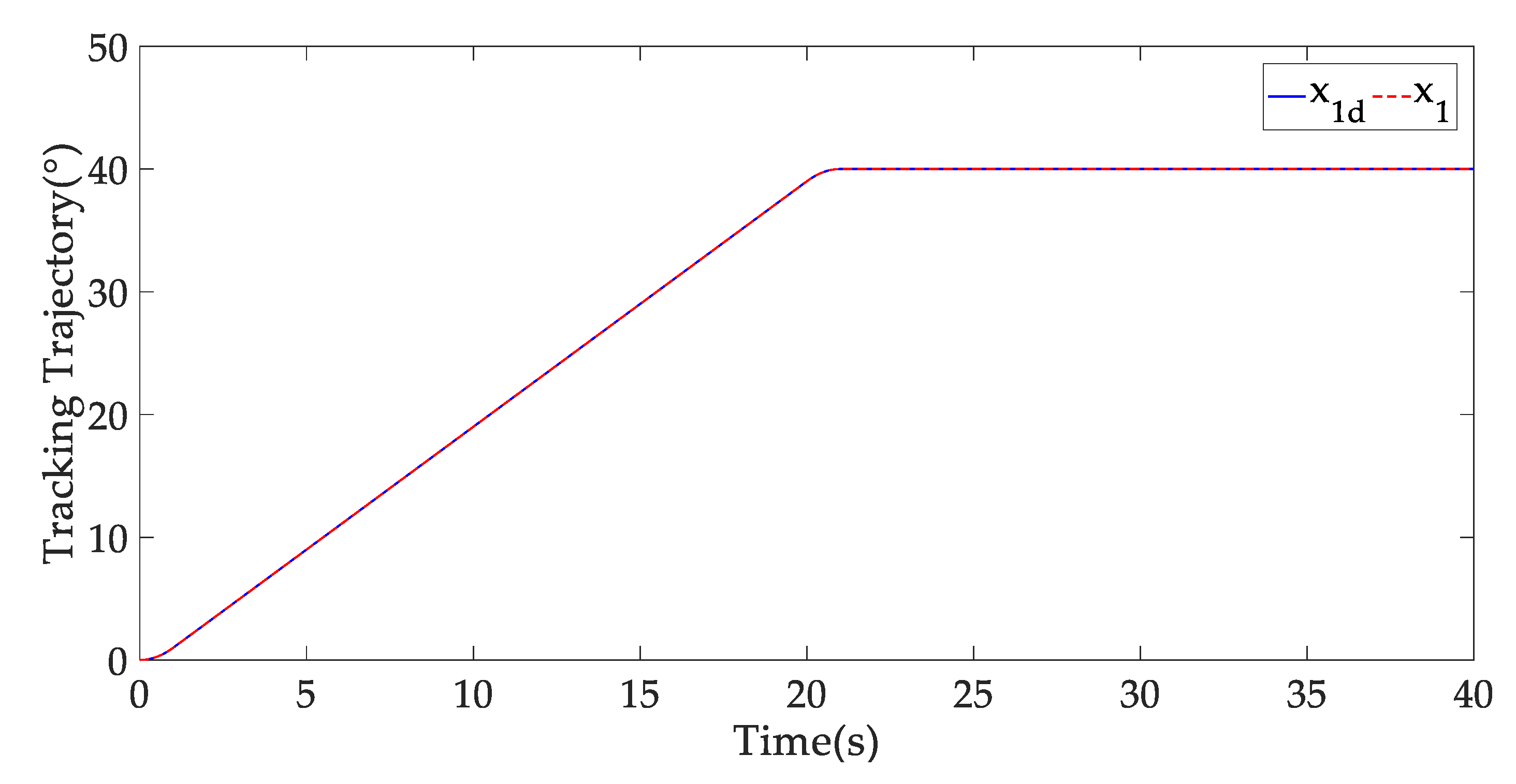
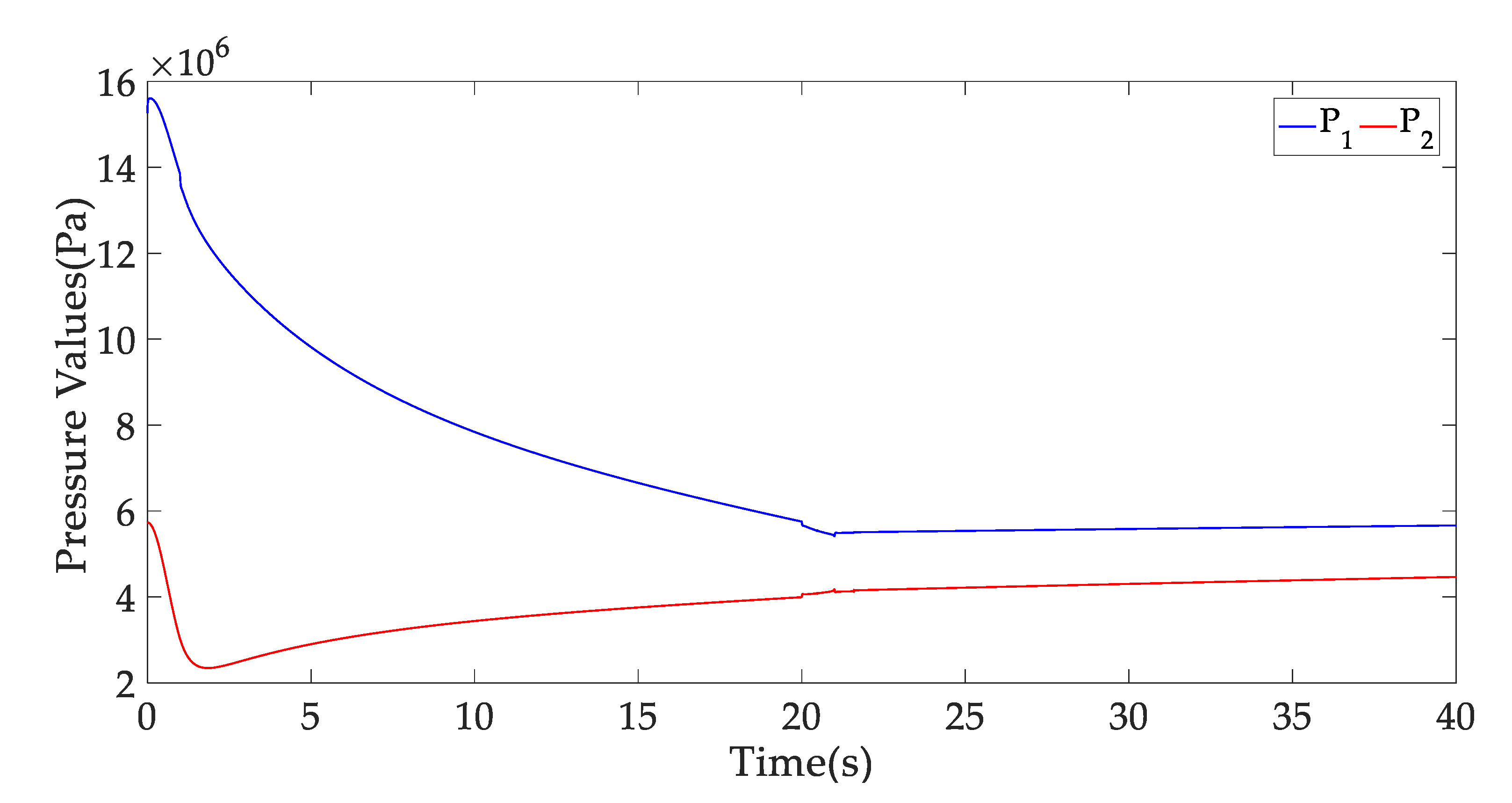
4. Simulation Results

The actual parameters of the electrohydraulic lifting mechanism of the launcher system can be observed from Table 1. The lifting mechanism is drove by the hydraulic cylinder. The function is defined as S f ( x 2 ) = 2 arctan ( 1000 x 2 ) / π The sample time is set as 0.5 ms.
Four controllers are compared to validate the effectiveness of the developed controller in the article.
(1) NRC: The nonlinear robust controller is proposed in Section 3, whose controller parameters are provided by k 1 = 100 , k 2 = 50 , k 2 s = 10 , k 3 = 50 , k 3 s = 30 , c 1 = 10 and c 2 = 30 . In addition, b 1 ( t ) = b 2 ( t ) = 1 t 2 + 500 .
(2) FLC: This is the feedback linearization controller introduced in [11], whose control law is
x 3 d = x s x 1 1 ( x 3 d a + x 3 d s ) x 3 d a = m g d 4 cos ( β 0 + x 1 ) + A f S f ( x 2 ) + B x 2 + J x ˙ 2 d ξ 1 , x 3 d s = k 2 ξ 2 u = ( u a + u s ) φ 1 , u a = φ 2 + x ˙ 3 d x s x 1 ξ 2 , u s = k 3 ξ 3
The deference between NRC and FLC is that the nonlinear feedback terms are not introduced into FLC. That is, k 2 s = 0 and k 3 s = 0 in FLC. The other control parameters are same as NRC.
(3) RC: This is the robust controller, whose control law is
x 3 d = x s x 1 1 ( J x ˙ 2 d k 2 ξ 2 ) u = ( x ˙ 3 d k 3 ξ 3 ) φ 1
The deference between FLC and RC is that the model-based compensation terms are not introduced into RC. The other control parameters are the same as FLC.
(4) PI: This is a proportional-integral controller that is widely applied in practice. The controller parameters are set as k p = 10 and k i = 10 , in which k p and k i stand for proportional gain and integral gain, respectively.
Case 1: First the reference tracking signal presented in Figure 3 is employed to test the control performance of the developed contr ol method. As seen from Figure 3, the reference tracking signal is a point–point tracking trajectory, whose velocity and acceleration values are at most 2°/s and 2°/s2, respectively. The tracking trajectory of NRC can be found in Figure 3. The corresponding control errors of the four controllers is collected in Figure 4. It is easy to observe that NRC proposed in this paper can attain the best control performance among the four controllers in terms of the transient and steady-state tracking performance. This is contributed to the model-based feedforward compensation and the nonlinear feedback terms introduced in NRC. Owing to the same model-based feedforward compensation technique, FLC can obtain the better control performance than RC. However, the control accuracy of FLC is worse when comparing with NRC, which indicates the validity of the nonlinear feedback terms in NRC. In addition, it can be seen the control performance of PI is superior to that of RC, which reveals that PI has the certain robust ability against uncertainties and disturbances by adopting proper feedback gains. However, for the lack of the model-based feedforward compensation method, PI can achieve the worse tracking performance when compared to NRC and FLC. That shows the effectiveness of the model-based feedforward compensation method. In the meanwhile, it can be deduced that the high feedback gains in NRC and FLC can be shunned via using the model-based feedforward compensation method. In addition, the control input of NRC is presented in Figure 5, which is regular. The pressure values of two chambers in NRC and cylinder force can be observed in Figure 6 and Figure 7.
Case 2: To further test the control performance of the developed control method, a fast reference tracking signal presented in Figure 8 is employed. As seen from Figure 8, the new reference tracking signal is a point–point tracking trajectory, whose velocity and acceleration values are at most 3°/s and 3°/s2, respectively. The tracking trajectory of NRC can be found in Figure 9. The corresponding control errors of the three controllers is collected in Figure 8, in which RC is omitted due to its low control accuracy. It is easy to observe that NRC proposed in this paper can attain the best control performance among the three controllers in terms of the transient and steady-state tracking performance. This is contributed to the model-based feedforward compensation and the nonlinear feedback terms introduced in NRC. In addition, the control accuracy of FLC is worse when comparing with NRC, which indicates the validity of the nonlinear feedback terms in NRC. However, similar to the case 1, for the lack of the model-based feedforward compensation method, PI can achieve the worse tracking performance when compared to NRC and FLC. That shows the effectiveness of the model-based feedforward compensation method. In addition, the control input of NRC is presented in Figure 10, which is regular and bounded. The pressure values of two chambers in NRC and cylinder force can be observed in Figure 11 and Figure 12. They are also bounded. Consequently, the merits of the presented control method are verified by Case 2 once again.

5. Conclusions

In this paper, the asymptotic tracking problem is investigated for electrohydraulic lifting mechanisms of launcher systems. To complete the work, the dynamic equations and state-space forms of the electrohydraulic lifting mechanism are firstly modeled. Based on the system model, a nonlinear robust controller is developed, in which a continuous nonlinear feedback term is used to remove the effects of uncertainties and disturbances on tracking performance. By applying the Lyapunov function, the asymptotic tracking stability of the closed-loop system is pledged. At the end, the simulation example of an actual electrohydraulic lifting mechanism of the launcher system is done to validate the effectiveness with the proposed controller. In addition, it is worth noting that the developed controller is designed based on the full-state feedback; however, only the position signal can be measured in most practical cases. Hence, as our future research, it is worth developing an output feedback based robust controller for electrohydraulic lifting mechanisms of launcher systems.

Author Contributions

Formal analysis, L.L. and X.Y.; Investigation, Y.J., X.Y. and J.Y.; Methodology, L.L. and Y.J.; Project administration, Y.J.; Writing—original draft, L.L. and Y.J. All authors have read and agreed to the published version of the manuscript.

Funding

This research was not supported by any funding.

Institutional Review Board Statement

Not applicable.

Informed Consent Statement

Not applicable.

Data Availability Statement

Data sharing not applicable.

Conflicts of Interest

The authors declare no conflict of interest.

References

  1. Lu, L.; Yao, B. Energy-Saving Adaptive Robust Control of a Hydraulic Manipulator Using Five Cartridge Valves with an Accumulator. IEEE Trans. Ind. Electron. 2014, 61, 7046–7054. [Google Scholar] [CrossRef]
  2. Lane, D.M.; Dunnigan, M.W.; Clegg, A.C.; Dauchez, P.; Cellier, L. A comparison between robust and adaptive hybrid position/force control schemes for hydraulic underwater manipulators. Trans. Inst. Meas. Control 1997, 19, 107–116. [Google Scholar] [CrossRef]
  3. Seron, J.; Martinez, J.L.; Mandow, A.; Reina, A.J.; Morales, J.; Garcia-Cerezo, A.J. Automation of the Arm-Aided Climbing Maneuver for Tracked Mobile Manipulators. IEEE Trans. Ind. Electron. 2013, 61, 3638–3647. [Google Scholar] [CrossRef]
  4. Koivumaki, J.; Mattila, J. Stability-Guaranteed Force-Sensorless Contact Force/Motion Control of Heavy-Duty Hydraulic Manipulators. IEEE Trans. Robot. 2015, 31, 918–935. [Google Scholar] [CrossRef]
  5. Li, L.; Lin, Z.; Jiang, Y.; Yu, C.; Yao, J. Valve deadzone/backlash compensation for lifting motion control of hydraulic manipulators. Machines 2021, 9, 57. [Google Scholar] [CrossRef]
  6. Yang, X.; Deng, W.; Yao, J. Neural network based output feedback control for DC motors with asymptotic stability. Mech. Syst. Signal Process. 2022, 164, 108288. [Google Scholar] [CrossRef]
  7. Sun, W.; Pan, H.; Gao, H. Filter-Based Adaptive Vibration Control for Active Vehicle Suspensions with Electrohydraulic Actuators. IEEE Trans. Veh. Technol. 2016, 65, 4619–4626. [Google Scholar] [CrossRef]
  8. Yang, X.; Yao, J.; Deng, W. Output feedback adaptive super-twisting sliding mode control of hydraulic systems with disturbance compensation. ISA Trans. 2021, 109, 175–185. [Google Scholar] [CrossRef] [PubMed]
  9. Huang, Y.; Pool, D.M.; Stroosma, O.; Chu, Q. Long-stroke hydraulic robot motion control with incremental nonlinear dynamic inversion. IEEE/ASME Trans. Mechatron. 2019, 24, 304–314. [Google Scholar] [CrossRef] [Green Version]
  10. Park, J.; Lee, B.; Kang, S.; Kim, P.Y.; Kim, H.J. Online Learning Control of Hydraulic Excavators Based on Echo-State Networks. IEEE Trans. Autom. Sci. Eng. 2017, 14, 249–259. [Google Scholar] [CrossRef]
  11. Kim, W.; Won, D.; Tomizuka, M. Flatness-Based Nonlinear Control for Position Tracking of Electrohydraulic Systems. IEEE/ASME Trans. Mechatron. 2014, 20, 197–206. [Google Scholar] [CrossRef]
  12. Choi, Y.-S.; Choi, H.H.; Jung, J.-W. Feedback Linearization Direct Torque Control with Reduced Torque and Flux Ripples for IPMSM Drives. IEEE Trans. Power Electron. 2016, 31, 3728–3737. [Google Scholar] [CrossRef]
  13. Yao, B.; Al-Majed, M.; Tomizuka, M. High-performance robust motion control of machine tools: An adaptive robust control approach and comparative experiments. IEEE/ASME Trans. Mechatron. 1997, 2, 63–76. [Google Scholar]
  14. Yao, B.; Bu, F.; Reedy, J.; Chiu, G.T.C. Adaptive robust motion control of single-rod hydraulic actuators: Theory and experiments. IEEE/ASME Trans. Mechatron. 2000, 5, 79–91. [Google Scholar]
  15. Mohanty, A.; Yao, B. Integrated direct/indirect adaptive robust control of hydraulic manipulators with valve deadband. IEEE/ASME Trans. Mechatron. 2011, 16, 707–715. [Google Scholar] [CrossRef]
  16. Yao, J.; Deng, W.; Jiao, Z. Adaptive control of hydraulic actuators with LuGre model-based friction compensation. IEEE Trans. Ind. Electron. 2015, 62, 6469–6477. [Google Scholar] [CrossRef]
  17. Yao, J.; Deng, W.; Sun, W. Precision Motion Control for Electro-Hydraulic Servo Systems with Noise Alleviation: A Desired Compensation Adaptive Approach. IEEE/ASME Trans. Mechatron. 2017, 22, 1859–1868. [Google Scholar] [CrossRef]
  18. Yang, X.; Deng, W.; Yao, J.; Liang, X. Asymptotic adaptive tracking control and application to mechatronic systems. J. Frankl. Inst. 2021, 358, 6057–6073. [Google Scholar] [CrossRef]
  19. Deng, W.; Yao, J.; Wang, Y.; Yang, X.; Chen, J. Output feedback backstepping control of hydraulic actuators with valve dynamics compensation. Mech. Syst. Signal Process. 2021, 158, 107769. [Google Scholar] [CrossRef]
  20. Xian, B.; Dawson, D.M.; de Queiroz, M.S.; Chen, J. A continuous asymptotic tracking control strategy for uncertain nonlinear systems. IEEE Trans. Automat. Contr. 2004, 49, 1206–1211. [Google Scholar] [CrossRef]
  21. Yao, J.; Deng, W.; Jiao, Z. RISE-Based Adaptive Control of Hydraulic Systems with Asymptotic Tracking. IEEE Trans. Autom. Sci. Eng. 2017, 14, 1524–1531. [Google Scholar] [CrossRef]
  22. Ge, Y.; Yang, X.; Deng, W.; Yao, J. Rise-based composite adaptive control of electro-hydrostatic actuator with asymptotic stability. Machines 2021, 9, 181. [Google Scholar] [CrossRef]
  23. Won, D.; Kim, W.; Tomizuka, M. High-gain-observer-based integral sliding mode control for position tracking of electrohydraulic servo systems. IEEE/ASME Trans. Mechatron. 2017, 22, 2695–2704. [Google Scholar] [CrossRef]
  24. Rath, J.J.; Defoort, M.; Karimi, H.R.; Veluvolu, K.C. Output Feedback Active Suspension Control With Higher Order Terminal Sliding Mode. IEEE Trans. Ind. Electron. 2017, 64, 1392–1403. [Google Scholar] [CrossRef]
  25. Yao, J.; Jiao, Z.; Ma, D. Extended-state-observer-based output feedback nonlinear robust control of hydraulic systems with backstepping. IEEE Trans. Ind. Electron. 2014, 61, 6285–6293. [Google Scholar] [CrossRef]
  26. Wang, S.; Tao, L.; Chen, Q.; Na, J.; Ren, X. USDE-Based Sliding Mode Control for Servo Mechanisms with Unknown System Dynamics. IEEE/ASME Trans. Mechatron. 2020, 25, 1056–1066. [Google Scholar] [CrossRef]
  27. Ba, D.X.; Dinh, T.Q.; Bae, J.; Ahn, K.K. An Effective Disturbance-Observer-Based Nonlinear Controller for a Pump-Controlled Hydraulic System. IEEE/ASME Trans. Mechatron. 2020, 25, 32–43. [Google Scholar] [CrossRef]
  28. Dong, Y.; Nuchkrua, T.; Shen, T. Asymptotical stability contouring control of dual-arm robot with holonomic constraints: Modified distributed control framework. IET Control Theory Appl. 2019, 13, 2877–2885. [Google Scholar] [CrossRef]
  29. Nuchkrua, T.; Leephakpreeda, T. Novel Compliant Control of Pneumatic Artificial Muscle Driven by Hydrogen Pressure under Varying Environment. IEEE Trans. Ind. Electron. 2021, 46, 1. [Google Scholar] [CrossRef]
  30. Deng, W.; Yao, J. Extended-State-Observer-Based Adaptive Control of Electrohydraulic Servomechanisms without Velocity Measurement. IEEE/ASME Trans. Mechatron. 2020, 25, 1151–1161. [Google Scholar] [CrossRef]
  31. Merritt, H. Hydraulic Control Systems; John Wiley & Sons: Hoboken, NJ, USA, 1967. [Google Scholar]
  32. Guo, Q.; Chen, Z. Neural adaptive control of single-rod electrohydraulic system with lumped uncertainty. Mech. Syst. Signal Process. 2021, 146, 106869. [Google Scholar] [CrossRef]
  33. Krstic, M.; Kanellakopoulos, I.; Kokotovic, P. Nonlinear and Adaptive Control Design; Wiley: New York, NY, USA, 1995. [Google Scholar]
Figure 1. The schematic diagram of the lifting mechanism.
Applsci 12 00893 g001
Figure 2. The control diagram of the lifting mechanism.
Applsci 12 00893 g002
Figure 3. The tracking trajectory of NRC.
Applsci 12 00893 g003
Figure 4. The tracking errors of four controllers.
Applsci 12 00893 g004
Figure 5. The control input in NRC.
Applsci 12 00893 g005
Figure 6. The pressure values of two chambers in NRC.
Applsci 12 00893 g006
Figure 7. The cylinder force in NRC.
Applsci 12 00893 g007
Figure 8. The tracking trajectory of NRC.
Applsci 12 00893 g008
Figure 9. The tracking errors of three controllers.
Applsci 12 00893 g009aApplsci 12 00893 g009b
Figure 10. The control input in NRC.
Applsci 12 00893 g010
Figure 11. The pressure values of two chambers in NRC.
Applsci 12 00893 g011
Figure 12. The cylinder force in NRC.
Applsci 12 00893 g012
Table 1. Physical parameters of the EHA system.
ParameterValueParameterValue
m (kg)10,000 B   ( N m s / rad )2.5 × 10⁵
J   ( kg m 2 )1.5 × 10⁵ A f   ( N m )3 × 10³
Ps (Pa)2.1 × 10⁶ k ( m 4 / ( s V N ) )7.937 × 10⁻⁸
Pr (Pa)0 β e (Pa)7 × 10⁸
A1 (m2)3.14 × 10⁻² C t   ( m 5 / ( s N ) )9.6 × 10⁻¹³
A2 (m2)1.6 × 10⁻²d1 (m)1.6
V01 (m3)3.1416 × 10⁻⁴d2 (m)2
V02 (m3)3.04 × 10⁻²d3 (m)3.5
g (m/s2)9.8d4 (m)3
θ 0 (rad)0.2648 β 0 (rad)0.2618
D (mm)200 d (mm)140
L c (mm)1900
Where D and d stand for the cylinder diameter and the piston rod diameter, respectively; L c stands for the cylinder stroke.
Publisher’s Note: MDPI stays neutral with regard to jurisdictional claims in published maps and institutional affiliations.

