
3D FEM Analysis of the Subsoil-Building Interaction

Department of Construction Materials Engineering and Geoengineering, Faculty of Civil Engineering and Architecture, Lublin University of Technology, 20-618 Lublin, Poland
Appl. Sci. 2022, 12(21), 10700; https://doi.org/10.3390/app122110700
Submission received: 6 July 2022
/
Revised: 20 September 2022
/
Accepted: 18 October 2022
/
Published: 22 October 2022
Abstract
:This paper presents the process of advanced numerical analysis of interaction between a building and the subsoil. The analysis covered a wide range of work for both computing and research. As part of the research work, field and laboratory subsoil tests were carried out, as well as geodetic measurements of building settlement and measurements of natural vibrations of an object. The computational work included the analysis of a total of 47 FEM models. The subsoil was described using the Modified Cam-Clay model, with parameters determined using field CPT and SDMT tests, as well as triaxial and edometric laboratory tests. Parts with geodetic benchmarks were separated from the building model, and then multi-variant calculations were made on smaller, partial models with parameters obtained from various methods. Calibration of the main models was performed using 8 partial models for which calculations were carried out in 4–5 variants of parameters. This gave a total of 38 partial models. Then, calculations were carried out on the full model of the building with subsoil. At each stage, the results of vertical displacements were compared to the geodetic values. The measured settlement of the real building in the time from the construction of the underground story to its use for the period of 1 year, was from 2.3 mm to 7.8 mm. The settlement from FEM calculations of small calibration models for the same benchmarks was from 2.0 mm to 9.8 mm with parameters derived from CPT tests and from 1.8 to 7.3 mm for parameters derived from SDMT. For the full building model, settlement from FEM calculations ranged from 2.2 to 8.8 for the variant with a simplified subsoil model, and from 3.7 to 10.5 for the model taking into account the inhomogeneity of the subsoil. As a result, it was found that the displacements from the numerical analysis were convergent with the geodetic values. Detailed numerical analyses also allowed to detect the deviations of the segments from the vertical and to indicate potential damage to the structure. It was also indicated how the work of the subsoil influences the stress distribution in selected structural elements. Behaviour of the subsoil has an impact on the behaviour of the building and its deformations, as well as on the distribution of stresses in the structural elements, and, as a result, on the change in the distribution of internal forces in the structure.
1. Introduction
Ground deformations have a major impact on the distribution of forces in a structure. In order to properly design a built structure, it is extremely important to reliably represent the behaviour of the subsoil underneath. Recent years have seen a very intensive development of analysis using the Finite Element Method (FEM). Due to the availability of more efficient machines, it is possible to make calculations for every larger model in much less time. Today’s design practically does not exist without using FEM, so it is important to share experiences and the results of such calculations in order to better calibrate models and obtain more reliable results. The interaction between built structures and the subsoil is often analysed as a two-dimensional issue, e.g., for a selected cross-section of the structure [1,2,3]. For axially symmetrical problems, a section of the structure can be used [4]. Three-dimensional models of buildings are the most reliable. However, many analyses are often limited to foundations and based on the assumption that there is a rigid subsoil underneath, or described with one-parameter stiffness [5,6,7]. Sometimes subsoil mass is modelled with a small fragment of the structure [8,9]. Three-dimensional analysis of a building with subsoil is a complicated and laborious issue, but it is the most reliable one [10,11,12]. Sometimes analyses are performed over a larger area, e.g., for a development concept [13] or a larger site stability analysis [14].
The present work describes the process of conducting a three-dimensional analysis of cooperation between a real building located in Lublin in eastern Poland and loess soil it is founded on. Research included studying the soil and the structure, numerical modelling and geodetic measurements. The final results are the product of subsequent iterations adapting model parameters to the actual behaviour of the objects. Figure 1 shows a graphical representation of the overall analysis.
The paper presents a broad analysis of the cooperation between the building and the subsoil. Such full-scale analyses are performed very rarely, as they require the collection of a large database (soil parameters, settlement measurements, control of subsequent construction phases), are labor-intensive and time-consuming (e.g., construction and calibration of FEM models, soil tests and geodetic measurements in a wide range). The implementation takes several years, because we need data obtained both before the start of construction (soil investigation), during the process (verification of dynamic response of construction), and during geodetic measurements carried out for several years after the completion (building settlement). Despite the time-consuming nature of the work, the results of such works are very valuable in the context of designing new buildings in similar ground conditions.
Loess is a specific type of soil, associated mainly with collapse settlement, but a proper analysis in the design process related to subsoil stiffness is extremely important. The available literature includes publications covering the analysis of foundation settlement on loess; however, these are works of a much smaller scope, including single foundations [15,16], or without FEM analyses covering entire buildings [17]. Additionally, apart from the author’s publication [18], there are no publications at all about FEM analysis in the loess of the Nałęczów Plateau. Despite a similar genesis (aeolian), soils may behave in different ways in different parts of the world.
To describe the behaviour of the subsoil, parameters that are derived in various types of subsoil studies are needed. Soil parameters determined by different methods can differ significantly [19,20,21]. One of the most important features of soil is its deformability, which shows a strong non-linearity and is variable depending on the range of deformations considered. The maximum soil stiffness is expressed by the initial shear modulus G0 and is associated with deformability in the range of very small deformations. As deformations increase, soil stiffness decreases with a non-linear relationship, as illustrated in the diagram by Atkinson [22,23]. This relationship, referred to as soil stiffness degradation curve (the so-called S curve), is presented in Figure 2 along with ranges of deformations for typical structures and the selection of appropriate research methods depending on the range of deformations. Studies on the deformability of Polish soils in a wide range of deformations have been described, inter alia, in [24,25,26,27,28]. Soil stiffness is the lowest in the limit state, i.e., at deformations of about ε = 0.1%.
In oedometric tests, compressibility is determined in the range of deformations that are close to shearing deformations. Oedometric modulus values are usually low. In reality, however, the soil most often interacts with the building—particularly in the case of stronger soils—in the range of much lower deformations. Therefore, adopting oedometric moduli in calculations of settlements for stronger soils often results in their significant overestimation. Weaker soils interact with structures within the range of larger deformations, i.e., in conditions similar to those from oedometric tests. Engineering practice and literature both confirm that actual settlements are much smaller than those estimated from the results of oedometric tests [25,29,30,31,32]. The most appropriate way to verify the adopted deformation parameters is to conduct geodetic measurements of building settlement.
2. Materials and Methods
2.1. Tests on a Real Building
The research concerned a large multi-family building with four floors above the ground and one underground, located in Lublin (Figure 3a). The entire building consists of three segments, separated from each other by movement joints at the foundations, arranged in the shape of the letter T. The horizontal dimensions are about 90 × 45 m. The object is located on a small slope, so each segment is lowered by half a floor in relation to the previous one. Segment A is the highest; the adjacent Segment B is lowered by half a floor, and Segment C is lowered by half a floor in relation to Segment B, and by one floor in relation to Segment A. The building has a mixed reinforced concrete and masonry structure. Walls are 25 cm thick, while reinforced concrete floors are 20, 22 and 30 cm thick. The building is founded on reinforced concrete footing and reinforced strip footing.
2.1.1. Subsoil Examination
Lublin is located in the area of the Nałęczów Plateau with loess covers (Figure 4). Basically, only in the valleys there are river formations from the ground level. In the uplands there are mainly loess soils, which are the basis for the foundations of buildings.
In order to determine soil characteristics, laboratory tests (among other, oedometric and triaxial compression tests) and field tests (CPT and SDMT) were performed, the location of which is shown in Figure 3b. A selected representative CPT chart is presented in Figure 5, and a detailed description of field tests can be found in [34].
During CPT tests, qc—tip resistance and fs—sleeve resistance are measured, which are the basis for determining other geotechnical parameters. The most important parameter for the purposes of the analysis was the constrained modulus MCPT, which was determined from the formula defined by Sanglerat [35]:
A slightly altered version of the formula is proposed by Senneset [36]
where qt—total cone tip resistance, σv0—vertical overburden stress.
Both in Sanglerat’s (Equation (1)) and Senneset’s (Equation (2)) formula, it is extremely important to select the empirical coefficient αm, which can assume a value in the wide range of 1 ÷ 15 [35,37,38]. Although the CPT test is performed in the presence of large deformations, by choosing a well-calibrated αm coefficient, the constrained modulus can be derived for any range of deformations, as in Figure 2. For loess from the vicinity of Łańcut, Młynarek and Wierzbicki [39,40] assumed the relationship Equation (2) with the coefficient αm = 8.25. For loess from Kazimierz Dolny, Frankowski [24] determined a much smaller coefficient αm = 2.5 for Equation (1). This coefficient was calibrated in relation to the constrained modulus from oedometric tests, i.e., in conditions of large deformations. Taking into account the above literature data and after the analyses conducted by the author of the present study [34], the relationship Equation (1) with the coefficient αm = 6 was adopted for loess soils. Further calculations confirmed that this is a correct value.
As far as SDMT tests are concerned, the most significant values for the purposes of the present analysis were the dilatometric constrained modulus MDMT, which was calculated using the Marchetti formula [41] and the lateral stress coefficient KD used to assess soil preconsolidation. These parameters are shown in Figure 6.
Loess soils from the vicinity of Lublin are normally consolidated (NC) due to their genesis. In order to confirm this, preconsolidation stress p0 from oedometric tests was analysed, as well as the distribution of KD coefficient with depth from SDMT tests. The results of oedometric tests confirm that the soil is normally consolidated, because the preconsolidation stresses from the study corresponded to the geostatic stress from the sampling depth.
The assessment of the degree of soil consolidation is expressed by the OCR indicator, which in DMT tests is not a directly measured parameter, but interpreted only on the basis of KD coefficient. The determination of the OCR indicator from DMT tests is related to the type of soil and local relationships. For cohesive soils, there are many regional interpretations, while for sandy soils, i.e., with ID > 1.2, determining OCR is much more difficult and according to the latest research, tip resistance qc from CPT probing is needed [42,43]. Loesses are transitional soils; therefore, determining OCR is not clear-cut, and the author was unable to find a credible interpretation determining OCR for these soils. Therefore, in order to present the nature of soil preconsolidation, the distribution of the KD coefficient with depth is shown in Figure 6, because notwithstanding the exact OCR value, the KD coefficient very well reflects the history of the soil. On the basis of Marchetti’s original formulas, it can be simplified that OCR = 1 for KD = 2. KD coefficients in Figure 6 indicate a slight preconsolidation of near-surface zones, which may be related to the temporary storage of soil from the neighbouring construction sites. It may also be the effect of “quasi-preconsolidation” associated with cementation of soil with calcium carbonate [39,42]. A significant increase of KD in the near-surface zone is a common phenomenon, often registered by the author in DMT tests on loess conducted in Lublin. In turn, deeper soil should be described as normally consolidated because KD~2. To sum up, the received KD charts show that the soil is normally consolidated, and the increase in OCR in the higher parts is typical for the near-surface zone [44,45], so it was assumed in the calculations that the soil is normally consolidated.
From three oedometric tests, the oedometric moduli Eoed = 4.4 ÷ 6.0 MPa for the stress range of 126 ÷ 252 MPa, and Eoed = 7.8 ÷ 10.1 MPa for the range of 252 ÷ 503 MPa were obtained. Unloading-reolading modulus assumed the value Eur = 48.5 ÷ 61.7 MPa. Effective internal friction angle φ’~35° and effective cohesion c’~5 kPa were obtained from TXCID triaxial tests. Selected laboratory tests results are presented in Figure 7. In addition, bulk density in the range of 1.75 ÷ 1.85 g/cm3, natural moisture wn = 8.3 ÷ 16.4% and porosity index e = 0.55 ÷ 0.76 were obtained in the basic tests.
Summing up, the subsoil in the area of the building is mainly composed of loess soils. Up to the depth of about 5 to 7 metres below the foundation level, there are loess silts of the aeolian facies, the so-called typical loess with a compact consistency and tip resistance qc = 4.6 ÷ 8.1 MPa (MCPT = 27.6 ÷ 48.6), with an average of 5.3 MPa, and the constrained modulus MDMT = 30 ÷ 60 MPa (locally up to 80 MPa) with an average of approximately 40 MPa. These are relatively high values. Below the loess, there is a thin sandy interbedding and, locally, slightly plasticised clay loess which is deposited on residual soil and cracked limestone. Taking into account the thickness of the loess cover, the type of foundation and magnitude of loads, loess soils have fundamental importance for and impact on the building. It was the parameters of these soils that were the focus in the recognition of the subsoil. In relation to the results obtained from tests conducted in the Lublin area [46,47,48], soil conditions should be considered typical and representative of the Lublin area, and loess subsoil in this area can be considered as a good load-bearing substrate. A representative geotechnical cross-sections are shown in Figure 8.
2.1.2. Building Settlement Measurements
In order to verify the calculations, a geodetic measurement network was established on the building, consisting of 18 points (10 outside the building, 5 inside the building and 3 reference benchmarks), followed by precise levelling measurements with an accuracy of 0.5 mm. During construction works, some benchmarks were destroyed, so only 8 points were left at the time of the last measurement (Figure 3b). In Table 1, the measuring stages are listed together with a description of the condition of the structure at the time of measurement and the loads assumed for the numerical model.
The displacement graph (Figure 9) indicates settlement stabilisation for most points. The largest displacement was recorded on benchmarks in the extreme parts of the building from the side of the slope (Z3, Z6, Z7), which may suggest a slight tilt of the building in this direction. For these points, the shape of the curves indicates that stabilisation of the building settlement has not occurred yet. The benchmark Z8 in the central part of the building is noteworthy, as according to measurements, it was elevated by about 1 mm. According to the author, this is probably related to the fact that the building is leaning towards the slope and to a kind of “break” at the point of expansion joints, and thus a possible rise of the building in the central part. Negligible elevation values recorded on nearby benchmarks Z1, Z5 and Z9 may confirm this hypothesis, but according to the author, they may just as well result from measurement errors and attest to settlement stabilisation.
2.1.3. Building Vibration Measurements
In the process of FEM modelling of the building, numerous simplifications are used that affect the reliability of the results of calculations. Vibration measurements were used to verify the correctness of the numerical model of the building. Tests were carried out on the structure that consisted of forcing vibrations on ceilings and measuring vertical accelerations. A total of 54 measurements were performed at various locations in the building, which allowed for identifying floor vibration frequencies. Verification of the correctness of the model of the building was described in [49].
2.2. Numerical Analyses of Real Buildings
2.2.1. Subsoil Model
After a review of the works [50,51,52,53,54], Modified Cam-Clay was chosen as the subsoil model. Its basic assumption is that for the primary load, there is a logarithmic relationship between the mean effective pressure p0 and the porosity index e (isotropic Normal Consolidation Line—NCL). NCL described as the compression index on the lnp’-e plane is a straight line with a slope of λ. The final stress level ever achieved on this line is called isotropic preconsolidation pressure ppo. [55,56,57]. During unloading and reloading up to preconsolidation stress, there is a line with slope of κ, referred to as unloading-reloading index. In reality, on the p’-e plane, there is an infinite number of recompression curves - secondary load curves, each of which corresponds to a specific ppo value [51,58]. Plane p’-e is shown in Figure 10a.
Yield surface, illustrated in Figure 10b, in the Modified Cam-Clay model is described by the ellipse equation, symmetrical in relation to the pc line:
where q is the stress deviator; M is the slope of the Critical State Line on the p-q surface (Figure 8b); pc is the isotropic stress equivalent to preconsolidation stress; and p is the average normal stress.
The M parameter is related to the effective angle of internal friction φ’ with the following relationship:
The extent of yield surface a0 in the Modified Cam-Clay model is described by the equation:
where e1 is the porosity index at the intersection of the NCL with the e axis on the lnp’-e plane; eo is the initial porosity index; and po is preconsolidation stress.
Summing up, the main parameters of the Modified Cam-Clay model necessary to model soil behaviour are λ, κ, M, a0, p0. These parameters can be determined directly in laboratory triaxial compression and oedometric tests. There are also approximate methods for estimating these parameters based on indirect research.
2.2.2. The Process of Building FEM Models and Their Assumptions
The calculations were carried out in the ABAQUS Standard (implicit solver) programme (version 6.14-2), licensed for the Lublin University of Technology in Poland, which uses the Finite Element Method (FEM). The analyses were carried out in stages on the model of the whole building, and on its sections, which is schematically presented in Figure 1. The construction of the model began with segment B. The model was created gradually, subsequently adding new elements (ceiling, wall, etc.) and performing modal analysis, which, after comparing the frequency of vibrations with measurements on the building, verified the correctness of the FEM model. Initially, the subsoil was excluded from the model, and the building was supported by rigid supports instead of foundations. Then, calculations were carried out on small calibration models of a section of the structure with the subsoil mass underneath. In the final stage, calculations were made for the entire building, including the subsoil mass. Ultimately, 47 numerical models were built and analysed, of varying degrees of complexity, from small ones simulating the behaviour of a subsoil sample, to full “building-subsoil” models.
2.2.3. FEM Numerical Model of the Building
The FEM numerical model of the building was created as a shell model with beam elements of linear elastic behaviour. Walls, ceilings and binding joists were built of four-node S4R shell elements. The columns were constructed as beam elements (cf. [7]). The foundations constituting the transition between the building (linear elastic, shell-beam model) and the subsoil (elastic-plastic solid model) were modelled with C3D8R solid elements. Wall elements were adopted in the axes of structural elements, while the ceilings were located in their upper plane and the appropriate eccentricity was introduced. Reinforced concrete elements were assigned the following properties: bulk density ρ = 2.5 t/m3, Poisson’s ratio ν = 0.2 [59] and Young’s modulus E = 34.9 GPa, which was estimated based on the degree of reinforcement of the cross-section [49]. For masonry parts, the following were adopted: ρ = 1.7 t m3, ν = 0.25 and E = 4.5 GPa, determined in accordance with PN-EN 1996-1-1 norm [60].
Due to the mixed technology of reinforced concrete and masonry, the problem arose of how to model the “wall-ceiling-wall” connection, described, among others, in [7]. Therefore, different variants of connections between reinforced concrete-masonry elements were analysed, which was described in detail in [49]. It was determined that the connections are characterised by an indirect nature of interactions, though they are closer to a rigid connection. Further calculations assumed rigid connections for all elements.
2.2.4. FEM Numerical Model of the Subsoil
The FEM numerical model of the subsoil was created as a solid model from 20-node C3D20R elements. The output parameters of the Modified Cam-Clay model were determined from oedometric and triaxial tests. The deformation parameters λ and κ were calculated from the e-ln(σ) charts (Figure 11), based on the slope of the lines in particular stress ranges.
Basing on oedometric and SDMT tests, it was assumed that the soil is NC and the stress p0 corresponds to geostatic stress. The M parameter of the Modified Cam-Clay model was calculated from Equation (4), assuming φ′ = 35°. The range of the yield surface a0 was determined on the basis of porosity indices e0 and e1 from laboratory tests and consolidation charts. Finally, the results from the three samples were compiled in Table 2, and these were the output parameters for calculations.
The construction process of the subsoil model was divided into two main parts: a large model of the subsoil under the building and a number of smaller calibration sub-models, on which calculations were made with different variants of subsoil parameters. Eight small models were built to map a fragment of the building structure where measurement benchmarks were placed, which is schematically shown in Figure 12.
2.2.5. Calibration of the Subsoil Numerical Model—Partial Models
Calibration of subsoil parameters was performed on partial models. In order to standardise the calculations, subsoil mass with a depth of 12.0 m below the foundation level and dimensions in the plan view of 6.0 × 6.0 m was adopted, in accordance with Fedorowicz’s guidelines [61], which were developed on the basis of several dozen literature items by various authors. Each submodel consisted of three parts: a wall section with a benchmark, foundation and subsoil mass. For the subsoil and structure, solid elements were adopted (C3D8R—for the structure and C3D20R—for the subsoil). The dimensions of the finite element mesh were about 0.1 m for the wall and foundation and about 0.2 m for the subsoil at the connection point with the foundation. With the increase in distance from the foundation, the dimensions of the subsoil mesh increased, reaching in the farthest areas a side length of about 1.5 m. Standard geotechnical boundary conditions were used to block horizontal movement perpendicular to the plane on the sides and vertical movement at the base of the subsoil mass. Ultimately, the models consisted of 1892 ÷ 8940 solid elements and 7039 ÷ 32,583 nodes, with a total number of degrees of freedom in the range of 21,117 ÷ 97,749. No calculations were made for benchmarks Z2 and Z10 because they had been destroyed.
A linear elastic model was used for the structure, and parameters of C25/30 concrete were assigned to it. The subsoil was modelled in 5 parameter variants (Table 3). The internal friction angle, bulk density and secondary compressibility, i.e., the parameters of the Modified Cam-Clay M and κ model, were assumed to be invariant, respectively φ′ = 35°, ρ = 1.8 g/cm3, Eur = 55.1 MPa. Primary compressibility for variants with parameters from in situ tests was taken by probing closest to the studied benchmark in accordance with the areas in Figure 3b.
The initial variant was EDO1, where all parameters were derived on the basis of laboratory tests. In the EDO2 variant, the results were modified assuming that stabilisation of settlements in oedometric tests occurred after two hours. This increased the constrained moduli. In the CPT1 variant, the initial compressibility was derived from CPT static sounding. Because Modified Cam-Clay parameters are not directly obtained in CPT probing, the author developed an original conversion procedure. Due to OCR~1 and foundation at a depth of approximately 4 ÷ 7 m, it was assumed that for stresses of about 70 ÷ 120 kPa, the subsoil behaviour is in the range of secondary stresses, and the parameter κ was adopted from oedometric tests, i.e., κ = 0.0014. Additional stresses range from 70 to 250 kPa. Therefore, in order to determine the λ parameter, the actual results of oedometric tests for the stress range of 126 ÷ 252 kPa were “modified,” assuming that the constrained modulus from CPT soundings occurs in this range. Subsequently, the compressibility index Cc was calculated, and the LPO slope was determined from the relationship λ = Cc/2.3.
In the CPT1 variant, homogeneous subsoil was assumed, and parameters of the layer directly below the foundation were adopted for the entire depth. In the CPT2 variant, the parameters were derived in a similar way; however, layered subsoil was assumed, in accordance with the divisions based on CPT, as in Figure 5. Division into sublayers was performed only for the zone directly below the foundation. Changes below 6 m from the bottom of the foundation were not taken into account due to their negligible impact on settlement. In the DMT variant, the parameters were derived from SDMT tests using a transitional procedure like in CPT probing. For area E, where for technical reasons the SDMT test could not be performed, calculations in variant 5 were not carried out. Finally, the parameters listed in Table 4 were adopted in calculations.
The analysis was divided into computational steps in which the phases of constructing the building were subsequently mapped, as described in Table 1 In the first step, Geostatic, the state of stress was introduced into the subsoil. In the second step, Footing, the geometry of the foundation and wall section were introduced. Then, in the next four steps, Load 0 ÷ 3, the load was increased in accordance with its values measured during the subsequent geodetic surveys. The load was applied in the form of an even pressure in the upper plane of the wall, calculated proportionally from the stresses in the area at the contact point between the foundation and the subsoil from the numerical model of the whole object. The procedure of calibrating partial models is described in detail in [62]. The results of the calculations were displacements and stresses in particular construction phases. The shape of the isolines in maps of stresses and displacements differed slightly for various parameter variants. In turn, the values of vertical displacements were significant. Selected bitmaps for the Z1 model are shown in Figure 13.
The calculation results for all models and parameter variants are compiled in Table 5. The values of displacement were given in relation to the Load 0 step, so that they could be compared with geodetic measurements. Differences between calculated and measured values were also given. Positive values (green) mean that the calculated settlement was larger than the actual settlement, while negative values (red) mean that calculated settlement was smaller than the actual settlement. The largest displacements were obtained in calculation variants with parameters determined from oedometric tests (EDO1 and EDO2). These values were always much higher and significantly exceeded actual settlements. Settlements calculated on parameters from in situ soundings gave values much more similar to actual settlements. In the case of CPT soundings, the forecasted settlement is rather higher than the actual settlement, while for SDMT tests it is slightly lower. The relative error of estimation δ was also determined in relation to the allowable settlements of 50 mm, in accordance with Eurocode 7 [63].
For the EDO1 variant, the relative error was in the range of 10÷78%, with a mean of 49%, while for EDO2—in the range of 3÷71%, with a mean of 29%. Estimation errors for these variants should be considered large. For variants with CPT parameters, the error ranged from 1 to 18%, with a mean of 8% for simplified homogeneous subsoil (CPT1) and 7% for layered subsoil (CPT2). The values rather indicate a tendency to overestimate settlements (which is a safer assumption), and this result can be considered very good. For the DMT variant, the error ranged from 1 to 7%, with a mean of 3%. The fit value is the best possible; however, the estimated settlements were usually smaller than the actual ones. This result should also be considered very good.
The chart presenting benchmark displacement over time (Figure 9) indicates that building settlement is stabilising; only some benchmarks, those located on the edge of the building at the slope (Z3, Z6, Z7) show that settlement of the structure is going to continue for some time. Therefore, settlements larger than those measured from CPT variants may be even closer to the actual ones after some time. Taking into account small actual settlements in relation to the allowable values and the complexity of the structure, the author found the fit of the results very good.
2.2.6. Numerical Analysis of the Full “Building-Subsoil” Model
After calibration on small models, two variants of parameters were adopted for the subsoil in the full model (Table 6). In the first variant, HOMO, constant parameters were adopted for the entire subsoil. In the second variant, AREA, the subsoil was divided into computational areas (Figure 14) and soil parameters were assigned to them in accordance with in situ tests from these areas. For homogeneous subsoil, the mean of the parameters for particular areas was adopted. Moreover, calculations were performed in the RIGID variant for the model of the building without subsoil—with rigid supports. The meshing for the full model started from the building. A mesh with sides of approximately 0.2 m was adopted, starting its creation from the smallest elements of the building. In the subsoil, in the zone of contact with the building, a mesh of similar dimensions, about 0.2 m, was used. Along with the depth and distance from the building, the dimensions of the mesh were increased. In the deepest parts of the subsoil, a mesh with dimensions of up to 3.6 m was used. Standard geotechnical boundary conditions were used to block horizontal movement perpendicular to the plane on the sides and vertical movement at the base of the subsoil mass. The full “building-subsoil” model was made up of 218,532 finite elements: solid, plate and beam elements with the dimensions of the subsoil element ranging from 0.2 to 3.6 [61]. In total, the model consisted of 502,224 nodes with 1,921,455 degrees of freedom.
3. Results
In the analysis, subsequent fragments of the building were gradually applied to the model, in accordance with the actual construction stages. The calculations were divided into 13 steps similar to the calibration models, starting from Geostatic and Footing. Then, in 9 steps: Underground (a ÷ c), Load 0 (a ÷ c) and Load 1 (a ÷ c), the geometry of the building was introduced. In the last two steps, Load 2 and Load 3, additional load was added for phase 2 and 3 respectively from Table 1. Figure 15 shows the displacements of the model in the AREA variant in selected calculation steps. Figure 16 shows the vertical displacements of the RIGID and AREA models.
Table 7 lists the actual and calculated vertical displacements, as well as absolute and relative calculation errors. The average settlement and calculation error for the HOMO and AREA models were almost the same. However, there are local discrepancies in the results, which proves that the heterogeneity of the loess subsoil causes non-uniform settlement of the building. Benchmark displacements in the RIGID model were only the effect of the compressibility of the construction material and were ultimately below 1 mm. The difference of displacements calculated for particular phases was about 0.1 ÷ 0.2 mm.
Figure 17 shows the map of displacements in a cross-section through the building. The settlement change with depth for the places where benchmarks were installed is shown in Figure 18 These are total displacements from the beginning of construction. In models with the subsoil, HOMO and AREA, it was observed that the C segment tilts from the B segment. The displacements in cross-sections with expansion joints between these segments for the HOMO and RIGID models are shown in Figure 19. In reality, this phenomenon also took place because benchmarks located on the edge of segment C (Z6, Z7) show greater settlement than benchmarks located in the central part of the building (Z4, Z5, Z8). In the RIGID model, naturally, no tilting of the building was observed.
The total displacements for HOMO and AREA models are compared in Figure 20. The areas with differences are marked in the figure. In reality, in these areas, when the boundary stress for the construction material is exceeded, scratches may appear on the walls of the building.
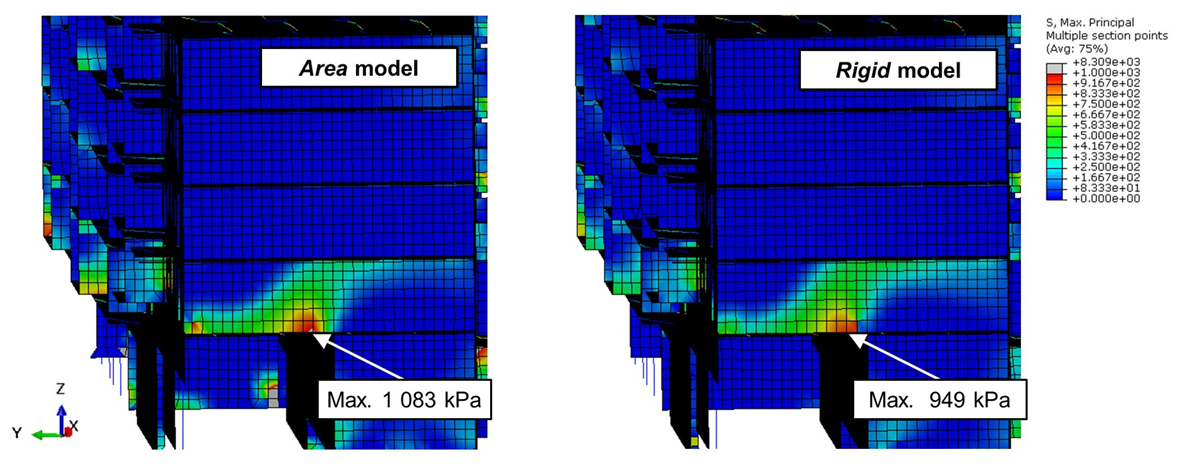
Uneven settlement of the building affects the distribution of stress in structural elements. The maps of minimum principal stress for the AREA and RIGID models are compared in Figure 21. There are noticeable differences in stress distribution. This particularly applies to structural elements in the lowest part of the building. On the top floors, the differences are negligible. Figure 22 shows a close-up of the wall at the garage entrance, where there are evident differences in stress distribution. In the RIGID model, stresses are distributed more evenly, while in the AREA model, there is a stress concentration in the column strips in the wall. The differences can be substantial, and the values in the lowest nodes differ more than three times.
Figure 23 shows the maximum principal stress distribution for the selected reinforced concrete deep beam, where there were also differences in the results for models with the subsoil and with rigid supports. They concerned both the shape of stress isolines and values. For the presented reinforced concrete deep beam it was approximately 14%. In other reinforced concrete deep beams, the differences reached up to 20%.
4. Discussion
The identified differences between the model with or without subsoil attest to the significant impact of the subsoil on deformations and stress distribution in the structure and prove the need to take this effect into account in design calculations. The demonstrated results are an excerpt of the most important results and are presented in order to indicate the occurring differences. As a result of the conducted work, it was determined that for loess, the use of direct oedometric test results in numerical calculations results in obtaining settlements much larger than in reality. Oedometric constrained moduli reached Eeod < 10 MPa, which is consistent with the results of other researchers [24,29,64,65,66,67,68,69]. However, settlements calculated using FEM with these parameters significantly exceed the values measured in reality. The results coincident with the actual displacements were obtained with the parameters from CPT and SDMT tests. Constrained moduli from in situ tests are at a similar level in the range of 30 ÷ 60 MPa; therefore, settlements estimated using them give similar results. The values of oedometric moduli are the lowest, while MDMT are slightly higher (by about 10%) than MCPT, which is in line with the adopted assumptions of the trend of the stiffness degradation curve (Figure 2).
The values of settlement determined in the numerical analyses differ slightly from the measured values. No direct parameters of the Modified Cam-Clay model are obtained from CPT and SDMT field tests. These parameters were derived in the process of transformation of the results. According to the author, despite the use of a greater number of simplifications and transformations in relation to direct oedometric tests, this procedure is appropriate, as it enables obtaining values of settlements more similar to actual ones.
The author conducted a similar analysis for a tall building in Lublin situated on a foundation slab. With similar calculation assumptions, the obtained calculation results were consistent with the real building settlement measurements [18]. The analysis is difficult to compare with the results of other researchers, because for the loess of the Nałęczów Plateau, such a detailed FEM analysis of the cooperation of the subsoil with the building was not performed. On the other hand, referring to the results of analysis for loess in other regions of the world, Milovic and Djogo [17] analysed the settlement of buildings erected on loess in Belgrade (Serbia). Those buildings settled much more, from a few to even more than 40 cm. However, they were loess with different parameters, much lower qc in the range of 1.0–3.0 MPa and with a weight from 12.6 to 17.2 kN/m3, so much lower than the analysed ones. Santrač et al. [70] conducted analyses of the settlement of a silo located in the loess near the village of Novi Sad in Serbia. They also obtained a settlement of more than 20 cm. However, also in this case, they were loess with a much lower weight of 12.6–14.1 kN/m3 and qc in the range of 1.9–3.5 MPa. Large loess covers lie in China. Analyses including FEM calculations for the improved loess subsoil were presented in [71]. The subsoil was improved due to the collapsing nature of loess. The soil was also characterized by a low weight, approximately 15.1 kN/m3. In all these examples the loess was characterized by a relatively low density, which is due to the macroporosity. The analysed loess in Lublin, in the foundation zone and below had a weight of 18.1 kN/m3 and a qc in the range of 5.0–8.0 MPa. Thus, they were characterized by much higher parameters. According to the author, significant settlement should be associated mainly with macropores, i.e., low soil density.
The analysed loess, despite a similar origin, are characterized by much more favourable geotechnical parameters compared to those deposits from other parts of the world. One of the reasons for taking up the topic, despite a similar origin, was the strong differentiation of subsoil behaviour. There is a need for regional data collection as loess from different regions of the world may have different behaviour.
On the other hand, this diversity requires careful implementation of the results for land in other regions of the world and their limited use. The performed analysis may be a comparable experience according to Eurocode 7 for buildings founded on loess in the Lublin region with similar dimensions and loads. Constructions, e.g., tall buildings, whose range of cooperation with the ground is greater or diaphragm walls may differ from the results for the analysis in question. It may also constitute a reference level for buildings founded on loess in other regions of the world, provided that the parameters of in situ tests are similar.
5. Conclusions
Behaviour of the subsoil has an impact on the behaviour of the building and its deformations, as well as on the distribution of stresses in the structural elements, and, as a result, on the change in the distribution of internal forces in the structure. The use of rigid fastening which models the foundation may lead to omitting significant problems in the behaviour of the building which occur during its use, such as uneven settlement. In the case of extensive buildings, there are usually areas of the subsoil with distinct parameters and this aspect should also be taken into account in static-strength analyses.
Currently, the author is conducting research on the characteristics of loess stiffness in the full range of strain. The development of reliable stiffness degradation curves will allow for the implementation of more advanced soil constitutive models, such as Hardening Soil Small (HSS), taking into account the work in the field of small strain.
Funding
This research received no external funding.
Institutional Review Board Statement
Not applicable.
Informed Consent Statement
Not applicable.
Data Availability Statement
Not applicable.
Conflicts of Interest
The authors declare no conflict of interest.
References
- Chai, J.; Shen, S.; Ding, W.; Zhu, H.; Carter, J. Numerical investigation of the failure of a building in Shanghai, China. Comput. Geotech. 2014, 55, 482–493. [Google Scholar] [CrossRef]
- Grodecki, M. Numerical Modelling of a Sheet Pile and Diaphragm Walls. Ph.D. Thesis, Cracow University of Technology, Kraków, Poland, 2007. (In Polish). [Google Scholar]
- Lechowicz, Z.; Kiziewicz, D.; Wrzesiński, G. Bearing capacity assessment of subsoil in undrained conditions under pad foundation subjected to inclined load according to Eurocode 7. Acta Archit 2013, 12, 51–60. (In Polish) [Google Scholar]
- Biały, M. Application of FC + MCC model in numerical analysis of cooling tower with subsoil. Czas. Tech. 2008, 3-Ś, 21–29. (In Polish) [Google Scholar]
- Kowalska, A. Analysis of the Influence of Non-Structural Elements on the Dynamic Characteristics of Buildings. Ph.D. Thesis, Cracow University of Technology, Kraków, Poland, 2007. (In Polish). [Google Scholar]
- Mrozek, D.; Mrozek, M.; Fedorowicz, J. The protection of masonry buildings in a mining area. Procedia Eng. 2017, 193, 184–191. [Google Scholar] [CrossRef]
- Mrozek, D. Nonlinear Numerical Analysis of the Dynamic Response of Damaged Buildings. Ph.D. Thesis, The Silesian Technical University in Gliwice, Gliwice, Poland, 2010. (In Polish). [Google Scholar]
- Przewlocki, J.; Zielinska, M. Analysis of the behavior of foundations of historical buildings. Procedia Eng. 2016, 161, 362–367. [Google Scholar] [CrossRef] [Green Version]
- Nepelski, K. The verification of subsoil parameters based on back analysis of a bridge. Bud. i Archit. 2014, 13, 39–48. (In Polish) [Google Scholar] [CrossRef]
- Comodromos, E.M.; Papadopoulou, M.C.; Konstantinidis, G.K. Effects from diaphragm wall installation to surrounding soil and adjacent buildings. Comput. Geotech. 2013, 53, 106–121. [Google Scholar] [CrossRef]
- Ko, J.; Cho, J.; Jeong, S. Nonlinear 3D interactive analysis of superstructure and piled raft foundation. Eng. Struct. 2017, 143, 204–218. [Google Scholar] [CrossRef]
- Słowik, L. The Influence of the Slope of the Land Caused by Underground Mining on the Inclination of Buildings. Ph.D. Thesis, Instytut Techniki Budowlanej, Warsaw, Poland, 2015. (In Polish). [Google Scholar]
- Michalak, H.; Przybysz, P. The Use of 3D Numerical Modeling in Conceptual Design: A Case Study. Energies 2021, 14, 5003. [Google Scholar] [CrossRef]
- Bovolenta, R.; Bianchi, D. Geotechnical Analysis and 3D Fem Modeling of Ville San Pietro (Italy). Geosciences 2020, 10, 473. [Google Scholar] [CrossRef]
- Labudkova, J.; Cajka, R. Experimental Measurements of Subsoil–Structure Interaction and 3D Numerical Models. Perspect. Sci. 2016, 7, 240–246. [Google Scholar] [CrossRef] [Green Version]
- Labudkova, J.; Cajka, R. 3D Numerical Model in Nonlinear Analysis of the Interaction between Subsoil and Sfcr Slab. Int. J. GEOMATE 2017, 13, 120–127. [Google Scholar] [CrossRef]
- Milovic, D.; Djogo, M. Differential Settlement of Foundations on Loess. In Proceedings of the International Conference on Case Histories in Geotechnical Engineering, Chicago, IL, USA, 2 May 2013; pp. 1–10. [Google Scholar]
- Nepelski, K. A FEM Analysis of the Settlement of a Tall Building Situated on Loess Subsoil. Open Eng. 2020, 10, 519–526. [Google Scholar] [CrossRef]
- Godlewski, T.; Kotlicki, W.; Wysokiński, L. Geotechnical Design According Eurocode 7; Wyd. ITB: Warsaw, Poland, 2011. (In Polish) [Google Scholar]
- Wszędyrówny-Nast, M. Estimation of the modulus of elasticity determination methods for the displacements analysis of the diaphragm wall. Geologos 2007, 11, 303–310. (In Polish) [Google Scholar]
- Młynarek, Z. Site investigation and mapping in urban area. In Proceedings of the XIV European Conference on Soil Mechanics and Geotechnical Engineering, Madrid, Spain, 24–27 September 2007; Volume 1. [Google Scholar]
- Atkinson, J.; Sallfors, G. Experimental determination of soil properties. In Proceedings of the 10th ECSMFE, Florence, Italy, 26–30 May 1991. [Google Scholar]
- Mair, R. Developments in geotechnical engineering research: Application to tunnels and deep excavations. Proc. Inst. Civ. Eng. Civ. Eng. 1993, 93, 27–41. [Google Scholar]
- Frankowski, Z.; Pietrzykowski, P. Displacement parameters of loesslike soils from southeastern Poland. Przegląd Geol. 2017, 65, 832–839. (In Polish) [Google Scholar]
- Truty, A. Small strain stiffness of soils. Numerical modeling aspects. Czas. Tech. 2008, 3, 107–126. (In Polish) [Google Scholar]
- Superczyńska, M. Values of elasticity parameters in the field of small and medium deformation range for Warsaw clays of the Poznań Formation. Inżynieria Morska i Geotech. 2015, 3, 207–211. (In Polish) [Google Scholar]
- Sas, W.; Gabrys, K.; Szymański, A. Analysis of stiffness of cohesive soils with use of resonant column. Inżynieria Morska Geotech. 2012, 4, 370–376. (In Polish) [Google Scholar]
- Lipiński, M. Criteria for Determining Geotechnical Parameters; SGGW: Warsaw, Poland, 2013. (In Polish) [Google Scholar]
- Borowczyk, M.; Frankowski, Z. Variability in geotechnic properties of loesses in the light of modern studies. Kwart. Geol. 1977, 23, 447–461. (In Polish) [Google Scholar]
- Szulborski, K.; Wysokiński, L. Assessment of the interaction of the structure with the subsoil in the diagnosis of building damage. In Proceedings of the VIII Conference Construction Appraisal Problems, Cedzyna, Poland, 2004. (In Polish). [Google Scholar]
- Godlewski, T.; Szczepański, T. Non-linear soil stiffness characteristic (Go)—Methods of determination, examples of application. Górnictwo i Geoinżynieria 2011, 2, 243–250. (In Polish) [Google Scholar]
- Gryczmański, M. An attempt of classification of constitutive models for soils. Zesz Nauk Politech Śląskiej 1995, 81, 433–446. (In Polish) [Google Scholar]
- Available online: www.asa-architekci.eu (accessed on 10 February 2018).
- Nepelski, K. Interpretation of CPT and SDMT tests for Lublin loess soils exemplified by Cyprysowa research site. Bud. I Archit. 2019, 18, 63–72. [Google Scholar] [CrossRef] [Green Version]
- Sanglerat, G. The Penetrometer and Soil Exploration; Elsevier: Amsterdam, The Netherlands, 1972. [Google Scholar]
- Senneset, K.; Janbu, N.; Svano, G. Strenght and deformation parameters from cone penetration tests. In Proceedings of the 2nd European Symposium on Penetration Testing, Amsterdam, The Netherlands, 1982. [Google Scholar]
- Ciloglu, F.; Cetin, K.O.; Erol, A.O. CPT-based compressibility assessment of soils. In Proceedings of the International Symposium on Cone Penetration Testing, Las Vegas, USA, 2014; pp. 629–636. [Google Scholar]
- Kulhawy, F.H.; Mayne, P.H. Manual on Estimating Soil Properties for Foundation Design; Electric Power Research Institute: New York, NY, USA, 1990. [Google Scholar]
- Młynarek, Z.; Wierzbicki, J.; Mańka, M. Geotechnical parameters of loess soils from CPTU and SDMT. In Proceedings of the International Conference on the Flat Dilatometer DMT, Roma, Italy, 2015; pp. 481–489. [Google Scholar]
- Młynarek, Z.; Wierzbicki, J.; Mańka, M. Constrained deformation and shear moduli of loesses from CPTU and SDMT tests. Inżynieria Morska i Geotech. 2015, 36, 193–199. (In Polish) [Google Scholar]
- Marchetti, S. In situ tests by flat dilatometer. J. Geotech. Eng. Div. 1980, 105, 299–321. [Google Scholar] [CrossRef]
- Marchetti, S. Some 2015 Updates to the TC16 DMT Report 2001. In Proceedings of the 3rd International Conference on the Flat Dilatometer, Rome, Italy, 2015; pp. 43–65. [Google Scholar]
- Lechowicz, Z.; Szymański, A. Deformation and Stability of Embankments on Organic Soils Part I. Research Methodology; SGGW: Warsaw, Poland, 2002. (In Polish) [Google Scholar]
- Jamiolkowski, M.; Ladd, C.C.; Germaine, J.T.; Lancellotta, R. New developments in field and laboratory testing of soils. In Proceedings of the 11th International Conference on Soil Mechanics and Foundation Engineering, San Francisco, CA, USA, 1985; pp. 57–154. [Google Scholar]
- Fedorowicz, L.; Fedorowicz, J. Preservation of pre-consolidated soils loaded with construction—Numerical modeling. Geoinżynieria Drog Most Tunele 2010, 25, 22–27. (In Polish) [Google Scholar]
- Nepelski, K.; Rudko, M. Identification of geotechnical parameters of Lublin loess subsoil based on CPT tests. Przegląd Nauk. Inżynieria I Kształtowanie Sr. 2018, 27, 186–198. (In Polish) [Google Scholar] [CrossRef]
- Nepelski, K.; Lal, A. CPT parameters of loess subsoil in Lublin area. Appl. Sci. 2021, 11, 6020. [Google Scholar] [CrossRef]
- Nepelski, K. Characteristics of the Lublin loess as a building subsoil. Prz. Geol. 2021, 69, 835–849. (In Polish) [Google Scholar] [CrossRef]
- Nepelski, K.; Błazik-Borowa, E.; Lipecki, T.; Bęc, J. Verification of the building FEM model on the basis of natural vibrations measurements. In Proceedings of the 3rd Polish Congress on Mechanics and 21st International Conference on Computer Methods in Mechanics, Gdańsk, Poland, 2015; Volume 1. [Google Scholar]
- Miller, H.; Djerbib, Y.; Jefferson, I.; Smalley, I. Collapse Behaviour of Loess Soils; ISRM Int. Symp., International Society for Rock Mechanics and Rock Engineering: Melbourne, VIC, Australia, 2000. [Google Scholar]
- Abed, A. Numerical Modeling of Expansive Soil Behavior. Ph.D. Thesis, Universität Stuttgart, Stuttgart, Germany, 2008. [Google Scholar]
- Helwany, S. Applied Soil Mechanics with ABAQUS Applications; John Wiley & Sons Ltd.: Hoboken, NJ, USA, 2007. [Google Scholar]
- Deng, G.-H.; Shao, S.-J.; She, F.-T. Modified Cam-clay model of structured loess. Yantu Gongcheng Xuebao/Chin. J. Geotech. Eng. 2012, 34, 834–841. [Google Scholar]
- MAšíN, D. Hypoplastic Cam-Clay model. Géotechnique 2012, 62, 549–553. [Google Scholar] [CrossRef] [Green Version]
- Roscoe, K.H.; Burland, J.B. On the generalized stress-strain behaviour of ’wet’ clay. Eng. Plast Cambridge Univ. 1968, 535–609. [Google Scholar]
- Burland, J.B. Deformation of Soft Clay; University of Cambridge: Cambridge, UK, 1967. [Google Scholar]
- Schofield, A.; Wroth, P. Critical State Soil Mechanics; McGraw-Hill: London, UK; New York, NY, USA, 1968. [Google Scholar] [CrossRef]
- Lechowicz, Z.; Szymański, A. Deformation and Stability of Embankments on Organic Soils Part II. Calculation Methodology; SGGW: Warsaw, Poland, 2002. (In Polish) [Google Scholar]
- PN-EN 1992-1-1:2008/NA:2010; Eurocode 2, Design of concrete structures—Part 1-1: General rules and rules for buildings. European Standard; Polski Komitet Normalizacyjny: Warsaw, Poland, 2010.
- EN 1996-1-1; Eurocode 6: Design of masonry structures—Part 1-1: General rules for reinforced and unreinforced masonry structures. Polski Komitet Normalizacyjny: Warsaw, Poland, 2010.
- Fedorowicz, L. Building Structure—Subsoil Contact Task Part I Criteria for Modeling-Process and Analyses Carried out for the Basic Contact Tasks Building Structure—Subsoil; Zeszyty naukowe Politechniki Śląskiej: Gliwice, Poland, 2006. (In Polish) [Google Scholar]
- Nepelski, K. Selection of Cam-clay model parameters for loess subsoil as exemplified by a FEM 3D analysis of a wide building. ACTA Sci. Pol.—Archit. Bud. 2020, 19, 67–81. (In Polish) [Google Scholar] [CrossRef]
- PN-EN 1997-1; Eurokod 7 Geotechnical Design. General Rules. Polski Komitet Normalizacyjny: Warsaw, Poland, 2008.
- Grabowska-Olszewska, B. Physical and mechanical properties of loess deposits of the northern and north-eastern part of the Świętokrzyskie loess zone against the background of their lithology and stratigraphy and conditions of occurrence. Biul. Geol. 1963, 3, 68–183. (In Polish) [Google Scholar]
- Kolano, M.; Cała, M. Loess from Sandomierz area in the light of engineering-geological research. Górnictwo i Geoinżynieria 2011, 2, 349–358. (In Polish) [Google Scholar]
- Malinowski, J. Results of geotechnical investigations of loess between Kazimierz Dolny and Nałęczów (Lublin upland). Kwart Geol. 1959, 3, 425–456. (In Polish) [Google Scholar]
- Malinowski, J. Engineering-Geological Loess Research; Wydawnictwo Geologiczne: Warsaw, Poland, 1971. (In Polish) [Google Scholar]
- Frankowski, Z.; Majer, E.; Pietrzykowski, P. Geological and geotechnical problems of loess deposits from south-eastern Poland. In Proceedings of the International Geotechnical Conference Geotechnical Challenges Megacities, Moscow, Poland, 2010; Volume 2, pp. 546–553. [Google Scholar]
- Frankowski, Z.; Grabowski, D. Engineering-geological and geomorphological conditions of gully erosion in loess deposits in the Kazimierz Dolny area (Opolska Droga Gully). Przegląd Geol. 2006, 54, 777–783. (In Polish) [Google Scholar]
- Santrač, P.; Bajić, Ž.; Grković, S.; Kukaras, D.; Hegediš, I. Analysis of Calculated and Observed Settlements Od the Silo on Loess. Teh. Vjesn. 2015, 22, 539–545. [Google Scholar] [CrossRef]
- Luo, L.; Wang, X.; Xue, C.; Wang, D.; Lian, B. Laboratory Experiments and Numerical Simulation Study of Composite-Material-Modified Loess Improving High-Speed Railway Subgrade. Polymers 2022, 14, 3215. [Google Scholar] [CrossRef]
Figure 1.
A scheme of the analysis process.
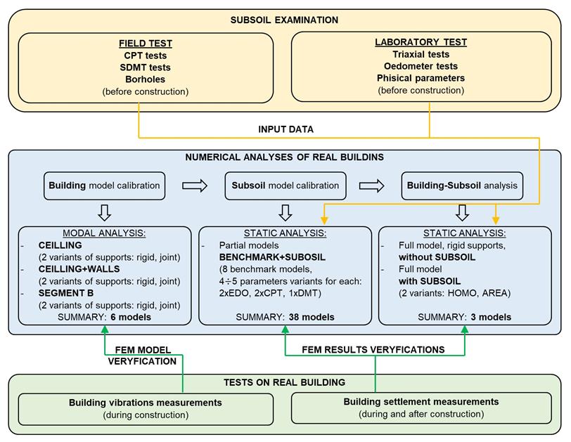
Figure 2.
The soil stiffness degradation curve.
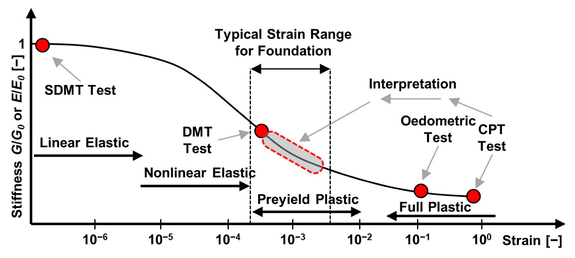
Figure 3.
The analyzed building: (a) view of the real object [33]; (b) map with the location of geotechnical tests (CPT and SDMT), benchmarks (Z1 ÷ Z10) and division into computational areas (A ÷ E).
Figure 3.
The analyzed building: (a) view of the real object [33]; (b) map with the location of geotechnical tests (CPT and SDMT), benchmarks (Z1 ÷ Z10) and division into computational areas (A ÷ E).
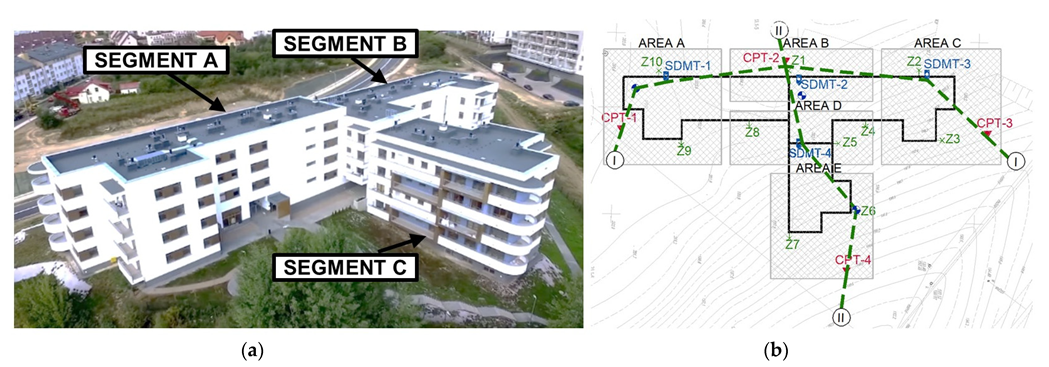
Figure 4.
A geological map of the research area.
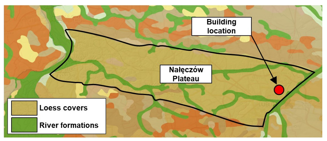
Figure 5.
CPT-1 parameters.
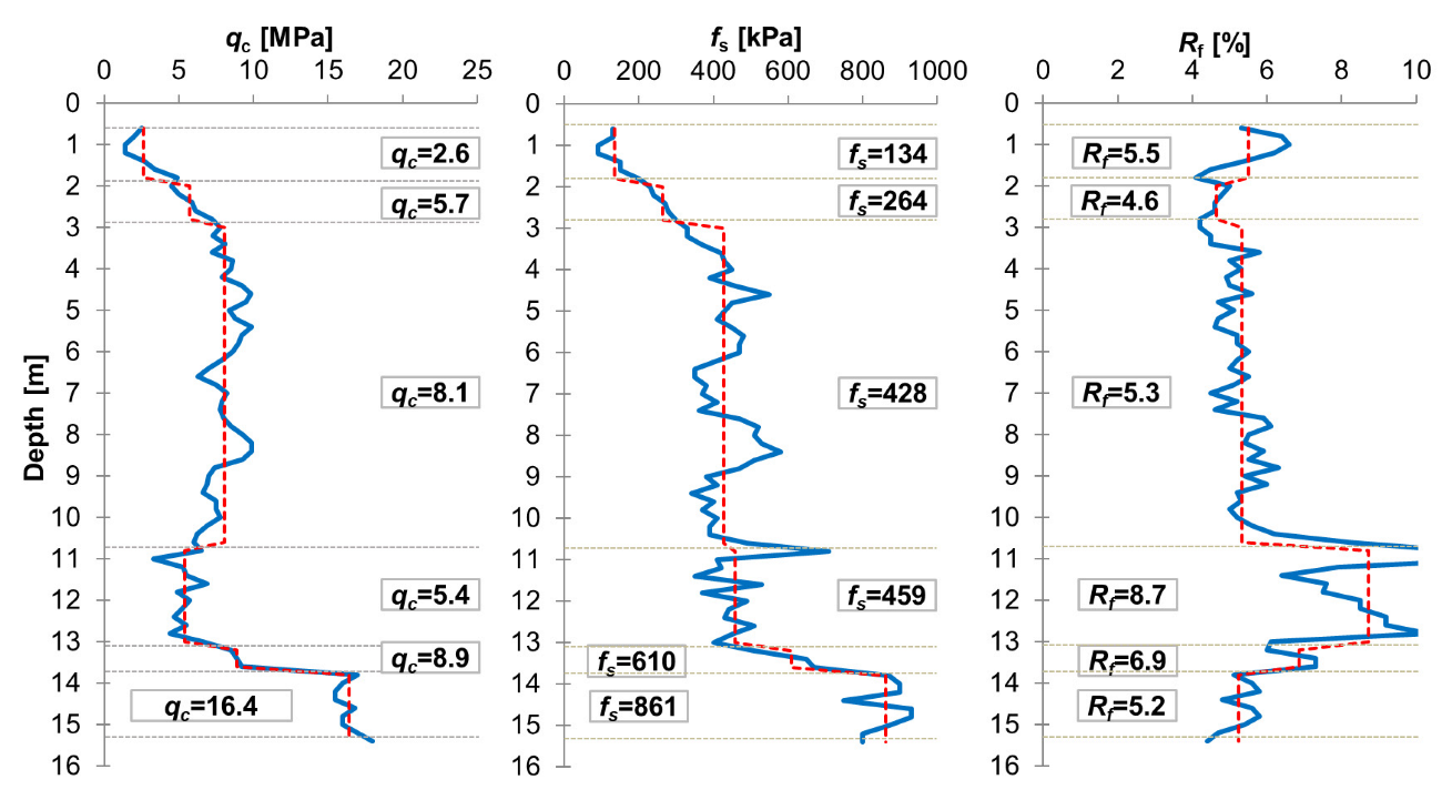
Figure 6.
KD and MDMT distribution with depth (red line—foundation level).

Figure 7.
Laboratory test results (a) oedometric test—sample no. 1; (b) TXCID results on the p-q plane.
Figure 7.
Laboratory test results (a) oedometric test—sample no. 1; (b) TXCID results on the p-q plane.

Figure 8.
Geotechnical cross-sections.
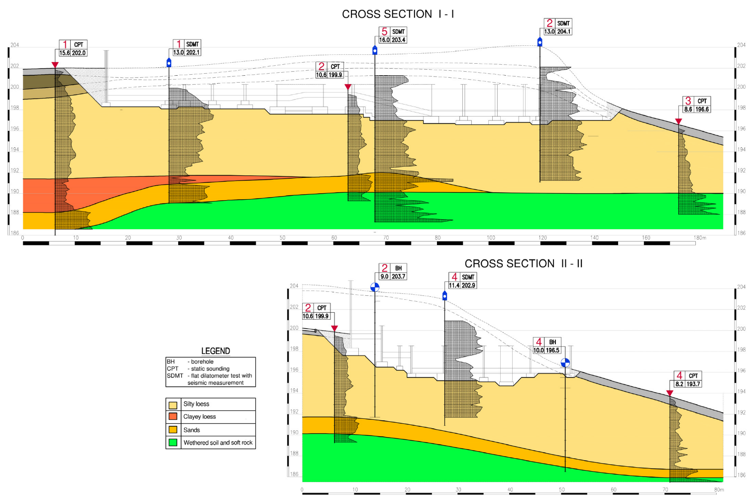
Figure 9.
The course of settlement of benchmarks over time.
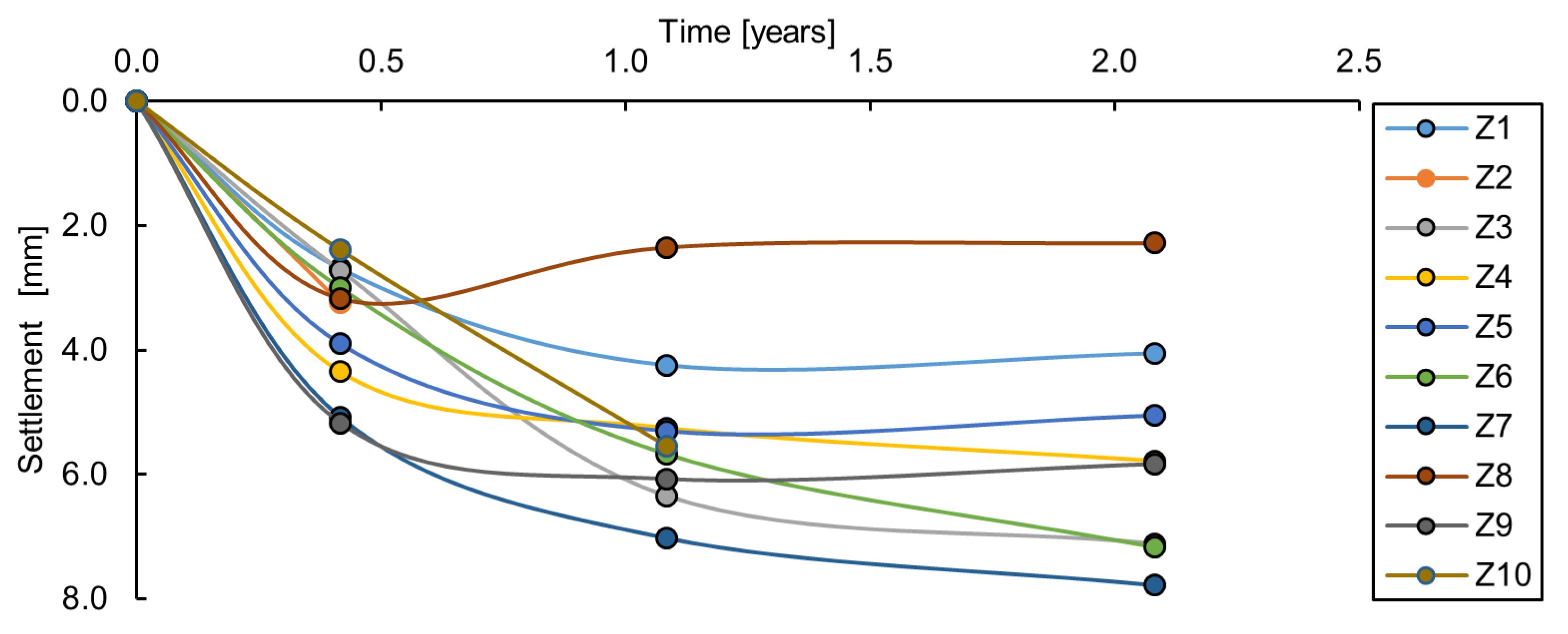
Figure 10.
Assumptions of the Modified Cam-Clay model: (a) p’-e plane; (b) p-q plane.

Figure 11.
Preconsolidation stress determined in oedometric tests (sample No. 3).
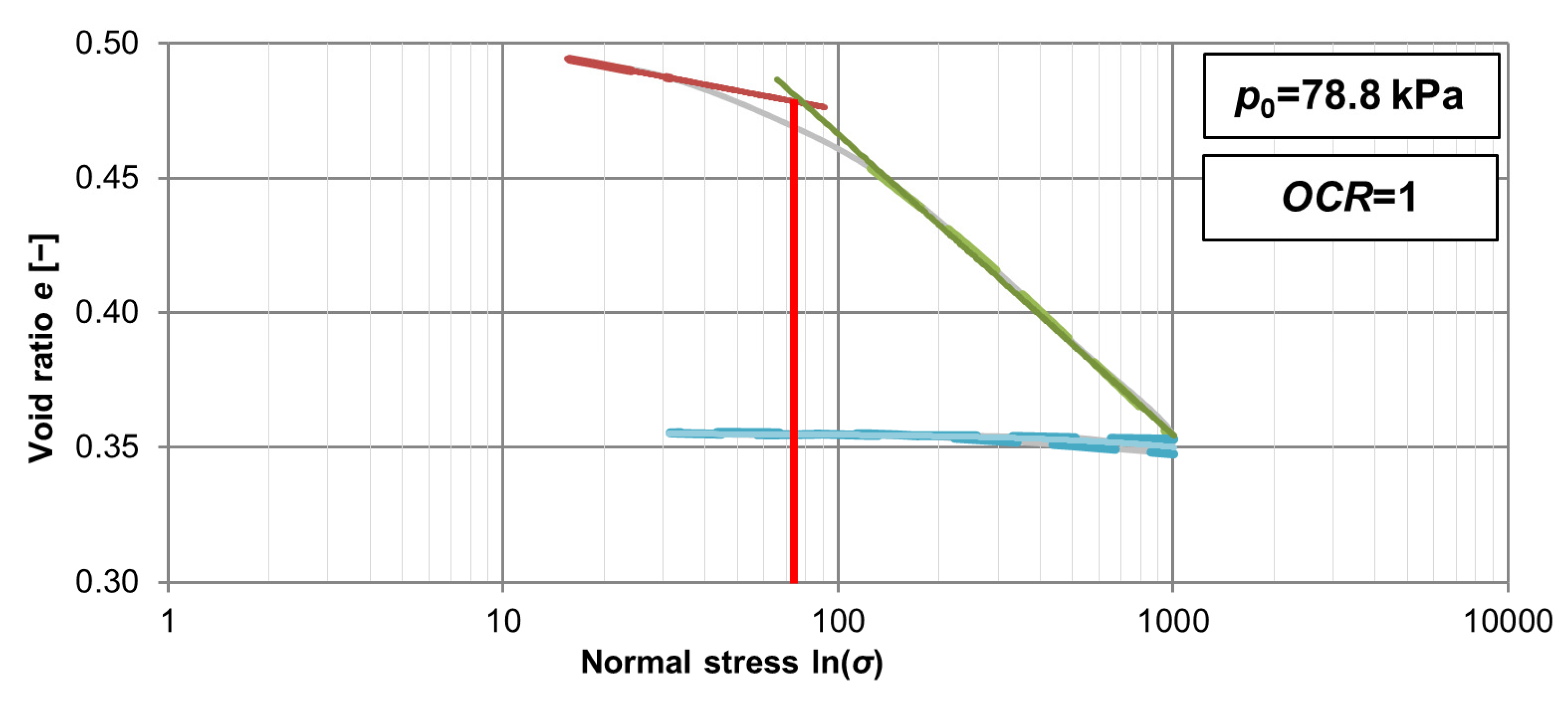
Figure 12.
A scheme showing extraction of the partial calibration models.
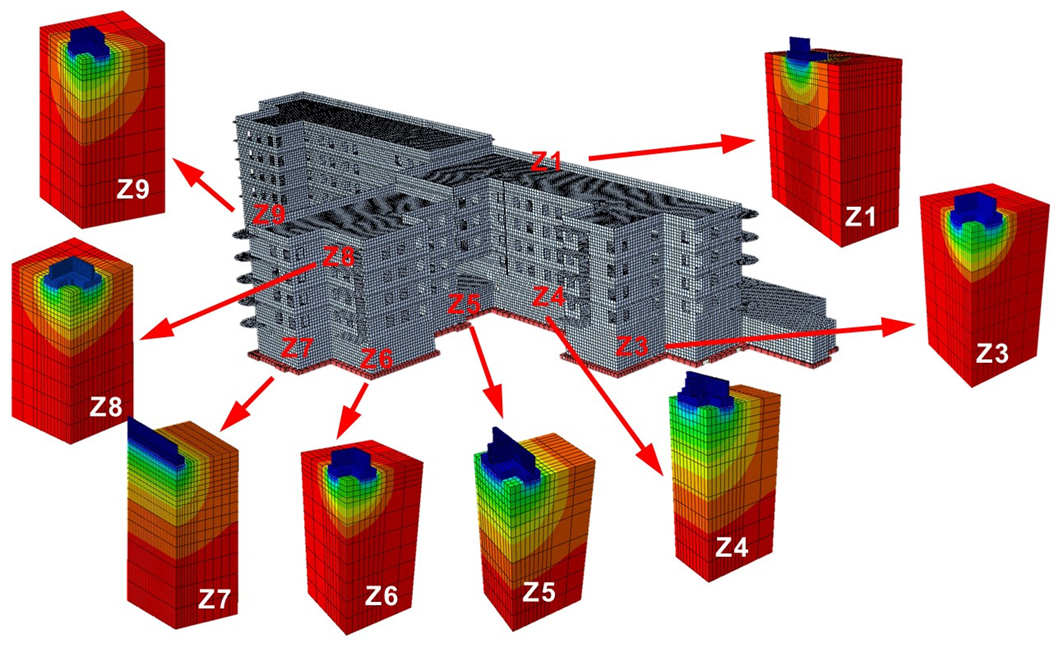
Figure 13.
The partial model Z1—section of the building with the subsoil at the Z1 benchmark: (a) with division into layers, (b) vertical displacement map, (c) S33 stress map—“Geostatic” step, (d) S33 stress map—“Load 3” step.
Figure 13.
The partial model Z1—section of the building with the subsoil at the Z1 benchmark: (a) with division into layers, (b) vertical displacement map, (c) S33 stress map—“Geostatic” step, (d) S33 stress map—“Load 3” step.
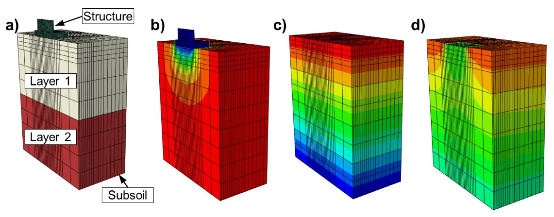
Figure 14.
The division of the subsoil into computational areas.
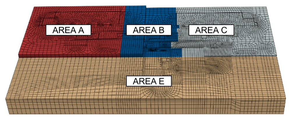
Figure 15.
Vertical displacements in selected subsequent calculation steps [m]: (a) construction of the underground floor, (b) stage of construction at measurement 1, (c) stage after finishing the construction.
Figure 15.
Vertical displacements in selected subsequent calculation steps [m]: (a) construction of the underground floor, (b) stage of construction at measurement 1, (c) stage after finishing the construction.

Figure 16.
Maps of final vertical displacements [m]: (a) RIGID model, (b) AREA model.
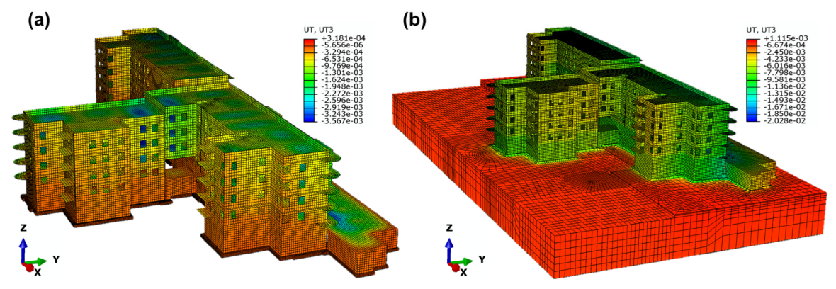
Figure 17.
A map of vertical displacements [m] in a cross-section of the building in the AREA variant.
Figure 17.
A map of vertical displacements [m] in a cross-section of the building in the AREA variant.
Figure 18.
Settlement [mm] change with depth [m] for the benchmarks z-axis in AREA variant (total displacements).
Figure 18.
Settlement [mm] change with depth [m] for the benchmarks z-axis in AREA variant (total displacements).
Figure 19.
Displacement [m] of the building in the expansion joints between segments B and C for the AREA and RIGID models.
Figure 19.
Displacement [m] of the building in the expansion joints between segments B and C for the AREA and RIGID models.
Figure 20.
A comparison of maps of resultant displacements [m] of the building in the AREA (left) and HOMO (right) models.
Figure 20.
A comparison of maps of resultant displacements [m] of the building in the AREA (left) and HOMO (right) models.

Figure 21.
Comparison of the minimum principal stress maps [kPa] of the building in the AREA and RIGID models.
Figure 21.
Comparison of the minimum principal stress maps [kPa] of the building in the AREA and RIGID models.
Figure 22.
A comparison of the minimum principal stress maps [kPa] at the garage entrance in segment A in the AREA and RIGID models.
Figure 22.
A comparison of the minimum principal stress maps [kPa] at the garage entrance in segment A in the AREA and RIGID models.

Figure 23.
A comparison of the maximum principal stress maps [kPa] in a selected reinforced concrete deep beam of segment A in the AREA and RIGID models.
Figure 23.
A comparison of the maximum principal stress maps [kPa] in a selected reinforced concrete deep beam of segment A in the AREA and RIGID models.

Table 1.
Stages of geodetic measurements and loads for the numerical model.
| Phase | Date of the Measurement | Period Since the “Zero” Measurement | Stage of Construction | Description of Loads for the Numerical Model | ||
|---|---|---|---|---|---|---|
| 0 | 05.2014 | 0 | SEGMENT A ceiling above the first floor | SEGMENT B ceiling above the ground floor | SEGMENT C ceiling above the ground floor and walls of the floor | Dead load,
|
| 1 | 10.2014 | 5 months | Construction works finished | Dead load,
| ||
| 2 | 07.2015 | 14 months | The building completed and commissioned | Dead load, load on internal ceilings:
| ||
| 3 | 07.2016 | 26 months | Building used for 1 year | Dead load, load on internal ceilings:
| ||
Table 2.
A compilation of the output parameters of the Modified Cam-Clay model from laboratory tests.
Table 2.
A compilation of the output parameters of the Modified Cam-Clay model from laboratory tests.
| Parameter | λ | κ | M | a0 | p0 | e1 | e0 |
|---|---|---|---|---|---|---|---|
| Sample 1 | 0.0586 | 0.0017 | 1.495 | 37.0 | 84.4 | 0.638 | 0.378 |
| Sample 2 | 0.0607 | 0.0012 | 1.495 | 33.1 | 72.1 | 0.538 | 0.278 |
| Sample 3 | 0.0485 | 0.0015 | 1.495 | 34.4 | 78.8 | 0.567 | 0.356 |
| Mean: | 0.0561 | 0.0015 | 1.495 | 34.5 | 77.4 | 0.584 | 0.340 |
Table 3.
Variants of subsoil parameters in the Modified Cam-Clay model.
| Variant | Description |
|---|---|
| EDO1 | Compressibility parameters from oedometric tests. Homogeneous subsoil. |
| EDO2 | Compressibility parameters from oedometric tests—modified. Homogeneous subsoil. |
| CPT1 | Initial compressibility parameters from CPT tests. Homogeneous subsoil. |
| CPT2 | Initial compressibility parameters from CPT tests. Layered subsoil. |
| DMT | Initial compressibility parameters from SDMT tests. Homogeneous subsoil. |
Table 4.
A compilation of the parameters of the Modified Cam-Clay model for partial models.
| Partial Model | Variant | Subsoil Layer | Cam-Clay Model Parameters | ||||||
|---|---|---|---|---|---|---|---|---|---|
| λ | κ | M | a0 | p0 | e1 | e0 | |||
| Z1 | EDO1 | 1 | 0.0561 | 0.0014 | 1.495 | 34.5 | 95 | 0.584 | 0.340 |
| EDO2 | 1 | 0.0512 | 0.0004 | 1.495 | 39.1 | 95 | 0.567 | 0.342 | |
| CPT1 | 1 | 0.0071 | 0.0014 | 1.495 | 19.3 | 95 | 0.584 | 0.552 | |
| CPT2 | 1 | 0.0071 | 0.0014 | 1.495 | 19.3 | 95 | 0.584 | 0.552 | |
| 2 | 0.0040 | 0.0014 | 1.495 | 13.1 | 209 | 0.584 | 0.565 | ||
| DMT | 1 | 0.0078 | 0.0014 | 1.495 | 20.9 | 95 | 0.584 | 0.548 | |
| Z3 | EDO1 | 1 | 0.0561 | 0.0014 | 1.495 | 35.3 | 38 | 0.584 | 0.340 |
| EDO2 | 1 | 0.0512 | 0.0004 | 1.495 | 39.4 | 38 | 0.567 | 0.342 | |
| CPT1 | 1 | 0.0075 | 0.0014 | 1.495 | 9.9 | 38 | 0.584 | 0.556 | |
| CPT2 | 1 | 0.0112 | 0.0014 | 1.495 | 9.9 | 38 | 0.584 | 0.556 | |
| 2 | 0.0075 | 0.0014 | 1.495 | 16.1 | 78 | 0.584 | 0.554 | ||
| 3 | 0.0034 | 0.0014 | 1.495 | 8.6 | 98 | 0.584 | 0.567 | ||
| DMT | 1 | 0.0052 | 0.0014 | 1.495 | 7.1 | 38 | 0.584 | 0.565 | |
| Z4 | EDO1 | 1 | 0.0561 | 0.0014 | 1.495 | 34.4 | 114 | 0.584 | 0.340 |
| EDO2 | 1 | 0.0512 | 0.0004 | 1.495 | 39.0 | 114 | 0.567 | 0.342 | |
| CPT1 | 1 | 0.0071 | 0.0014 | 1.495 | 25.1 | 114 | 0.584 | 0.546 | |
| CPT2 | 1 | 0.0071 | 0.0014 | 1.495 | 25.1 | 114 | 0.584 | 0.546 | |
| 2 | 0.0040 | 0.0014 | 1.495 | 10.8 | 152 | 0.584 | 0.566 | ||
| 3 | 0.0034 | 0.0014 | 1.495 | 25.4 | 182 | 0.584 | 0.554 | ||
| DMT | 1 | 0.0064 | 0.0014 | 1.495 | 20.2 | 114 | 0.584 | 0.554 | |
| Z5 | EDO1 | 1 | 0.0561 | 0.0014 | 1.495 | 34.7 | 76 | 0.584 | 0.340 |
| EDO2 | 1 | 0.0512 | 0.0004 | 1.495 | 39.1 | 76 | 0.567 | 0.342 | |
| CPT1 | 1 | 0.0071 | 0.0014 | 1.495 | 18.0 | 76 | 0.584 | 0.549 | |
| CPT2 | 1 | 0.0071 | 0.0014 | 1.495 | 18.0 | 76 | 0.584 | 0.549 | |
| 2 | 0.0040 | 0.0014 | 1.495 | 9.0 | 114 | 0.584 | 0.567 | ||
| DMT | 1 | 0.0064 | 0.0014 | 1.495 | 14.7 | 76 | 0.584 | 0.556 | |
| Z6 | EDO1 | 1 | 0.0561 | 0.0014 | 1.495 | 35.9 | 19 | 0.584 | 0.340 |
| EDO2 | 1 | 0.0512 | 0.0004 | 1.495 | 39.6 | 19 | 0.567 | 0.342 | |
| CPT1 | 1 | 0.0095 | 0.0014 | 1.495 | 6.0 | 19 | 0.584 | 0.558 | |
| CPT2 | 1 | 0.0095 | 0.0014 | 1.495 | 6.0 | 19 | 0.584 | 0.558 | |
| 2 | 0.0037 | 0.0014 | 1.495 | 9.9 | 133 | 0.584 | 0.566 | ||
| Z7 | EDO1 | 1 | 0.0561 | 0.0014 | 1.495 | 35.9 | 19 | 0.584 | 0.340 |
| EDO2 | 1 | 0.0512 | 0.0004 | 1.495 | 39.6 | 19 | 0.567 | 0.342 | |
| CPT1 | 1 | 0.0095 | 0.0014 | 1.495 | 6.0 | 19 | 0.584 | 0.558 | |
| CPT2 | 1 | 0.0095 | 0.0014 | 1.495 | 6.0 | 19 | 0.584 | 0.558 | |
| 2 | 0.0037 | 0.0014 | 1.495 | 9.9 | 133 | 0.584 | 0.566 | ||
| Z8 | EDO1 | 1 | 0.0561 | 0.0014 | 1.495 | 34.5 | 95 | 0.584 | 0.340 |
| EDO2 | 1 | 0.0512 | 0.0004 | 1.495 | 39.1 | 95 | 0.567 | 0.342 | |
| CPT1 | 1 | 0.0071 | 0.0014 | 1.495 | 20.9 | 95 | 0.584 | 0.548 | |
| CPT2 | 1 | 0.0071 | 0.0014 | 1.495 | 20.9 | 95 | 0.584 | 0.548 | |
| 2 | 0.0040 | 0.0014 | 1.495 | 24.6 | 133 | 0.584 | 0.550 | ||
| DMT | 1 | 0.0064 | 0.0014 | 1.495 | 17.5 | 95 | 0.584 | 0.555 | |
| Z9 | EDO1 | 1 | 0.0561 | 0.0014 | 1.495 | 34.7 | 76 | 0.584 | 0.340 |
| EDO2 | 1 | 0.0512 | 0.0004 | 1.495 | 39.1 | 76 | 0.567 | 0.342 | |
| CPT1 | 1 | 0.0052 | 0.0014 | 1.495 | 12.3 | 76 | 0.584 | 0.561 | |
| CPT2 | 1 | 0.0052 | 0.0014 | 1.495 | 12.3 | 76 | 0.584 | 0.561 | |
| 2 | 0.0080 | 0.0014 | 1.495 | 33.0 | 209 | 0.584 | 0.549 | ||
| DMT | 1 | 0.0064 | 0.0014 | 1.495 | 14.7 | 76 | 0.584 | 0.556 | |
Table 5.
A comparison of the final settlements and settlements calculated for partial models.
| Partial Model (Benchmark) | Mean | ||||||||||
|---|---|---|---|---|---|---|---|---|---|---|---|
| Z1 | Z3 | Z4 | Z5 | Z6 | Z7 | Z8 | Z9 | ||||
| Actual settlement | 4.0 | 7.1 | 5.8 | 5.1 | 7.2 | 7.8 | 2.3 | 5.8 | |||
| Calculated settlement | s [mm] | EDO1 | 42.9 | 45.5 | 19.7 | 10.6 | 38.3 | 49.4 | 7.1 | 28.1 | |
| EDO2 | 39.4 | 24.7 | 15.7 | 6.4 | 21.9 | 32.5 | 6.6 | 12.9 | |||
| CPT1 | 6.9 | 13.8 | 5.1 | 3.3 | 14.7 | 16.7 | 2.0 | 2.8 | |||
| CPT2 | 6.9 | 9.8 | 5.1 | 3.2 | 14.7 | 16.2 | 2.0 | 2.8 | |||
| DMT | 7.3 | 6.6 | 4.6 | 3.0 | - | - | 1.8 | 3.1 | |||
| Absolute calculation error | Δs [mm] | EDO1 | 38.9 | 38.4 | 13.9 | 5.6 | 31.1 | 41.6 | 4.8 | 22.3 | |
| EDO2 | 35.4 | 17.6 | 9.9 | 1.4 | 14.7 | 24.7 | 4.3 | 7.1 | |||
| CPT1 | 2.9 | 6.7 | −0.7 | −1.8 | 7.5 | 8.9 | −0.3 | −3.0 | |||
| CPT2 | 2.9 | 2.7 | −0.7 | −1.9 | 7.5 | 8.4 | −0.3 | −3.0 | |||
| DMT | 3.3 | −0.5 | −1.2 | −2.1 | - | - | −0.5 | −2.7 | |||
| Relative error | δ [%] | EDO1 | 77.7 | 76.8 | 27.8 | 11.1 | 62.3 | 83.2 | 9.6 | 44.5 | 49.1 |
| EDO2 | 70.7 | 35.2 | 19.8 | 2.7 | 29.5 | 49.4 | 8.6 | 14.1 | 28.8 | ||
| CPT1 | 5.7 | 13.4 | −1.4 | −3.5 | 15.1 | 17.8 | −0.6 | −6.1 | 7.9 | ||
| CPT2 | 5.7 | 5.4 | −1.4 | −3.7 | 15.1 | 16.8 | −0.6 | −6.1 | 6.8 | ||
| DMT | 6.5 | −1.0 | −2.4 | −4.1 | - | - | −1.0 | −5.5 | 3.4 | ||
Table 6.
Derived Modified Cam-Clay parameters for the full building-subsoil model.
| Variant | λ | κ | M | a0 | p0 | e1 | e0 | |
|---|---|---|---|---|---|---|---|---|
| HOMO | 0.0069 | 0.0014 | 1.495 | 12.0 | 59.0 | 0.584 | 0.557 | |
| AREA | AREA A | 0.0054 | 0.0014 | 1.495 | 12.3 | 76.0 | 0.584 | 0.561 |
| AREA B + D | 0.0071 | 0.0014 | 1.495 | 19.3 | 95.0 | 0.584 | 0.552 | |
| AREA C | 0.0078 | 0.0014 | 1.495 | 9.9 | 38.0 | 0.584 | 0.556 | |
| AREA E | 0.0090 | 0.0014 | 1.495 | 6.0 | 19.0 | 0.584 | 0.558 | |
Table 7.
A comparison of final settlements and settlements calculated [mm] for full models.
| FULL MODEL OF THE BUILDING + SUBSOIL (HOMO) | ||||||||||
| Phase | Z1 | Z3 | Z4 | Z5 | Z6 | Z7 | Z8 | Z9 | Mean | |
| 1 | 4.1 | 2.3 | 4.5 | 2.5 | 1.7 | 2.4 | 4.9 | 3.5 | 3.2 | |
| 2 | 7.7 | 4.0 | 8.2 | 3.8 | 2.1 | 3.3 | 8.9 | 6.0 | 5.5 | |
| 3 | 8.8 | 4.6 | 9.3 | 4.2 | 2.2 | 3.5 | 10.2 | 6.8 | 6.2 | |
| FULL MODEL OF THE BUILDING + SUBSOIL (AREA) | ||||||||||
| Phase | Z1 | Z3 | Z4 | Z5 | Z6 | Z7 | Z8 | Z9 | Mean | |
| 1 | 4.9 | 2.0 | 5.7 | 3.0 | 2.0 | 2.8 | 2.8 | 2.3 | 3.2 | |
| 2 | 9.3 | 3.3 | 10.7 | 5.1 | 2.9 | 4.0 | 5.1 | 3.9 | 5.5 | |
| 3 | 10.5 | 3.7 | 12.1 | 5.7 | 3.2 | 4.4 | 6.0 | 4.4 | 6.2 | |
| ACTUAL SETTLEMENT | ||||||||||
| Phase | Z1 | Z3 | Z4 | Z5 | Z6 | Z7 | Z8 | Z9 | Mean | |
| 1 | 2.7 | 2.7 | 4.3 | 3.9 | 3.0 | 5.1 | 3.2 | 5.2 | 3.6 | |
| 2 | 4.2 | 6.3 | 5.2 | 5.3 | 5.7 | 7.0 | 2.3 | 6.1 | 5.3 | |
| 3 | 4.0 | 7.1 | 5.8 | 5.1 | 7.2 | 7.8 | 2.3 | 5.8 | 5.6 | |
| CALCULATION ERROR | ||||||||||
| Z1 | Z3 | Z4 | Z5 | Z6 | Z7 | Z8 | Z9 | Mean | ||
| Absolute error [mm] | HOMO | 4.8 | −2.5 | 3.5 | −0.9 | −5.0 | −4.3 | 7.9 | 1.0 | 3.74 |
| AREA | 6.5 | −3.4 | 6.3 | 0.6 | −4.0 | −3.4 | 3.7 | −1.4 | 3.66 | |
| Relative error [%] | HOMO | 9.6 | −5.0 | 7.0 | −1.8 | −10.0 | −8.6 | 15.8 | 2.0 | 7.48 |
| AREA | 13.1 | −6.8 | 12.5 | 1.2 | −8.0 | −6.9 | 7.4 | −2.8 | 7.34 | |
Publisher’s Note: MDPI stays neutral with regard to jurisdictional claims in published maps and institutional affiliations. |
© 2022 by the author. Licensee MDPI, Basel, Switzerland. This article is an open access article distributed under the terms and conditions of the Creative Commons Attribution (CC BY) license (https://creativecommons.org/licenses/by/4.0/).
Share and Cite
MDPI and ACS Style
Nepelski, K. 3D FEM Analysis of the Subsoil-Building Interaction. Appl. Sci. 2022, 12, 10700. https://doi.org/10.3390/app122110700
AMA Style
Nepelski K. 3D FEM Analysis of the Subsoil-Building Interaction. Applied Sciences. 2022; 12(21):10700. https://doi.org/10.3390/app122110700
Chicago/Turabian StyleNepelski, Krzysztof. 2022. "3D FEM Analysis of the Subsoil-Building Interaction" Applied Sciences 12, no. 21: 10700. https://doi.org/10.3390/app122110700
Note that from the first issue of 2016, this journal uses article numbers instead of page numbers. See further details here.