Abstract
The integrity of shoreline is disrupted by cliffs, posing obstacles to marine surveying and chart mapping, particularly in research related to the cliff section of the sea area. The present study proposes a method to solve this problem. In the proposed method, we first extract the boundary of the cliff to segment the point cloud according to a designed rule, then calculate the centroid coordinates of each point cloud block, followed by the coordinates of side points on both sides of the boundary of each block from the centroid, and finally create a side point cloud projected to the water surface corrected for elevation. The corrected point cloud is considered a point cloud dataset of the innermost shoreline. Combined with a point cloud projected from the boundary of the cliff section to the water surface, we developed a calculation method for the optimal shoreline position. Our experiment proved that the method could effectively extract the shoreline of the study area. Moreover, compared with that of the commonly used shoreline extraction method, the absolute error of the isoline tracking method was very large, up to several meters. However, the proposed method achieved smaller standard deviation and variance (0.1254 and 0.0157, respectively) than the isoline tracking method (0.9837 and 0.9677, respectively).
1. Introduction
Shoreline is one of the important linear elements of a chart, and it is closely related to the investigation of national coastal zones, construction of adjacent waters, and protection of the coast, among others. Many researchers have attempted to obtain the total length and exact location of the shoreline through technical measures. At present, shorelines are mainly extracted from two types of data sources: aerial image and LiDAR data. Image data acquisition is easily affected by the environment and climate, among other factors, and the data are often accompanied by shadow areas. Therefore, the accuracy of shorelines extracted from image data is limited, and in the presence of shadow areas, the shoreline cannot be extracted. LiDAR can generate high-precision three-dimensional coordinate data, as well as other auxiliary data, such as laser echo time, echo intensity, and an appropriate flight height and scanning frequency can be set during data collection such that the obtained data have a high density. Moreover, since airborne LiDAR is not easily affected by the environment, it can operate in all weather conditions and offers advantages over aerial imagery, such as the feasibility of application for marine measurements and research, which are key topics in the field. Stockdonf et al. [1] used airborne LiDAR data to estimate the location of and changes in shoreline; however, the authors used only a rough estimation method to extract the shoreline. Robertson et al. [2] proposed a method of shoreline mapping using airborne LiDAR data, summarized as a coastal profile method. Xu et al. [3] used airborne LiDAR data to propose a step-by-step extraction method for the shoreline, as well as an optimization method for the shoreline boundary. Luque et al. [4] used airborne LiDAR data to generate a digital elevation model (DEM) and then processed the DEM to extract the shoreline. Weihua et al. [5] explored the adaptability of an algorithm to various coastal zone data types, and proposed a specific method with high accuracy and adaptability for shoreline extraction in shoals and muddy areas. Based on Monte Carlo simulations, Liu et al. [6] extracted the shoreline using LiDAR data and evaluated its accuracy; the method generates a DEM from LiDAR data, intersects the DEM with the tidal datum, and then separates land and water images. After image processing, mathematical morphology operation, line tracking, and vectorisation, the shoreline data are finally obtained. Furthermore, Incekara et al. [7] used the intensity information in airborne LiDAR data to extract the shoreline; the method first converts the intensity information in the point cloud into an infrared band, and then extracts the shoreline after a certain method design and process. Wei et al. [8] attempted to separate the land and water points in LiDAR data to extract the shoreline; they used terrain, slope, and point density information from the obtained data and combined it with the sample information of land and water. Similarly, Smeeckaert et al. [9] attempted to separate water and land using airborne LiDAR data and by combining the characteristics of ground features. Separating land and water points can provide a better reference for shoreline extraction. In some studies, LiDAR data were combined with image data to extract shorelines. For instance, Yousef et al. [10] combined point cloud and image data, detected and removed outliers through morphological methods, and removed artificial facilities, such as ports, outside the shoreline through Hough transformation; this method requires DEM from point cloud data. Nu et al. [11] combined point clouds and images to extract the boundaries of a lake. Sukcharoenpong et al. [12] extracted the shoreline through the fusion of hyperspectral images and generated a DEM based on LiDAR data. First, a preliminary solution was obtained, and then the shoreline was extracted using contour evolution technology. In addition, some studies [13,14,15,16] have used airborne LiDAR data to estimate and analyze the location of the shoreline and then evaluated other marine elements, such as coastal protection and wind force. Although these studies did not use airborne LiDAR data to extract the shoreline, they used the shoreline obtained from an LiDAR data source to examine other marine elements. From these reports, airborne LiDAR data play an important role in shoreline extraction and other aspects of oceanic research.
From the above literature, a majority of the shoreline extraction methods have used point cloud data to first generate a DEM; however, DEM construction is a very time-consuming and error-prone process, and the accuracy of shoreline extraction through DEM is low [17,18,19]. Moreover, when data distribution characteristics do not match, the algorithm fails. Therefore, many effective and reliable extraction algorithms suitable for specific shoreline types have been proposed through analyses of data characteristics of each type. Bengoufa et al. [20] proposed the use of deep learning and object-oriented analysis for bedrock shoreline extraction. Weifu et al. [21] established different interpretation marks according to different shoreline types using remote sensing data and designed different shoreline extraction methods. However, these studies did not examine the extraction of all shoreline types, but rather proposed a targeted method for the extraction of a specific shoreline type, because it is difficult to develop an effective algorithm that can adapt to all data types for all shoreline types. There have been no reliable extraction methods using image or point cloud data for sheltered shorelines at cliffs or under big rocks. However, these types account for a certain proportion of shorelines, and the entire shoreline cannot be extracted because of the lack of this type. To this end, to analyze the characteristics of sheltered shorelines, this study proposes an effective and efficient extraction method combining force characteristics and point cloud segmentation.
2. Methods
2.1. Data Introduction and Method Flow
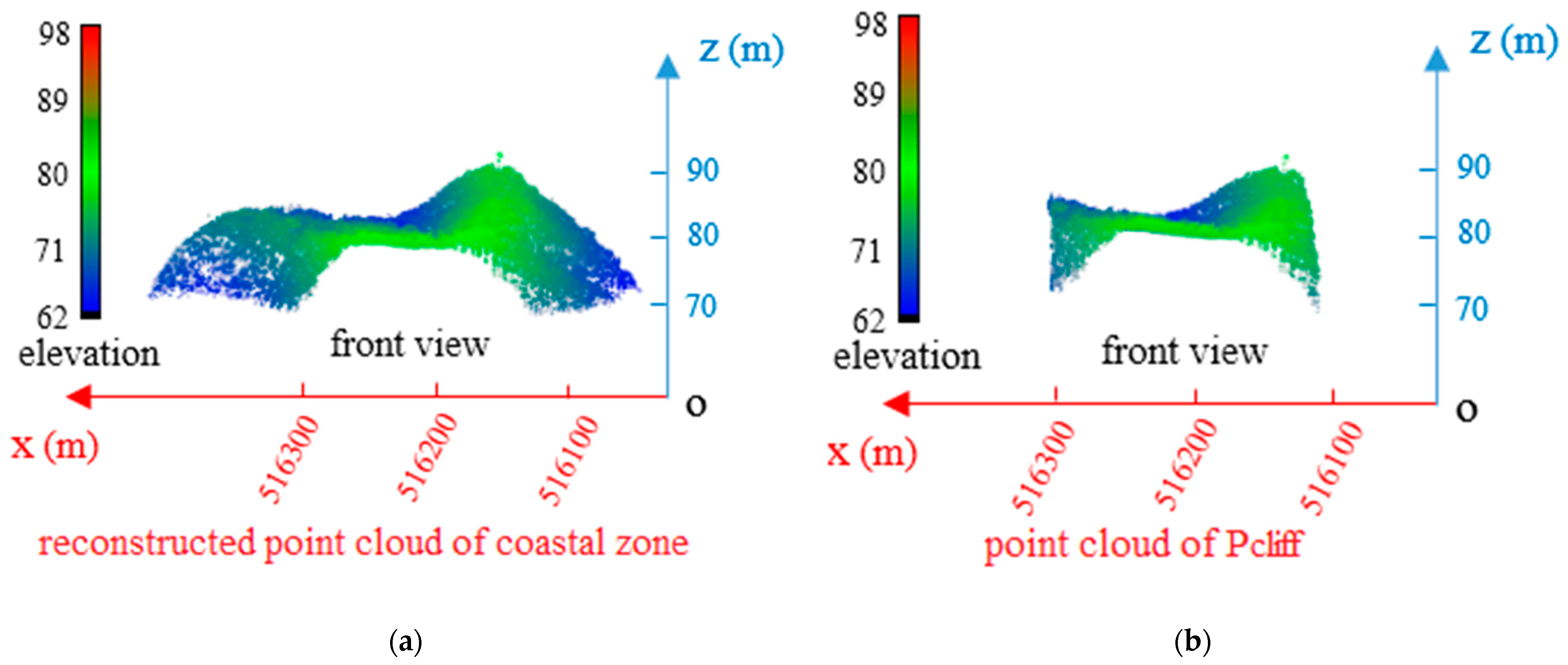
A typical sea area in Longkou City, Shandong Province, China, was selected as the experimental object. The data size is 165 MB with a total of 5,922,266 points. The lower left coordinate is x = 516,728, y = 3,372,488.2, z = 89.639999; the upper right coordinate is x = 510,528.21, y = 3,370,108.7, z = 72.589996. These coordinates are coordinates under the space rectangular coordinate system. The coordinate origin of the space rectangular coordinate system is located at the center of the reference ellipsoid, the Z-axis points to the north pole of the reference ellipsoid, the X-axis points to the intersection of the starting meridian plane and the equator, and the Y-axis is located on the equator plane and forms a 90° on the X-axis with the right hand system. Each point contains three-dimensional coordinate information, echo intensity, and echo times information. The original image is shown in Figure 1a, in which the red box shows the coastal zone area composed of a larger cliff area. The size of this cliff area data file is 11.196 MB, with a total of 405,650 points. The point cloud image is shown in Figure 1b.

Figure 1.
(a) The image of point cloud in original sea area; (b) the image of point cloud in cliff area.
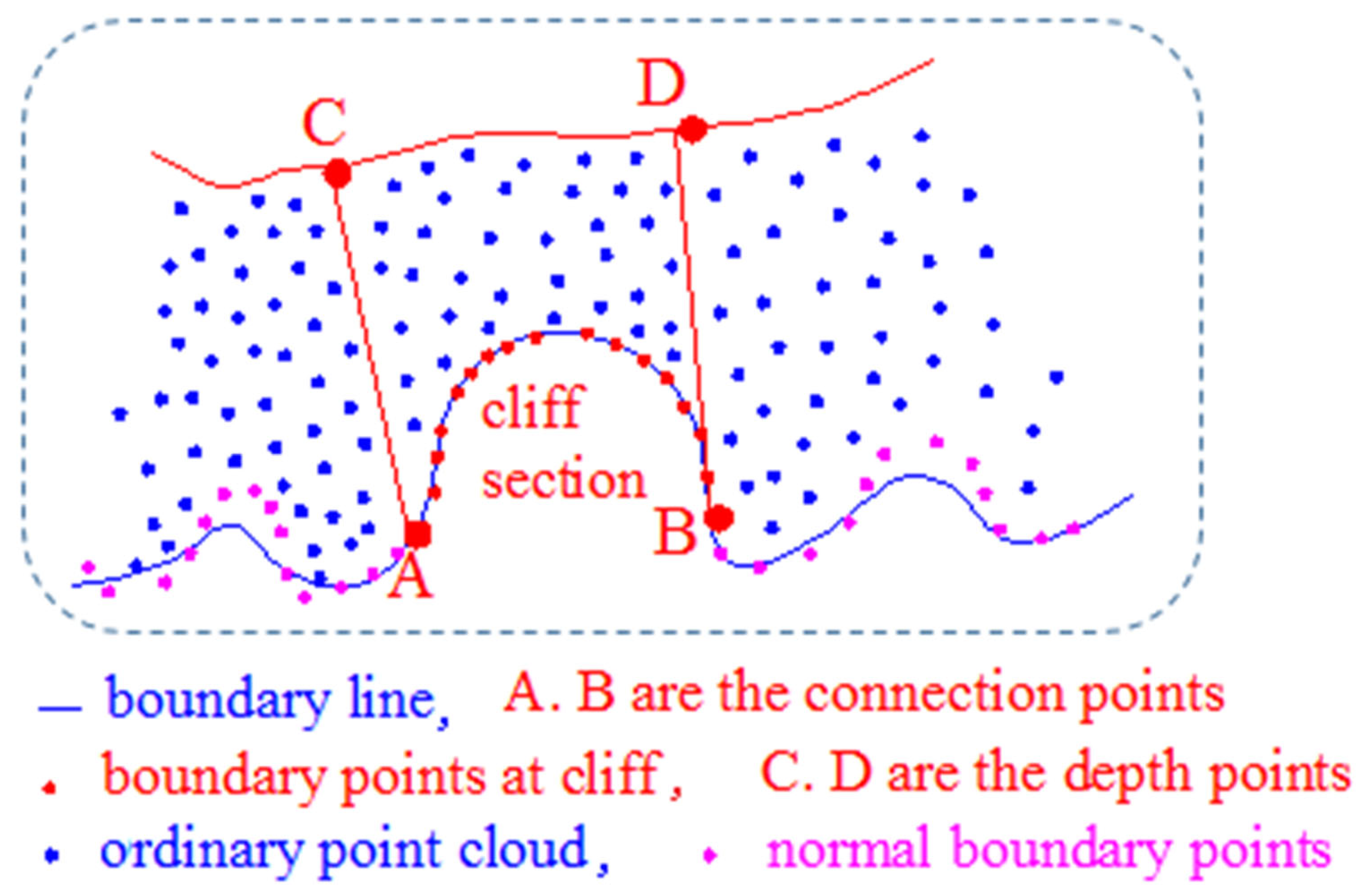
Three concepts are defined here. (1) Connection points. The outer line of the point cloud in the sea area, which includes the cliff section, is the process of passing through the outer line of the normal ground, then passing through the transition point to the outer line of the cliff section, and then passing through the transition point on the other side to return to the outer line of the normal ground. These two transition points, the two points connecting the outer line of the ordinary ground and the outer line of the cliff section, are called “connection points”. (2) Depth points. From the outer line of the cliff section, the ground of the cliff section will be lowered from the water body side to the land side (in this case, the ground of the cliff section will be lowered from the land side to the water body side, which is almost non-existent in practice). When the ground elevation is lowered to approximately the same height as the water body, the ground at this time is considered as the last position of the cliff section. This position can be divided by a line, which is imaginary in the data. However, the ground of the cliff section will decrease from the water body side to the land side; that is, the elevation of the ground will decrease. The ground is lowered to approximately the same height as the water body; that is, the elevation of the ground is close to the elevation of the two connection points. Therefore, the point with the smallest difference between the two connection points in the x, y plane direction and the z elevation direction can be found in the cliff section area data, and these two points are called “depth points”. (3) Side points. The point cloud of the cliff segment is segmented at fixed intervals according to the x-coordinate (x-coordinate when the main coastline is east-west or west-east, and y-coordinate when the main coastline is north-south or south-north). Each segment is called a point-cloud block, and the centroid coordinates of each point-cloud block are calculated. Each block can be imagined as a rectangle. Take the coastline whose main trend is along the x-axis as an example; the short side of the rectangle (that is, the block spacing) is parallel to the x-axis, and the long side is parallel to the y-axis. Only the x and y coordinates of the point cloud in the block are considered. It can be imagined that the plane coordinates of these points are all within the rectangle. Then, the parallel line to the short side of the rectangle is made through the plane coordinates of the centroid point of the block. Then, the line is parallel to the short side and also parallel to the x-axis. The parallel line will have two intersection points with the two long sides of the rectangle. These two intersections are called “side points”.
The main process is now discussed. First, the boundary of the point cloud toward the sea in the cliff area was extracted. Then, the connection points between the cliff and ordinary segments were extracted using the designed method, and the depth points were calculated. Finally, the point cloud of the cliff area was accurately extracted. Using the point cloud of each block in the cliff according to the x-coordinate, the centroid of the point cloud in each block was calculated, followed by the coordinates of the side points on both sides of the block derived from the centroid coordinates. The side points were then projected onto the water surface, and the elevation was corrected. Subsequently, the boundary of the cliff section was projected onto the water surface. The optimal coastline at the cliff according to the two projected point clouds was calculated using the proposed method. The general process is illustrated in Figure 2.
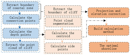
Figure 2.
The methodological flow chart.
2.2. Point Cloud Extraction at the Cliff
The point cloud extraction at the cliff is now defined. Here, represents a point cloud dataset, represents a point cloud dataset named text, and represents the point with number of i in the dataset, represents the coordinates of the point, represents the echo intensity of the point, and is the number of echoes of the point.
For the coastal zone data form, as shown in Figure 1b, the boundary point cloud dataset was obtained using the extraction method, provided in the literature [5], in which edge points were extracted based on the distribution rule of acquired data during airborne lidar scanning. The distribution rule is roughly as follows: the x or y coordinates of the points will change from small to large, then from large to small, and then from small to large with the scanning line. The point cloud dataset of the boundary was set as , which contains both the boundary points of the normal coastal zone and those near the sea at the cliff. There were two special transition points at the intersection of these two types of boundary point clouds, points A and B (Figure 3). These two points connect the boundary point set of the normal coastal zone to the edge point set of the cliff, and then again to the boundary point set of the normal coastal zone. For the boundary point cloud of the normal coastal zone, the elevation difference between two adjacent points was relatively small, and the maximum elevation difference was approximately 10 cm. As such, when point A was reached, the elevation of the point next to A was much higher than that of point A, and then the elevation of the point increased. When the point reached the top, the elevation decreased. Once it was reduced to junction point B, the elevation change of the point was small, and it transited to the boundary point cloud of the normal shoreline. Because the magnitude of the elevation changes of points was not easy to determine, the change ratio of the difference in elevation between the rear and current points, and that between the front and current points, was evident. Therefore, the corresponding judgment rules can be set according to this feature to find points A and B.
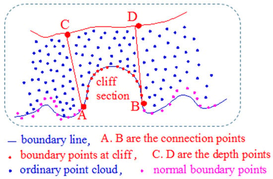
Figure 3.
Schematic diagram of the extraction of point cloud at cliff.
First, the original coastal zone data is imported into existing point cloud processing software to determine the primary information of the approximate trend of the coastline. If the coastline is mainly east-west or west-east, the points in are sorted from small to large by the x coordinate; if the x coordinate is the same, the points are sorted from small to large by the y coordinate; if x and y are the same, the points are sorted from small to large by the z coordinate. If the coastline is mainly north-south or south-north, the points in the are sorted from small to large by y-coordinate. If the y-coordinate is the same, the points are sorted from small to large using the x-coordinate. If x and y are the same, the points are sorted from small to large according to the z-coordinate, and the first and last points are removed.
The following relevant processing methods take the coastline which is roughly east-west or west-east, as a model. If the coastline is roughly north-south or north-south, the x- and y-coordinates are accordingly adjusted. The following equation was applied and calculation was performed:
where, N is the total number of points in .
When the value of is close to one, it can be regarded as the boundary point of the normal coastline. For the two connecting points A and B, the value of one point should be larger, usually greater than 2, and that of the other point should be smaller, approaching 0. Therefore, when the value of is greater than 2 or tends toward 0, the point can be extracted, and then the extracted point can be either point A or B in Figure 3. For the extraction of point cloud on the cliff, the intercepted depth H must be determined, which can be obtained by first finding the two points C and D that are the closest to the x coordinates (y coordinates, when the coastline is roughly south-north or north-south) of A and B, and their elevation is also the closest to the elevation of A and B. First, the two points C and D are determined according to strict conditions, the distance between AC and BD is calculated, and then the average of the distances between AC and BD is calculated. This value is the intercepted depth H. With the limitation of the x coordinate interval of points A and B, combined with the depth parameter H, the point cloud of the coastal zone at the cliff can be accurately extracted, assuming that this point cloud dataset is .
2.3. Point Cloud Segmentation at the Cliff
Assume that the coastline is mainly in an east-west or an west-east direction. The point cloud dataset at the cliff is sorted by the x coordinate from small to large. Starting from the x coordinate of the first point, points with a fixed value difference from the x coordinate of the first point are classified as a single point cloud dataset and recorded as , where the x coordinate between and is recorded as the second type, and the point cloud is recorded as . By analogy, all points in are divided into many separate point clusters according to the x coordinate.
The process of point cloud blocking is presented in Figure 4.
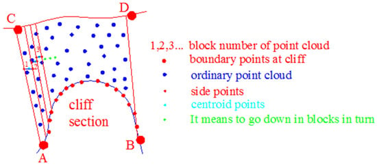
Figure 4.
The schematic diagram of point cloud segmentation, centroid points, and side points.
2.4. Calculation of Centroid Points of Each Block and Side Points
Because soil at the cliff and ground objects on the soil require bearing capacity support, that is, the bottom of the cliff near the sea side is mostly hollowed out and there is less ground object support in the vertical direction, the possible location of the support under the cliff must be determined. According to the analysis of terrain characteristics and the supporting effect of force on the cliff, supports under the cliff can be offset from the vertical direction under the cliff to the land side. According to the stress characteristics of ground objects, the average mass of the objects should be concentrated at its center of mass; that is, for the cliff, the section from the vertical direction under the cliff to the center of mass of the cliff can fully support the cliff. If there is no support in this section, this section is hollow, the cliff cannot be supported, and it will fall. Therefore, the direction of the center of mass under the cliff is the limiting direction for the stress support of the cliff. However, in the section from the center of mass to the water, the support under the cliff may have many different ground object shapes. Therefore, the coastline under the cliff may have various shapes. In this case, measuring the coastline under the cliff is difficult using a single standard. Therefore, to complete the coastline, its part under the cliff should not be missing. The centroid direction of the cliff can be regarded as an estimated direction, and as a better estimate of coastline under the cliff, coastline obtained in this direction can be used as the innermost coastline under the cliff. Center typically refers to the center of mass. Presumably, all masses of an object are concentrated at this point. The coordinates of the center of an object can be calculated using the following formula:
where, is the coordinate of each particle, and is the corresponding mass of the particle.
The point cloud library (PCL) platform and the developed procedure are used to calculate the centroid of the point cloud. When calculating the centroid of the point cloud, is required in Equation (3). Then, the centroid coordinates of the point cloud can be calculated as follows:
As shown in Figure 4, the centroid coordinates of the point clouds of each block can be calculated using Equation (4). If each block assumes the point projected onto the water surface by the centroid point as the representative point, the number of points is small; thus, accurately representing the situation is challenging in this case. Therefore, if the vertical line of the two boundaries of each block passing through each centroid point intersects the two boundaries, the x coordinate of the two intersections is the x coordinate of the two boundaries, their y coordinate is the y coordinate of the centroid point, and their z coordinate is the z coordinate of the centroid. In this manner, each block point cluster was built with two side points, all of which were stored in the point cloud dataset and labeled . This method has no specific requirements on the density of the point cloud, and has good applicability to all kinds of point cloud data. However, the higher the density of the point cloud, the higher the subsequent coastline extraction accuracy will be; otherwise, the coastline accuracy will be reduced.
2.5. Projection of Side Points and Elevation Correction
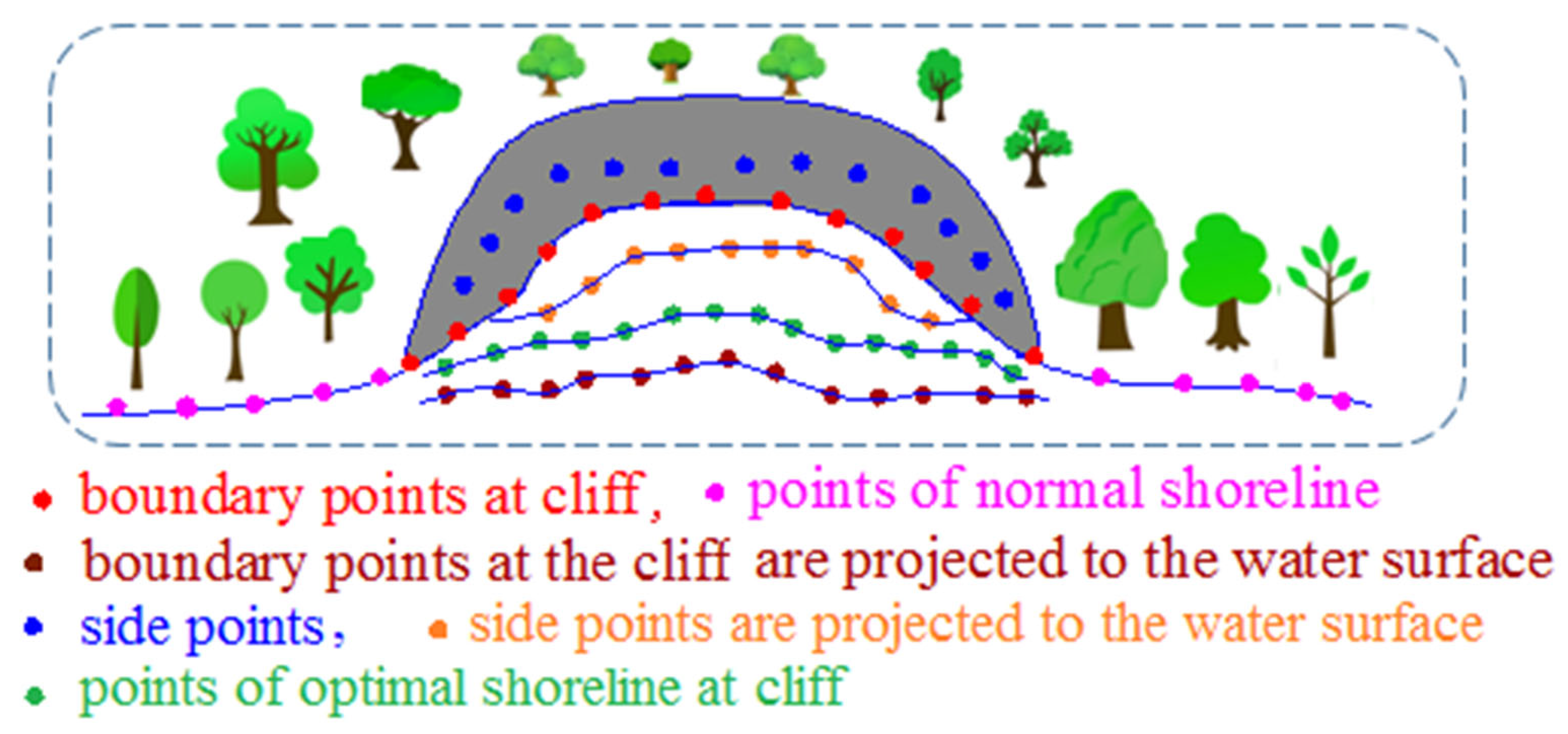
The elevation of points in the side point cloud is higher than that of the water surface; that is, points in the side point cloud calculated in Section 2.4 are above the water body. Therefore, while maintaining the x and y coordinates of as constant, the elevation coordinates of each point were corrected to ensure that each point is as close to the water surface as possible. Because there are two junction points A and B on the water surface, and the projected point should be close to the elevation of A and B, these points are selected as the start and end points of the elevation difference, respectively, the height difference weighted by distance of each point in is distributed, and points in are sorted according to the x coordinate from small to large, as shown in Figure 5.

Figure 5.
The schematic diagram of optimal estimation of coastline at cliff.
Of note, when calculating the distance here, the distance of the first point in is the distance between point A and the first point in , and the distance of the last point is the distance between the last point and B; then, the calculation formula is as follows:
where, is the elevation difference allocated to each point; is the distance between two adjacent points; N is the total number of points in ; and are the elevation of points A and B.
Assuming that the point cloud after projection and elevation correction is ,
2.6. Calculation of the Points of Optimal Coastline and Integration with the Points of Coastline Outside the Cliff
The points of the most inwardly inclined coastline were obtained from the projection and elevation correction of side points in Section 2.5; that is, when the specific terrain under the cliff is not clear, the most inwardly inclined coastline is the extreme coastline toward the land side, such that the coastline can no longer deviate toward the land side. Regarding the coastline of the cliff, if the edge of the cliff is almost vertical to the water surface, the collected edge point cloud is the coastline at the cliff, assuming that the coastline in this case is the outermost coastline. The outermost coastline can be obtained by projecting the boundary at the cliff section in Figure 3 onto the water surface, and correcting the elevation according to the elevations of points A and B. The median value between the innermost and outermost coastlines can be obtained by the design method, and this median value can be considered the optimal estimate of the coastline at the cliff. Specifically, the points of the innermost and outermost coastlines are sorted from small to large according to the x coordinate, and the two coastline points are converted into the same elevation surface and then separately connected into lines. Put the point cloud data of the innermost coastline and the outermost coastline into the same plane, and only consider their x and y coordinates. Considering the points of the innermost coastline as the standard, the vertical line of the x-axis passes through the x coordinate of each point and intersects the outermost coastline; this forms a straight line equation from the front and rear points of the outermost coastline and at the intersection, bringing in x coordinates to calculate the y coordinate of the intersection, mean value of y coordinates of points of the innermost coastline and the intersection, y coordinates of the middle point, and mean value of elevation. In this way, the three-dimensional coordinates of the intermediate points can be calculated, and the set of all these intermediate points constitutes the point cloud dataset of the optimal coastline, as shown in Figure 5. After calculating the point set of the optimal coastline, the point set of the coastline under the cliff is the point set of hollowed-out places under the cliff in this case. Therefore, the complete coastline of the coastal zone can be obtained by fusing the point cloud of this coastline with the point cloud of the coastline on both sides of the cliff. The fused point cloud dataset of the coastline is , and the point cloud completion method is used to interpolate. The completed point cloud dataset is . Combined with the average high-tide surface elevation determined by the hydrological observation data of local area, the point cloud of coastline in a strict sense is acquired.
3. Experiment and Analysis
3.1. Experiment on Coastline Extraction at the Cliff
This study used C++ programming language combined with PCL program to realize the algorithm described in Section 2.2, Section 2.3, Section 2.4, Section 2.5 and Section 2.6, extract the boundary of data in Figure 1a, and obtain the boundary point cloud , as shown in Figure 6a. According to Equation (1), the junction points of the flat and cliff areas were determined, and the coordinates of the two junction points A and B were calculated as follows: x = 516,101.62, y = 3,372,355.8, and z = 71.07001 for A, and x = 516,319.88, y = 3,372,341.2, and z = 71.11 for B. The boundary point cloud of this section at the cliff was extracted according to points A and B, as shown in Figure 6b. The boundary point cloud of the cliff section was projected onto the water surface, and the elevation of each point was corrected to obtain the outermost coastline point cloud at the cliff. Finally, the outermost coastline point cloud at the cliff was projected onto the water surface, on the premise of keeping the x and y coordinates unchanged. The elevation was corrected to make it approximately equal to the sea surface elevation, so as to obtain a new point cloud dataset.

Figure 6.
(a) Boundary point cloud dataset, ; (b) Boundary point cloud of cliff section.
Among the two junction points, A and B, the point closest to A in the x-direction and with the smallest elevation difference is point C, and the point closest to B in the x-direction, and with the smallest elevation difference is point D. The distance between A, B and C, D was calculated, and the average value of the two distances was determined to obtain the point cloud depth H of the cliff section. The calculated H value of these data was 217.532 m. Therefore, the boundary point cloud of the cliff section in Figure 6b was extracted as a point cloud with a depth value of H = 217.532 m. The point cloud obtained is shown in Figure 7a. Then, the x-coordinates of points A and B were used to intercept this point cloud in the given interval and obtain the point cloud at the cliff, as shown in Figure 7b.

Figure 7.
(a) Rough extraction of point cloud in cliff segment. (b) Extraction of point cloud in cliff segment in combination with the x coordinate interval of points A and B.
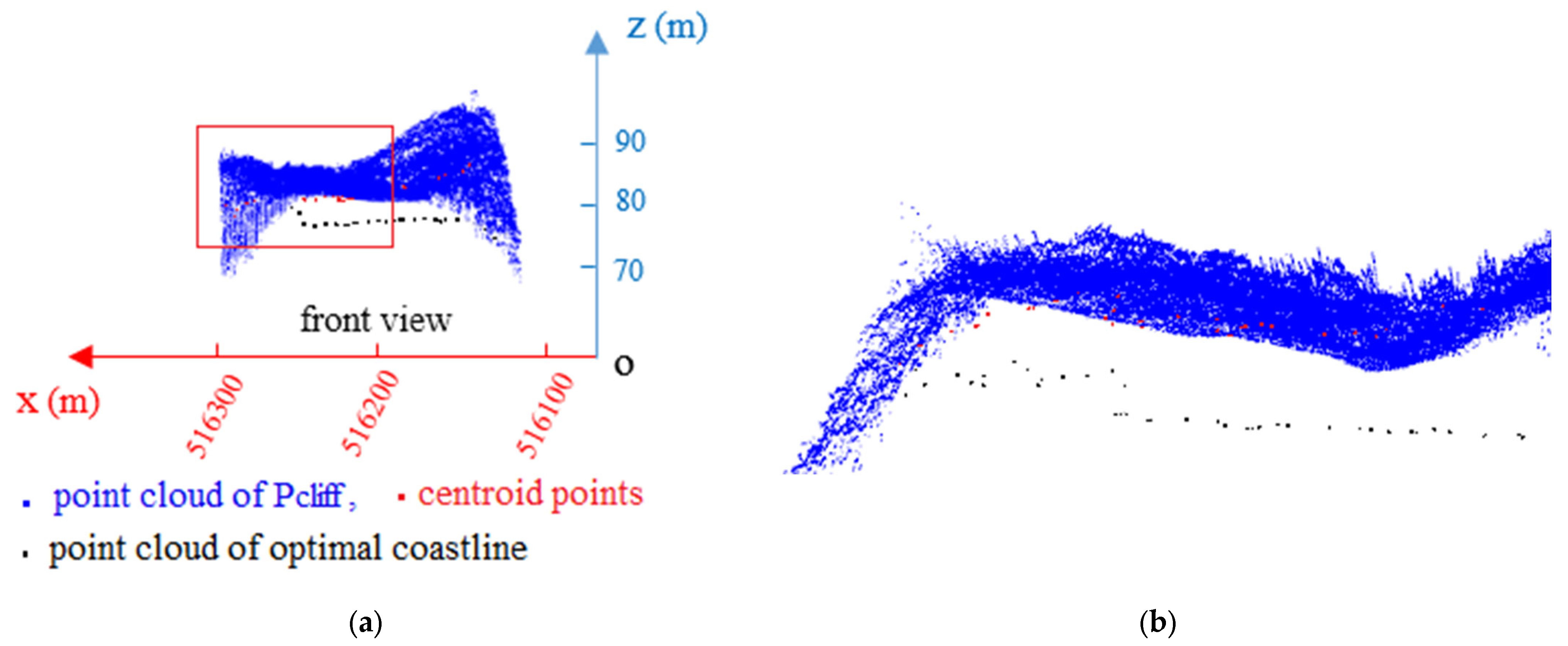
Points in were sorted according to the x-coordinate from small to large. Starting from the smallest x-coordinate, the cloud was divided into blocks at a certain interval. For our data, we set an interval of 5 m and set the minimum value of x as x_ min; that is, points whose x coordinates were between x_min and x_min + 5 formed a block, points with x coordinates between x_min + 5 and x_min + 10 formed another block, and so on. Thus, each point cloud was separated into five-unit blocks until the last point in . For each point cloud dataset, its centroid coordinates were calculated according to Equation (4), which were pooled into a point cloud dataset and displayed in-plane rectangular coordinate system, as shown in Figure 8a. The point clouds of the centroid and cliff segment points are shown in Figure 8b. Figure 8c shows an enlarged view of the red box in Figure 8b.
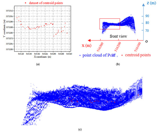
Figure 8.
(a) The point cloud of centroid. (b) Superposition display of point cloud of centroid and point cloud of cliff. (c) The enlarged view of the red box in Figure (b).
After obtaining the point cloud dataset of the centroid points, the coordinates of the side points of each block were calculated according to the centroid point coordinates and x-coordinates of the two boundaries of each block. The x-and y-coordinates of the side points were constant and projected onto the water surface. The elevation coordinates of each point were corrected according to the elevations of points A and B in the two sections, and the point cloud dataset of the side point projection coordinates was obtained. This point cloud dataset was recorded as , and its diagram is shown in Figure 9a. By combining the point cloud dataset of the outermost coastline at the cliff extracted at the beginning, the projection point cloud of side points, and the generation method of the optimal coastline, the point cloud of the optimal coastline was calculated, as shown in Figure 9b.
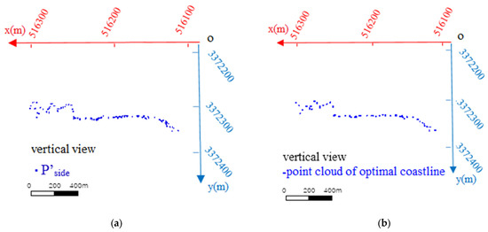
Figure 9.
(a) Projection point cloud of side points ; (b) Point cloud dataset of optimal coastline.
To reflect the relative positional relationship of the point clouds of the optimal coastline, centroid, and cliff, three-point cloud datasets were superimposed and are displayed in Figure 10a. The elevation of the optimal coastline points was closer to that of the water body, and their spatial height was closer to the water surface. Figure 10b shows an enlarged view of the red box in Figure 10a.
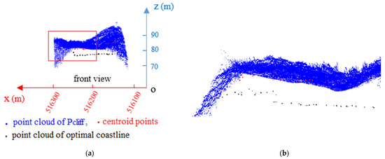
Figure 10.
(a) Superposition of point cloud of optimal coastline and centroid and point cloud at cliff; (b) The enlarged view of the red box in Figure (a).
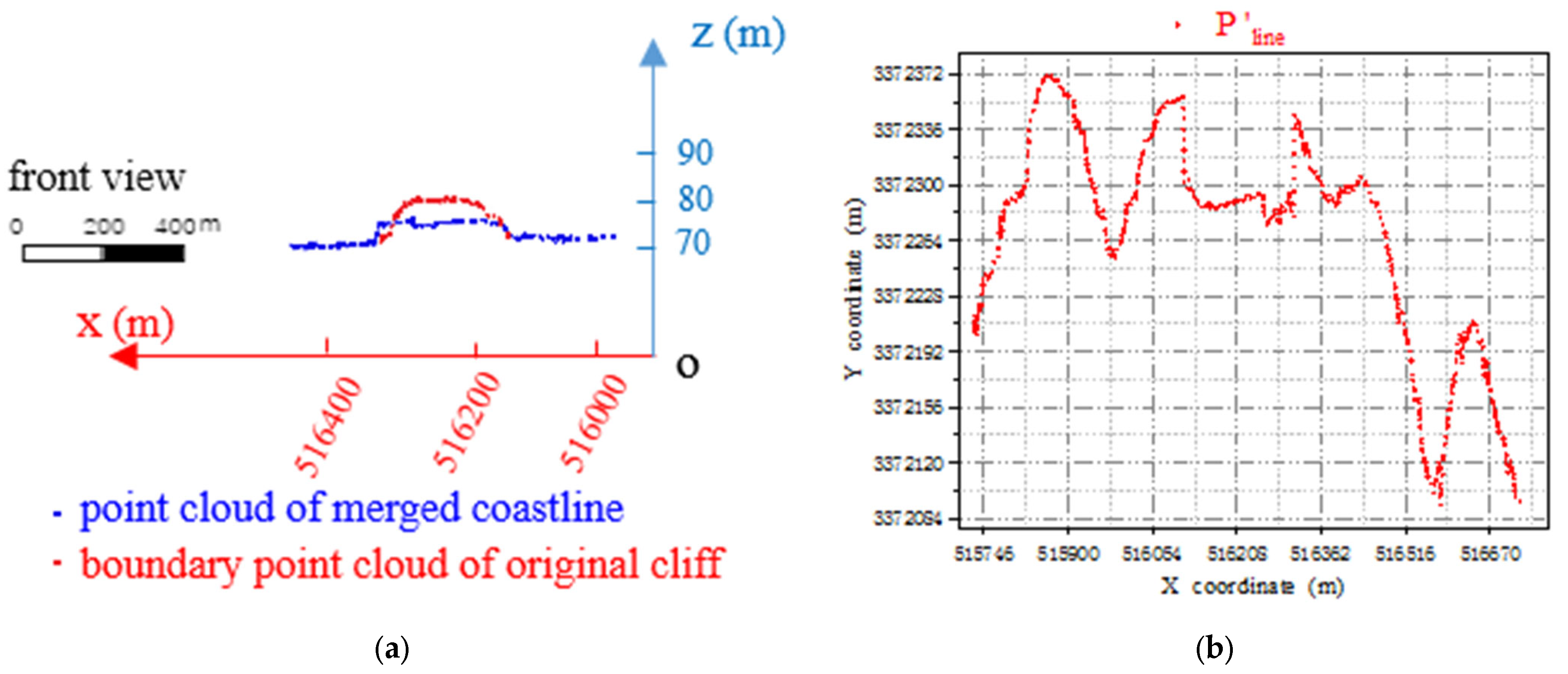
As the coastline of the cliff is only a small segment, it must be fused with the point cloud of the coastline outside the cliff. According to the boundary point cloud of data extracted in the previous step, the coastline of the entire sea area could be obtained by replacing the point cloud of the cliff segment with the point cloud of the optimal coastline. To depict the difference between the point cloud of the merged coastline and that of the original boundary, these datasets were superimposed and are displayed in Figure 11a. The red segment and arched point cloud in the figure represent the point cloud dataset of the original cliff-segment boundary. Since the water body has a plane-pushing property, the original cliff segment boundary cannot clearly represent the actual coastline. However, for the point cloud behind the red segment, the blue segment calculated from the data is closer to the actual coastline and can reflect the shape of the coastline more accurately. Subsequently, a point cloud completion method [5] was used to complete the appropriate points according to the distance between the two points. When the distance between two points is less than 0.5 m, two points are interpolated: when the distance is greater than 0.5 m and less than 1 m, four points are interpolated. When the distance is greater than 1 m and less than 2 m, six points are interpolated; when the distance is greater than 2 m, eight points are interpolated, and the coordinates of the interpolated points are calculated from the coordinates of the original two points according to the corresponding proportion. The point cloud of the integrated coastline was completed according to this method, and the point cloud was obtained, as shown in Figure 11b.

Figure 11.
(a) Superposition of point cloud of coastline after fusion and original boundary point cloud; (b) The completion of point cloud of coastline after fusion.
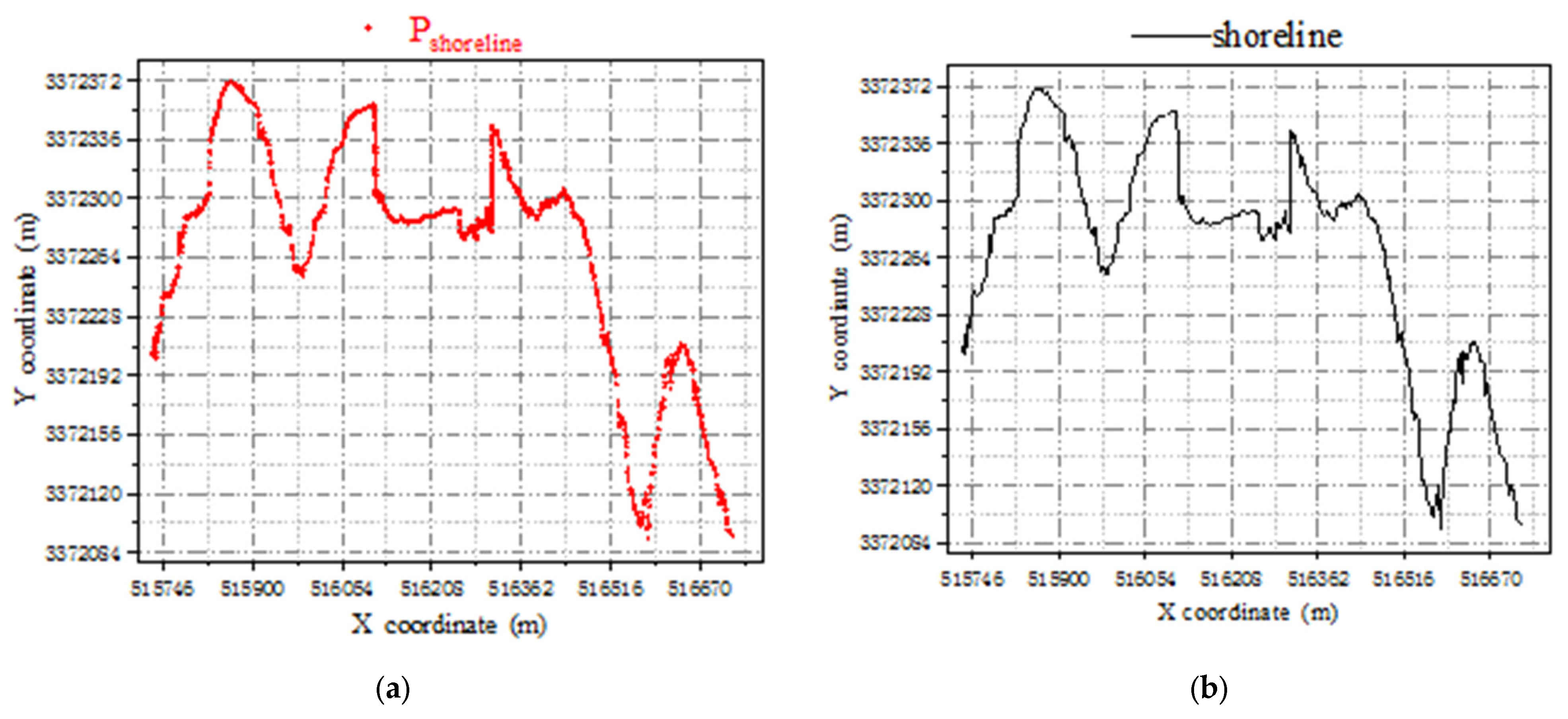
Based on the average high-tide surface elevation determined by the hydrological observation data of Longkou City, Shandong Province, the point cloud of the coastline in a strict sense was extracted and recorded as . Then, the points in were supplemented to obtain the point cloud , as shown in Figure 12a. Points in were sorted from small to large according to their x-coordinates and connected to obtain the coastline trend, as shown in Figure 12b.

Figure 12.
(a) Point cloud dataset, ; (b) The coastline generated by .
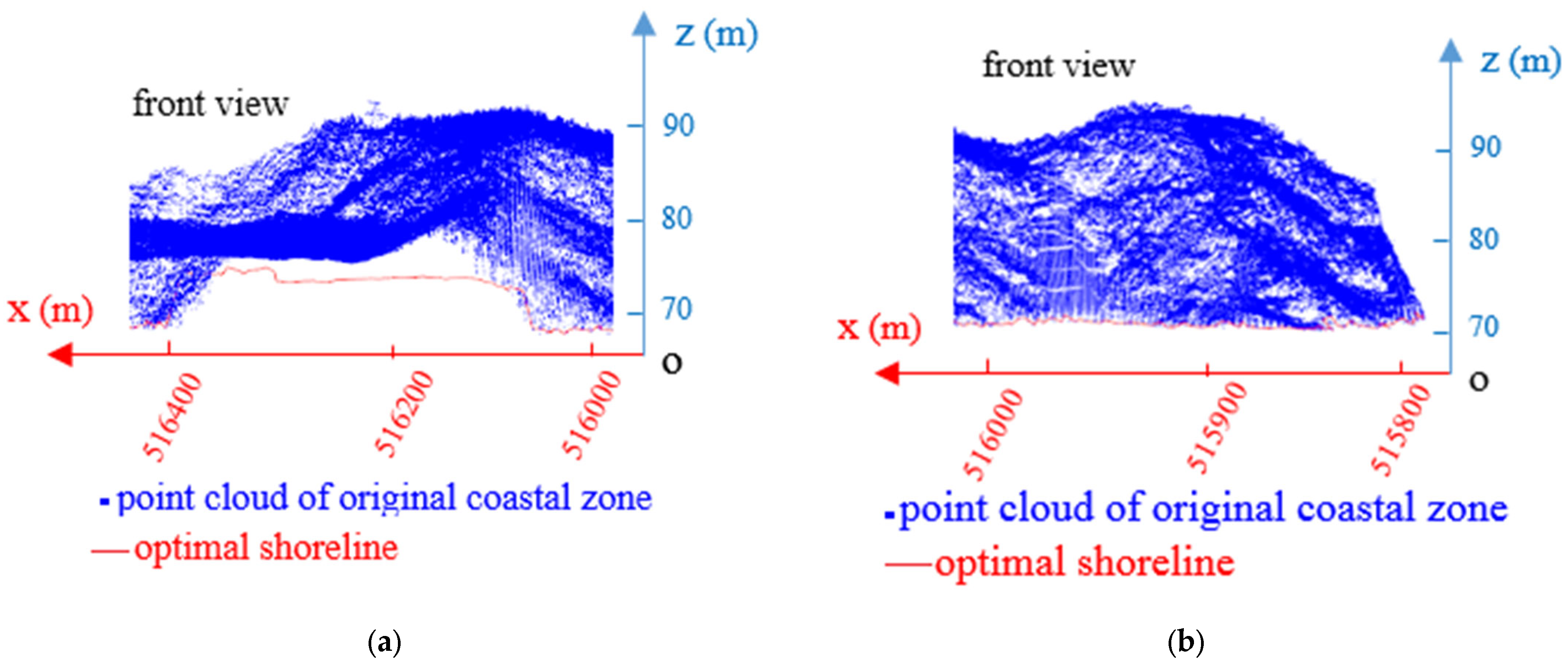
A superimposed display of the point cloud of the fused coastline and the corresponding point cloud of the coastal zone is presented in Figure 13.
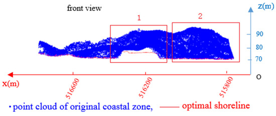
Figure 13.
The superimposed display of the point cloud of integrated coastline and coastal zone.
To analyze the generated coastline in greater detail, Areas 1 and 2 in Figure 13 are enlarged and displayed in Figure 14a,b, respectively.
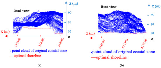
Figure 14.
(a) The enlarged view of block 1; (b) The enlarged view of block 2.
3.2. Comparison with Other Methods
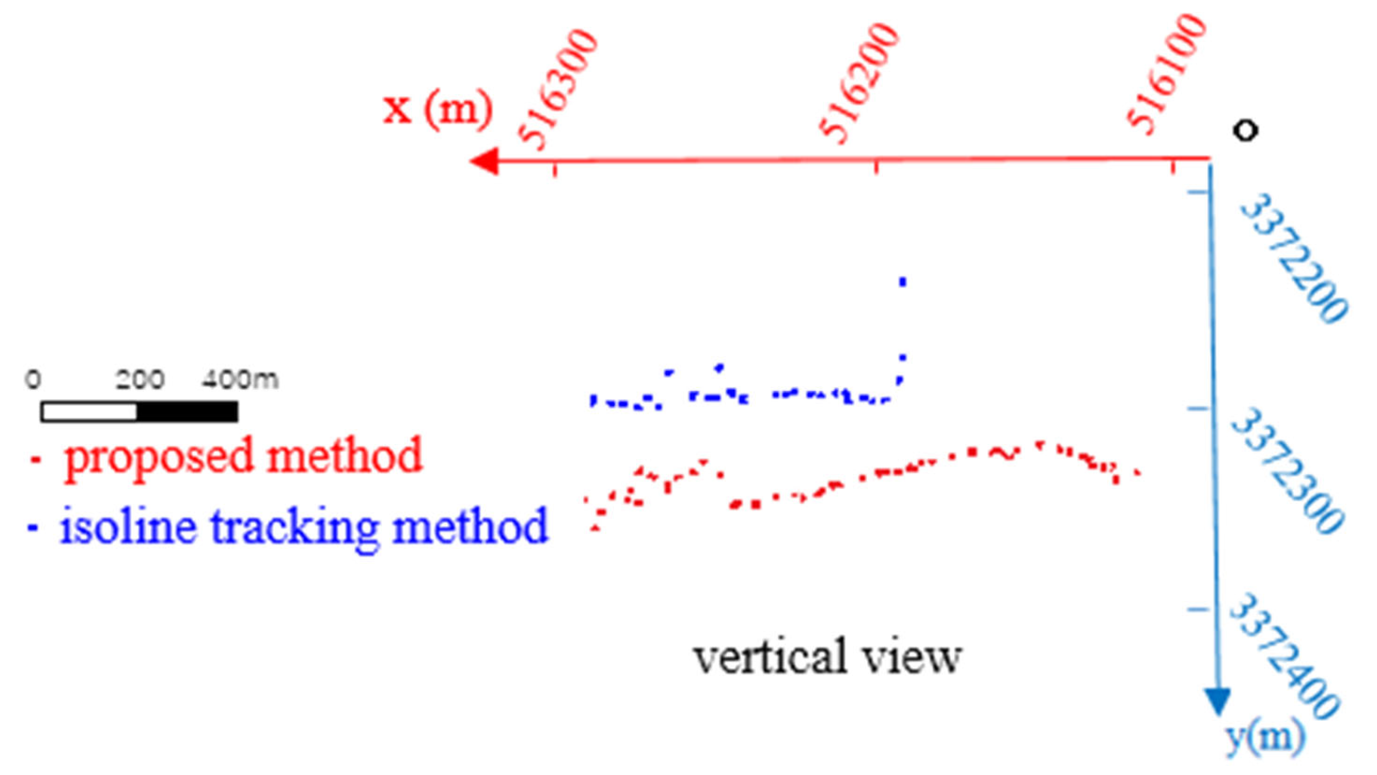
Common coastline extraction methods based on LiDAR data include the coastal profile and isoline tracking methods. In the coastal profile method, a DEM is first constructed using LiDAR data; it is then divided into many profiles with different elevations, and finally a profile in which the coast is located is identified. In the isoline tracking method, a DEM is first built using the LiDAR data and then the isoline at which the average high-tide surface elevation is located is identified; this isoline is known as the coastline. However, the coastline extracted by the coastal profile method has large errors and discontinuities; therefore, the isoline tracking method is considered superior to the coastal profile method. In this context, the present study selected and compared the performance of our proposed method with that of the isoline tracking method. Since the present study mainly focused on the extraction of the coastline at the cliff, the object of comparison was the coastline of the cliff section. The contour tracing method identifies the contour corresponding to the elevation of the average high-tide surface of the spring tide in DEM; however, according to the elevation characteristics of points in the cliff section, all points close to the elevation of the average high-tide surface of the spring tide are in the lower part of the cliff toward the land; thus, the extracted points will be far away from the outermost edge of the cliff. The isoline point cloud obtained using the extraction principle of the isoline tracking method is shown in Figure 15. The superimposed display of the coastline point cloud extracted using the proposed method and that generated using the isoline tracking method is also presented in Figure 15. As shown in Figure 15, the elevation of several blue points, that is, points generated by the isoline tracking method, abruptly increases, indicating a large jitter here, which is an anomaly. And there are large gaps in some areas behind, indicating that the points here are discontinuous. Compared with the red points, that is, points generated in the present study using the proposed method, the height change is relatively gentle and the points are not evenly divided, indicating excellent continuity.
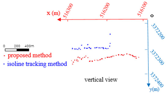
Figure 15.
The superposition of this method and isoline tracking method.
The superimposed display of the coastline point clouds calculated using the proposed method and the isoline tracking method and the point cloud of the cliff segment are presented in Figure 16a. Points in the red box, that is, green points, were calculated with the isoline-tracking method. In the figure, the green points will be projected into the water surface, so the red and green points are approximately in the same plane, and their elevations are close. Figure 16b shows the superposed display of coastlines generated based on the two types of points and point clouds of the cliff section. The green coastline shows a large error and a large deviation from the actual trend, whereas the red coastline is smoother, continuous, and closer to reality.
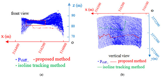
Figure 16.
(a) The superposition of point cloud of the two methods, and point cloud of cliff segment; (b) The superposition of coastline of the two methods, and point cloud of cliff segment.
According to error theory, when the true value is unknown and there are multiple groups of observations, the average value of each group of observations can be regarded as its approximate true value. Therefore, assuming that the coastlines generated by the proposed method and the isoline tracking method are correct, the position of the average coastline can be calculated from these two groups of observations. Specifically, the two coastlines are converted to the same elevation plane; that is, they are in the same plane, and only the accuracy of their x- and y-coordinates is assessed. For the adjacent straight lines perpendicular to the x-axis, the difference in x values was fixed and small, which was set to 0.05 m in this case. These lines perpendicular to the x-axis intersect both shorelines, and the y-coordinate of the intersection can be inversely calculated according to the straight line composed of two points before and after the intersection. The y coordinate of the average shoreline is the average value of y coordinates calculated by the two types of shorelines, and the coordinate points of the average shoreline can then be calculated. Considering the points of the average coastline as the standard and passing a parallel line of the y-axis through the x coordinate of each point, the parallel line intersects the coastline extracted by the proposed method and the isoline tracking method. The accuracy of the two methods was estimated according to the accuracy estimation method [5], which is to calculate the x, y standard deviation and variance of the whole coastline by calculating the difference between each point and the average value; the data is shown in Table 1. Error range refers to the interval segment of the y coordinate error value, and error range (points) refers to the number of points where the y coordinate error value is in this error interval. It can be seen from the table that the variance and standard deviation of the shoreline extracted by this method are 0.1528 and 0.0233, and the variance and standard deviation of the isoline tracking method are 0.3638 and 0.1338. Therefore, the shoreline extracted by this method has less error and higher accuracy.

Table 1.
The error and accuracy data of the two methods.
4. Conclusions
In this study, a method was designed to extract the coastline of a cliff area using stress analysis of the cliff section and the calculation criterion of point cloud segmentation. Our experiment, using typical sea area data, proved that the proposed method could effectively extract the coastline. We further compared the proposed method with the isoline tracking method. Notably, the coastline extracted by the isoline tracking method was inconsistent with the actual situation, whereas the coastline extracted using the proposed method was more consistent with the actual trend, as evidenced by the smoother and more continuous coastline. The proposed method can be applied to estimate coastlines sheltered under solid or large hollowed-out cliffs, as well as coastlines of tall rock coasts closely connected to a water area. Our method compensates for the lack of a coastline extraction method at the cliff, enabling the extraction of complete coastlines to solve the problem of missing data in relevant research. Moreover, our results can serve as a reference to develop other methods for the extraction of coastlines in cliff areas.
Author Contributions
C.Q. is mainly responsible for the collection of experimental data and the testing of code, H.L. is mainly responsible for the testing of code and the experiment of each data, and W.L. is mainly responsible for the design, implementation, testing of the algorithms and writing this document. All authors have read and agreed to the published version of the manuscript.
Funding
This work was supported by the National Natural Science Foundation of China (41771482), the Natural Science Research Project of Jinggangshan University (JZ2002).
Data Availability Statement
All data, models, or code generated or used during the study are available from the corresponding author by request.
Acknowledgments
Thank Wu for providing valuable suggestions.
Conflicts of Interest
The authors declare no conflict of interest.
References
- Stockdonf, H.F.; Sallenger, A.H., Jr.; List, J.H.; Holman, R.A. Estimation of Shoreline Position and Change Using Airborne Topographic Lidar Data. J. Coast. Res. Summer 2002, 18, 502–513. [Google Scholar]
- Robertson, W.; Whitman, D.; Zhang, K.; Leatherman, S.P. Mapping Shoreline Position Using Airborne Laser Altimetry. J. Coast. Res. 2004, 203, 884–892. [Google Scholar] [CrossRef]
- Xu, S.; Ye, N.; Xu, S. A new method for shoreline extraction from airborne LiDAR point clouds. Remote Sens. Lett. 2019, 10, 496–505. [Google Scholar] [CrossRef]
- Luque, I.F.; Torres, F.J.A.; Torres, M.A.; García, J.L.P.; Arenas, A.L. A New, Robust, and Accurate Method to Extract Tide-Coordinated Shorelines from Coastal Elevation Models. J. Coast. Res. 2012, 28, 683–699. [Google Scholar] [CrossRef]
- Li, W.; Liu, H.; Qin, C. A method for the extraction of shorelines from airborne lidar data in muddy areas and areas with shoals. Remote Sens. Lett. 2022, 13, 480–491. [Google Scholar] [CrossRef]
- Liu, H.; Sherman, D.; Gu, S. Automated Extraction of Shorelines from Airborne Light Detection and Ranging Data and Accuracy Assessment Based on Monte Carlo Simulation. J. Coast. Res. 2007, 236, 1359–1369. [Google Scholar] [CrossRef]
- Incekara, A.H.; Seker, D.Z.; Bayram, B. Qualifying the LIDAR-Derived Intensity Image as an Infrared Band in NDWI-Based Shoreline Extraction. IEEE J. Sel. Top. Appl. Earth Obs. Remote Sens. 2018, 11, 5053–5062. [Google Scholar] [CrossRef]
- Wei, L.; Yang, B.; Jiang, J.; Cao, G. Adaptive algorithm for classifying LiDAR data into water and land points by multi-feature statistics. J. Appl. Remote Sens. 2016, 10, 045020. [Google Scholar] [CrossRef]
- Smeeckaert, J.; Mallet, C.; David, N.; Chehata, N.; Ferraz, A. Large-scale classification of water areas using airborne topographic lidar data. Remote Sens. Environ. 2013, 138, 134–148. [Google Scholar] [CrossRef]
- Yousef, A.; Iftekharuddin, K.M.; Karim, M.A. Shoreline extraction from light detection and ranging digital elevation model data and aerial images. Opt. Eng. 2013, 53, 011006. [Google Scholar] [CrossRef]
- Demir, N.; Bayram, B.; Şeker, D.Z.; Oy, S.; İnce, A.; Bozkurt, S. Advanced Lake Shoreline Extraction Approach by Integration of SAR Image and LIDAR Data. Mar. Geod. 2019, 42, 166–185. [Google Scholar] [CrossRef]
- Sukcharoenpong, A.; Yilmaz, A.; Li, R. An Integrated Active Contour Approach to Shoreline Mapping Using HSI and DEM. IEEE Trans. Geosci. Remote Sens. 2015, 54, 1586–1597. [Google Scholar] [CrossRef]
- Yang, B.; Hwang, C.; Cordell, H.K. Use of LiDAR shoreline extraction for analyzing revetment rock beach protection: A case study of Jekyll Island State Park, USA. Ocean. Coast. Manag. 2012, 69, 1–15. [Google Scholar] [CrossRef]
- Yun, M.; Choi, C. Spatial analysis of Shoreline change in Northwest coast of Taean Peninsula. Korean J. Remote Sens. 2015, 31, 29–38. [Google Scholar] [CrossRef][Green Version]
- Lee, I.S.; Park, H.J.; Lee, J.O.; Kim, Y.S. Delineating the Natural Features of a Cadastral Shoreline in South Korea Using Airborne Laser Scanning. IEEE J. Sel. Top. Appl. Earth Obs. Remote Sens. 2011, 4, 905–910. [Google Scholar] [CrossRef]
- Nassif, F.B.; Pimenta, F.M.; D’Aquino, C.D.A.; Assireu, A.T.; Garbossa, L.H.P.; Passos, J.C. Coastal Wind Measurements and Power Assessment. Using a LIDAR on a Pier. Rev. Bras. De Meteorol. 2020, 35, 255–268. [Google Scholar] [CrossRef]
- Yu, C.; Xu, J.; Xu, J.; Zheng, Y.; Li, G. A new method for extracting coastline from LiDAR point cloud. Surv. Mapp. Bull. 2015, 10, 66–68. [Google Scholar] [CrossRef]
- Jiang, H.; Huang, J.; Yu, Y.; Fan, Y.; Dong, G. Coastline extraction method under multiple constraints of coarse and fine grids. J. Surv. Mapp. Sci. Technol. 2020, 37, 392–397. [Google Scholar]
- Yu, C.; Wang, J.; Feng, J.; Xu, J.; Chen, H. A coastline extraction method based on LiDAR point cloud grid. J. Surv. Mapp. Sci. Technol. 2015, 32, 187–191+196. [Google Scholar]
- Bengoufa, S.; Niculescu, S.; Mihoubi, M.K.; Belkessa, R.; Abbad, K. Rocky Shoreline Extraction Using A Deep Learning Model And Object-Based Image Analysis. Int. Arch. Photogramm. Remote Sens. Spat. Inf. Sci. 2021, XLIII-B3-2021, 23–29. [Google Scholar] [CrossRef]
- Sun, W.; Ma, Y.; Zhang, J.; Liu, S.; Ren, G. Study of Remote Sensing Interpretation Keys and Extraction Technique of Different types of Shoreline. Bull. Surv. Mapp. 2011, 3, 41–44. [Google Scholar]
Publisher’s Note: MDPI stays neutral with regard to jurisdictional claims in published maps and institutional affiliations. |
© 2022 by the authors. Licensee MDPI, Basel, Switzerland. This article is an open access article distributed under the terms and conditions of the Creative Commons Attribution (CC BY) license (https://creativecommons.org/licenses/by/4.0/).


