Article

Topology Optimization Based Material Design for 3D Domains Using MATLAB

by
George Kazakis
and
Nikos D. Lagaros
*,†
Institute of Structural Analysis and Antiseismic Research, School of Civil Engineering, National Technical University of Athens, 9, Heroon Polytechniou Str., Zografou Campus, GR-15780 Athens, Greece
*
Author to whom correspondence should be addressed.
These authors contributed equally to this work.
Appl. Sci. 2022, 12(21), 10902; https://doi.org/10.3390/app122110902
Submission received: 28 September 2022 / Revised: 14 October 2022 / Accepted: 24 October 2022 / Published: 27 October 2022
(This article belongs to the Section Additive Manufacturing Technologies)

Abstract

:
In this work, a simple, easy to use MATLAB code is presented for the optimal design of materials for 3D domains. For the optimal design of materials, the theoretical framework of topology optimization and that of homogenization were utilized to develop a formulation where the design of the micro-structure of the material is affected among others by the loading and boundary conditions of the 3D macro domain. The final result of the micro-scale can then be converted into an stl file, which can be utilized for 3D printing; however, the continuity of the unit cells when assembled to form the macro structure should be taken into account. The transition of the design of the material problem formulation from 2D to 3D domains generates drastically increased computational needs in order to perform the design procedures, which might narrow its formulation scales and the corresponding sizes of the adopted finite element discretization. Thus, in addition to the optimal design of materials implementation, the utilization of three different model order reduction (MOR) approaches is presented, aiming to assist towards the reduction of the computational cost of the two scales formulation. On-the-fly reduced order model, proper orthogonal decomposition (POD), and approximate reanalysis (AR) following the combined approximations are the three approaches adopted for the purposes of this study, while the code implementation enables the addition of new ones easily.

1. Introduction

The main focus of this work is to present a compact and easy-to-use MATLAB code for 3D material design based on the topology optimization formulation and the homogenization theory. The MATLAB programming language was chosen based on the existing codes published in MATLAB, covering most of the required different parts. Since the first MATLAB Structural Topology Optimization (STO) code t o p 99 , which was published by Sigmund [1], many others have been published, concerning different aspects of the topology optimization procedure. Most notably, after the release of the t o p 99 , an improved version labelled as t o p 88 was published by Andreassen et al. [2], where the advanced features of the matrix manipulation capabilities of MATLAB were utilized, aiming to reduce the computational cost of the entire procedure. Based on the t o p 88 MATLAB code, its extension to 3D domains was published by Liu and Tovar [3] and later a modified version developed by Ferrari and Simgund [4] was presented. All these code implementations were based on the SIMP approach of the topology optimization formulation. Subsequently, Huang and Xie [5] published a MATLAB code that was based on the t o p 99 code, which implemented the BESO approach in the topology optimization formulation; whereas Challis [6], also based on the t o p 99 code, published a script implementing the level set based approach. In the scope of the level set based topology optimization approach, additional MATLAB codes have been published, e.g., by Wang et al. [7], by Otomori et al. [8], where the reaction diffusion equation was utilized instead of the Hamilton–Jacobi equation, and by Wei et al. [9], where radial basis functions were used to smoothen the level set function. Talishi et al. [10] published P o l y T o p , utilizing unstructured mesh generation techniques in conjunction with the power-law approaches for 2D domains, while Chi et al. [11] expanded this formulation to 3D domains through P o l y T o p 3 D .
As far as concerns the homogenization theory, two MATLAB codes have been published dealing with the theory of homogenization, covering both 2D and 3D domains. In particular, Andreassen and Andreasen [12] published a MATLAB code computing the homogenized elasticity matrix for the case of 2D domains and Dong et al. [13] expanded this formulation for cases of 3D domains, computing the homogenized elasticity tensor. Based on the theory of homogenization and utilizing the t o p 88 MATLAB code Xia and Breitkopf published a code for the design of materials using the theory of topology optimization and energy-based homogenization. Gao et al. later published two codes [14] that perform a concurrent topology optimization formulation, i.e., optimization was performed both on the micro and macro scales. These codes also rely on the t o p 88 MATLAB code and are utilizing the energy-based homogenization method. Aiming to improve the computational efficiency for both 2D and 3D formulations of the topology optimization, Amir et al., in Refs. [15,16], published a MATLAB implementation of the multigrid preconditioned conjugate gradient (MGCG) applied onto a topology optimization. In addition, Kazakis and Lagaros recently published [17] a MATLAB implementation for the material design utilizing the theory of homogenization using its asymptotic approach and combining the computational efficiency of model order reduction (MOR) techniques for the case of 2D design domains. In this work, an extension of the recently published [17] work of the authors to 3D domains is presented, adding new features for efficient implementations of the MOR techniques, which are capable of being applied on both macro and micro scales.
The layout of this study is composed of four sections, as well as Introduction and Conclusions sections. In further detail, the theoretical framework of material design using topology optimization and homogenization can be found in Section 2. Next, a compact description of the three MOR models implemented in the final formulation is presented in Section 3, followed by a detailed description of the MATLAB code implementation in Section 4, while a detailed description for implementing the code in three test examples can be found in Section 5. Topology optimization is directly linked with additive manufacturing [18,19]. Thus, in the test examples in Section 5, some of the resulting optimized topologies on the micro scale are converted into a STL format. The MATLAB code files presented in this study are listed in here.

2. Design of Materials by Means of STO

For the needs of the optimal material design problem formulation, two different scales are utilized during the optimization procedure. The first one refers to the macro scale, where the structural domain is defined where the loads are applied, while the second one concerns the micro scale where the design domain (unit cell) is formulated. Compared to the classical STO problem formulation and in order to apply the topology optimization approach for the optimal design of materials, the main modification required concerns the design variables (material densities). More specifically, instead of assigning the unknown material densities x on every finite element of the macro domain discretization, unknowns x are assigned on each finite element of the micro design domain. The bridging between the two scales is implemented by means of the homogenization theory. The mathematical expression of the optimal design of materials problem is represented by the formulation of Equation (1) (Throughout the text, a common notation for all cases of the multiplication operators is used consistently and its correct interpretation depends on the context of the algebraic objects appearing on the left and right sides of the “·” sign), which does not differ at the first site with the formulation of the classical problem. As denoted, earlier the difference is hidden in the two scales adopted by the material design problem (micro and macro ones).
C ( x ) = F T · U ( x ) s . t . F = K · U ( x ) V ( x ) / V 0 = f 0 x e 1
where the structural compliance value C ( x ) is the objective function to be minimised, vector F contains the loading conditions applied to the macro domain, U ( x ) is the resulting displacements vector obtained through the solution of the F = K · U ( x ) that refers to the structural equilibrium system of equations that is defined for the macro domain, V ( x ) and V 0 denote the structural volume and the domain volume, respectively. The volume target percentage is denoted with f and x e , which are the material density of element e at the micro design domain level (also called unit cell). As denoted earlier, it can be observed that the formulation of Equation (1) is almost the same as that of the classical STO problem with the alteration on the scale where the material densities are applied. In order to solve the formulation presented by the expression of Equation (1), the derivative of the objective function (compliance) is needed. Taking advantage of the calculations used by the classical topology optimization theoretical framework, the derivative of the compliance with respect to the material densities C / x e is computed from the following expression of Equation (2):
C x e = U e T · K e x e · U e
where U e ( e = 1 , , N e ) are the displacement vectors of every finite element e of the macro domain ( N e is the total number of elements used to discretize the macro domain), K e / x e is the derivative of the macro domain element’s e stiffness matrix K e with respect to the material densities assigned to finite elements of the micro design domain. The displacement vector U e is obtained as the outcome of the solution of the equilibrium equation presented by Equation (1), expressed at the macro domain, whereas the derivative of the element stiffness matrix is computed from the following expression of Equation (3):
K e x e = C H x e · K e 0
where C e H / x e is the derivative of the homogenized elasticity tensor with respect to the material densities and K e 0 is the element stiffness matrix without using the elasticity tensor for its calculation. To obtain the homogenized elasticity tensor, the theory of homogenization is utilized. According to the homogenization theory, the homogenized elasticity tensor C H for a non-homogeneous material is obtained by applying two sets of unit strains onto the material unit cell. The first set of unit strain is applied at the unit cell as a whole, whereas the second one is applied at each finite element of the unit cell. Utilizing the resulting displacement field, the homogenized elasticity tensor C H is computed from the following expression of Equation (4):
C i , j H = 1 V e = 1 n e x e ( u e 0 ( i ) u e ( i ) ) · k e · ( u e 0 ( j ) u e ( J ) ) d V e
where V refers to the unit cell volume, n e refers to the number of finite elements used to discretize the unit cell (micro design domain), u e 0 refers to the displacement field resulting from the unit strains applied to the unit cell as a whole, u e refers to the displacement field resulting from the unit strains applied to each finite element and k e refers to the element stiffness matrix of each finite element used to discretize the unit cell. The derivative of the homogenized elasticity tensor with respect to the material densities C e H / x e is computed using the following expression from Equation (5):
C H x e = E x e · 1 V x e ( u e 0 ( i ) u e ( i ) ) · k e 0 · ( u e 0 ( j ) u e ( J ) ) d V e
where E / x e refers the derivative of the element Young’s modulus with respect to the material densities and k e 0 refers to the original element stiffness matrix. To obtain the derivative of the element Young’s modulus with respect to the material densities the modified SIMP approach is utilized [20]. Thus, Young’s modulus E ( x ) is computed through the modified SIMP approach using the following expression of Equation (6):
E ( x ) = E m i n + x p · ( E 0 E m i n )
where E m i n is a very small value of Young’s modulus, used to avoid elements with Young’s modulus equal to zero for the cases where material density x e = 0 of element e is equal to zero, x is the vector of the material densities assigned to the finite elements, p is the penalization factor, and E 0 is the original elements’ Young’s modulus. Thus, the derivative of Young’s modulus with respect to the material densities is obtained using the following expression of Equation (7):
E x e = p · x p 1 · ( E 0 E m i n )
Based on the procedure described above, the derivative of the compliance with respect to the material densities of the unit cell can be obtained. By modifying the calculation process of the derivative for the compliance, the rest of the optimization procedure remains relatively the same to the one of the classical STO formulation.

3. Model Order Reduction in Material Design Optimization

The main objective of model order reduction (MOR) techniques is to reduce the dimensionality of a linear system of equations, which is solved multiple times. In the case of structural optimization procedure (STO) problems, including when the equilibrium equations system is solved multiple times, the use of such techniques can produce significant computational benefits for the entire process. In this part of the study, three MOR techniques are presented. We focus on their application to the material design optimization problem provided by the STO problem formulation. Although in this study three MOR techniques are integrated in the subsequently presented Matlab code, the code can easily be extended with the addition of new ones, i.e., the Proper Orthogonal Decomposition (POD), On-the-fly Reduced Order Model Construction, and the Approximate Reanalysis. These techniques have also been described in the work of the authors [17]; thus, their description will be presented very briefly herein.
Among the three MOR techniques, the main difference is the construction of the reduced basis matrix Φ , which contains the reduced basis vectors. This matrix is utilized by the MOR to reduce the dimensionality of the equilibrium system of the equations. Thus, instead of solving the equilibrium system of the equations, a system with smaller size is solved following the expression of Equation (8):
F = K · U F e f f K e f f · y
where y is a reduced approximation of the displacement field and F e f f and K e f f are computed following the expressions of Equations (9) and (10), respectively:
F e f f = Φ · F
and
K e f f = Φ T · K · Φ
The dimensions of the reduced basis matrix Φ are N b × d o f s . N b is the number of the reduced basis vectors and dofs are the number of degrees of freedom for the system of equilibrium equations. To assess the accuracy of the resulting displacement field, the following expression of Equation (11) can be used:
e 2 = K · Φ · y F 2 F 2
In this expression, the approximate solution Φ · y is utilized to compute the residual force resulting from the use of MOR. If the residual force increases, then the MOR reduces the basis matrix Φ , which needs to be updated to continue obtaining results of acceptable accuracy. In the case of STO problem formulations due to the use of the approximate solution Φ · y in the sensitivities calculation part, an additional term can be used to the expression of Equation (2) to account for the inaccuracy of the approximation, as provided in the following expression of Equation (12):
C x e = U e T · K e x e · U e = y T · Φ T · K x e · Φ · y i = 1 N b λ i T · K i x e · U i
where λ i is computed using the following expression of Equation (13) for each reduced basis N b .
K i · λ i = 2 · y i · ( F K · Φ · y i )
where K i refers to the stiffness matrix corresponding to the reduced basis i, y i refers to the reduced displacement field of the reduced basis i and K, Φ , and y refer to the current stiffness matrix, the reduced basis matrix, and the current reduced displacement field, respectively. In the following sections the construction of the reduced basis matrix for the three MOR techniques are presented.

3.1. Proper Orthogonal Decomposition

Aiming to create the reduced basis matrix Φ , the POD technique utilizes the singular value decomposition (SVD) factorization method. According to the SVD factorization method, a matrix is decomposed into three parts, as depicted in the following expression of Equation (14):
A = U ¯ · Σ · V
For a detailed explanation of the SVD factorization technique, the reader can refer to [21]. Among the three matrices generated by means of the SVD method, matrix U ¯ is used as the reduced basis Φ for the case of the POD technique. Matrix A is created using the resulting displacement field based on information collected through a small number of initial optimization iterations performed using the full system of equilibrium equations. Thus, according to POD, a small number of initial full dimensionality iterations are performed. The resulting displacement fields are used to formulate matrix A and SVD is applied to create the reduced basis matrix Φ . If during the optimization the residual force increases significantly, then a new full dimensionality iteration is performed. Matrix A is then updated using the new displacement field resulting from the new iteration, removing the oldest displacement field, and SVD operates to create the updated reduced basis matrix  Φ .

3.2. On-the-Fly Reduced Order Model Construction

Similarly to the POD technique, according to the on-the-fly technique, the reduced basis matrix is constructed by utilizing the displacement fields resulting from the initial small number of performed full dimensionality iterations, and then a Gram–Schmidt orthogonalization step is used. Thus, the first column of the reduced basis matrix Φ is created with the following expression of Equation (15):
Φ 1 = U 1 U 1
where the reduced basis vector Φ 1 is created from a normalization of the first displacement field vector. The rest of the columns are generated following the expressions of Equations (16) and (17):
Φ ^ i + 1 = U i + 1 j = 1 i U i + 1 , Φ j Φ j
Φ i + 1 = Φ ^ i + 1 Φ ^ i + 1
where a Gram–Schmidt orthogonalization procedure is applied by taking into account all previous reduced basis vectors and then a normalization step is performed to create the rest of the reduced basis vectors Φ i . The integration of the on-the-fly technique into the STO procedure is very similar to that of the POD one, differing only on the creation and updated steps of the reduced basis matrix Φ .

3.3. Approximate Reanalysis

In the case of the approximate reanalysis, the reduced basis matrix Φ is created at every iteration from scratch. Only the first reduced basis vector Φ 1 and the corresponding stiffness matrix are preserved throughout all iterations of the STO procedure. Thus, the first column of the reduced basis matrix Φ (first reduced basis vector) is computed following the expression of Equation (18), and the stiffness matrix K 0 is saved.
Φ 1 = U 1 = K 0 1 · F
Then in every iteration utilizing the reduced basis vector Φ 1 and the stiffness matrix K 0 , the reduced basis matrix Φ is created from the following expression of Equation (19):
Φ i = K 0 1 · ( F Δ K · Φ i 1 ) i = 2 i m a x
where Δ K denotes the difference between matrix K 0 and the stiffness matrix of the current iteration; i m a x denotes the maximum number of reduced basis vectors to be created. It is worth noticing that the inverse of matrix K 0 is computed once at the first iteration of the process and is then used in (19) without the need to be computed again. The reduced basis matrix Φ is constructed in every iteration, while it is defined using Equation (19). In addition, the first reduced basis vector Φ 1 needs to be updated during the optimization procedure. Similarly to the other two techniques, the time for updating the reduced basis matrix is controlled by the value of the residual force but can also be set to be performed after a fixed number of STO problem solution iterations or by taking into account the change of the objective function and the design variables. A more detailed review of the approximate reanalysis approach can be found in Ref. [22].

4. The MATLAB Code Implementation

In this section, the methodologies described in previous sections are presented using a MATLAB implementation for the case of 3D domains (for the micro and macro scales). The implementation is in accordance to that of the work of the authors [17], who extended into the 3D domain, including additional features required for the 3D design space and the two scales (micro and macro). The main function of the 3D material design is called UCOpt3D, and it is based on the top3d MATLAB code [3]. In the following description only the sections modified compared to the top3d code are highlighted, focusing mainly on the changes required in order to perform the material design optimization study. The UCOpt3D function is comprised of seven components, namely: the initialization section, the interpolation section, the homogenization section, the finite element analysis section, the objective function sensitivities section, the filtering section, and the update scheme section.

4.1. The Seven Components of the UCOpt3D Function

4.1.1. Initialization Section

For the initialization of the optimization procedure most of the code remains the same with the implementation of the original top3d code [3]. The main changes are focused on the input arguments needed by the function, which are required for performing the following tasks: creation of the element stiffness matrix, preparation of the filter, and initialization of the unit cell material densities. More precisely, 6 additional input parameters were added to the function; thus, the total number of the input arguments are equal to 12. The first three input arguments, i.e., l x , l y , and l z , refer to the size of the macro domain, and the next three, i.e., n l x , n l y , and n l z , refer to the number of elements of the micro domain (unit cell). Thus the final expression of the UCOpt3D function is as follows:
Applsci 12 10902 i001
In addition, the creation of the element stiffness matrix is removed from L i n e 25 of top3D code as it is implemented during the finite element analysis step, in the core of the optimization procedure. For the filter preparation, the iterative process for creating the mapping arrays— i H , j H , and s H —is modified to loop over the number of the unit cell elements as follows:
Applsci 12 10902 i002
The initialization section for defining the unit cell material densities is performed in a similar manner as provided in the 2D formulation described by the authors in Ref. [17]. Thus, the initial unit cell is set as a cube with a void sphere with a radius equal to the one third of the minimum unit cell dimension as follows:
Applsci 12 10902 i003

4.1.2. Interpolation Section

During the interpolation section the element material densities are used to compute the element Young’s modulus and its derivative with respect to the material densities. For the interpolation part, the modified SIMP approach [20] is applied for computing the values of Young’s modulus and its derivative following Equations (20) and (21), respectively.
E e = E m i n + x e p · ( E 0 E m i n )
E x e = p · x e p 1 · ( E 0 E m i n )
For the implementation of the modified SIMP approach as far as the interpolation section, the following function is created:
Applsci 12 10902 i004

4.1.3. Homogenization Section

In order to perform the homogenization section of the optimization procedure, a modified variant of the homo3D function, developed by Guoying et al. [13], is utilized. In the proposed variant, the lame parameters μ and λ are replaced by Poisson ratio ν and Young’s modulus E while the material indicator matrix v o x e l is not used in the proposed MATLAB code. In the original code, matrix v o x e l was utilized to determine the unit cell dimensions and the active degrees of freedom. In the current implementation, the unit cell dimensions are determined by the Young’s modulus matrix E and the active degrees of freedom using a minimum Young’s modulus value E m i n as a threshold. Finally, the derivation process for Young’s modulus with respect to the material densities d E is added in order to compute the derivative of the homogenized elasticity tensor D C H . Thus, the final form of the input function is as follows:
Applsci 12 10902 i005
L i n e 11 of the original homo3D function is changed. In the current implementation matrix, E is used to obtain the number of elements along x, y, and z directions, instead of matrix v o x e l as follows:
Applsci 12 10902 i006
For implementing the computation part of the elemental forces f e and stiffness matrix k e , a modified version of the hexahedron function from that of the original MATLAB code [13] is utilized. In addition to the element dimensions, the Poisson ratio is provided as an input argument to the function as well. Function hexahedron is split into two functions to enable its usage for the computation of the element stiffness matrix. In addition, L i n e 45 of the original homo3D function is removed, since matrix E already contains the correct distribution for the computations required. L i n e 47 of the original homo3D function is replaced with the following expression:
Applsci 12 10902 i007 where Young’s modulus is used to compute s K instead of the lame parameters. In order to specify the active degrees of freedom, L i n e 58 of the original function is modified as follows:
Applsci 12 10902 i008 where a small value E m i n for Young’s modulus is utilized instead of the v o x e l matrix. Finally, for implementing the calculation part of the derivative for the homogenized elasticity tensor D C H , a cell array of the unit cell dimensions is created first and then initialized as follows:
Applsci 12 10902 i009
Subsequently, inside the loop of L i n e s 85 to 96 of the original function, an additional iterative procedure is implemented for computing each variable of the 6 × 6 derivative of the homogenized elasticity tensor for each finite element as follows:
Applsci 12 10902 i010

4.1.4. Finite Element Analysis Section

In the finite element analysis section the creation of the element stiffness matrix is added. The element stiffness matrix for a hexahedron element is created using function hexahedronElem, which is a modified version of the hexahedronElem function used in the homo3D script. The input arguments for this function are the element dimensions as well as the elasticity tensor required for creating the elemental stiffness matrix of a hexahedron element. Thus, the input arguments of the function are the following:
Applsci 12 10902 i011 where a, b, and c are the element dimensions and C is the elasticity tensor. The homogenized elasticity tensor provided by the homogenization formulation is provided as the input argument for the hexahedronElem function as follows:
Applsci 12 10902 i012

4.1.5. Objective Function—Sensitivity Analysis, Filtering, and Update Scheme Sections

The computation of the objective function c and its derivative with respect to the material densities d c relies on the process used for calculating the derivative of the stiffness matrix d K e with respect to the derivative of the homogenized elasticity tensor D C H for each finite element comprising the unit cell. To implement these computations, a MATLAB cell array has to be constructed first, where d K e will be computed for each unit cell element. Thus, function hexahedronElem has to be applied for every index of the D C H cell array. The MATLAB cellfun method is utilized to avoid using time consuming loops, as follows:
Applsci 12 10902 i013
After the computation of the cell array d K e , the derivative of the compliance is computed with respect to the macro elements. This computation is similar to that in L i n e 78 of the original top3d MATLAB code. It is implemented however for every finite element of the micro design domain using the d K e cell array. This is also performed using the cellfun MATLAB method as follows:
Applsci 12 10902 i014
Thus, variable c e is a cell array whose dimensions coincide with those of the unit cell, and in every cell a tensor containing the product of L i n e 91 is assigned. For calculating the objective function c and its derivative d c , the contents of the cell array c e are summed as follows:
Applsci 12 10902 i015
While the last two components of the UCOpt3D function, i.e., the filtering technique as well as the update scheme, remain the same as implemented in the original top3d code, no information is therefore provided herein.
Aiming to avoid the computation of the hexahedron element stiffness matrix from scratch on every iteration of the optimization process, as required both in the macro and micro domains, a new MATLAB class structure was developed. The class is called hexahedron and its purpose is to compute the element stiffness matrix of the hexahedron, utilizing variables such as weights and the strain-displacement matrix B, which are computed once and then stored inside the class. Thus, the class constructor is as follows:
Applsci 12 10902 i016where a, b, and c are the half dimensions of the element in the x, y, and z dimensions. During the creation of the class through its constructor, i.e., the class method called initialize is called, and its results is then stored inside the class as follows:
Applsci 12 10902 i017where variables w e i g h t s and B are the weight and strain-displacement matrix of each Gauss point as computed in L i n e s 102 to 139 of the hexahedron function of the original homo3D code. Thus, class method initialize contains the implementation of these L i n e s . Two instances of the hexahedron class are utilized in this formulation, one for the topology optimization part and one for the homogenization one. The creation of these instances is performed in the initialization stage and they are replacing L i n e 24 of the UCOpt3D function as follows:
Applsci 12 10902 i018
By utilizing the call variables w e i g h t s and B of the class hexahedron, we can compute the element stiffness matrix k e as well as the force vector required by the homogenization procedure into two different class methods. The first class method requires the elasticity tensor for the computation of the stiffness matrix as follows:
Applsci 12 10902 i019
The procedure performed in the elemStiffness class method is the same as the one implemented by the hexahedronElem function. To integrate the implementation of the class method into the homo3D function, two different L i n e s of the homo3D function have to be modified. The first one is denoted in L i n e 84 of the homo3D function where the element stiffness matrix is computed. The specific L i n e is modified as follows:
Applsci 12 10902 i020
The second one is shown in L i n e 89 where the derivative of the element stiffness matrix is computed. The specific L i n e is modified as follows:
Applsci 12 10902 i021
Moving to the second class method, this method requires Young’s modulus E and Poisson’s ratio n u for the computation of the element stiffness matrix as follows:
Applsci 12 10902 i022
This class method utilizes two other class methods to perform the computation. The first is the elasticityTensor class method, which creates the elasticity tensor using Young’s modulus E and Poisson’s ratio n u , as follows:
Applsci 12 10902 i023
The second class method refers to the elemStiffness described above. In order to integrate the implementation of class hexahedron into the homo3D script, an extra input argument has to be added to the homo3D function, as follows:
Applsci 12 10902 i024 where h k is the instance of the hexahedron class. To compute the element stiffness matrix using the h k class instance inside the homo3D function, L i n e 12 has to be replaced, as follows:
Applsci 12 10902 i025
The sensitivity and density filtering techniques are available in the UCOpt3D function in order to deal with the checkerboard effect; both techniques are implemented in accordance to the original top3d and top88 MATLAB codes. Similar to the UCOpt function presented in Ref. [17] the variable f t is used to denote which filtering technique is to be applied. The following part of the code is used after the computation of the objective function and the sensitivity analysis parts:
Applsci 12 10902 i026where the following section is implemented inside the update scheme as follows:
Applsci 12 10902 i027

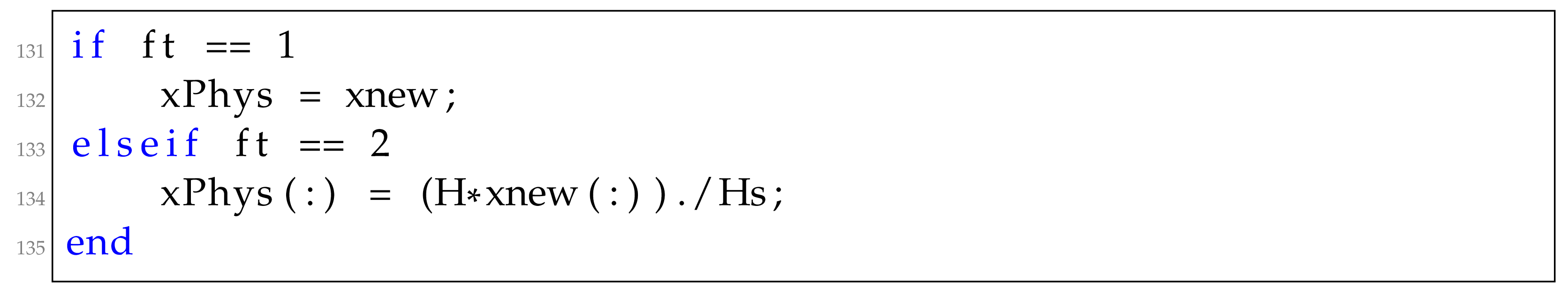
4.2. Model Order Reduction: Code Implementation

In this section, the MATLAB implementation of the three Model Order Reduction techniques are presented. A detailed description of the simple material design implementation has already been presented in previous work by the authors [17]. In this work, the three classes presented in Ref. [17] are also used; however, some new methods are added in order to enable their efficient use not only at the topology optimization formulation (macro scale) but at the homogenization one (micro scale) as well.
The features used for the implementation of the Approximate Reanalysis technique are expanded and compared to the original variant presented in Ref. [17]. Specifically, the re-initialization of the reduced basis vectors in the now updated dynamic takes into consideration the change of the value of the objective function as well as the design variables. Thus, an extra method is now used in the Approximate Reanalysis class updateBase, which is implemented as follows:
Applsci 12 10902 i028
This method performs two tasks; the first one is to check if a full dimensionality finite element analysis was performed by the solve method. If a full dimensionality one was performed, then the value of the objective function c and the design variables x are accordingly stored in the class variables c f u l l and x f u l l . In order to check if a full dimensionality analysis was performed, a class variable called s a v e is utilized, which is set to t r u e after the solution of the full dimensionality finite element analysis as follows:
Applsci 12 10902 i029
The second task of the method is activated only when a full dimensionality finite element analysis has not been performed by the solve method. In such a case, the change on the value of the objective function as well as the design variables of the current iteration are validated using two new class variables r t o l and x t o l for the objective and design variables, respectively. If either condition is validated then an indicator class variable u p d a t e is set to true. This variable is then checked inside the solve method to determine the re-initialization of the reduced basis vectors. Thus in the definition of the ar class two additional input variables are added: one for the tolerance of the change in the objective function and one for the design variables, as follows:
Applsci 12 10902 i030
In order to integrate the MOR techniques into the optimization procedure, the following changes should be applied. First, two additional input variables p 1 and p 2 are added to the UCOpt3D function, as follows:
Applsci 12 10902 i031 where p 1 defines the MOR model used in the finite element analysis on the macro scale and p 2 denotes which MOR model is used inside the homogenization method, i.e., on the micro scale. Next L i n e 87 of the UCOpt3D function is replaced with the following L i n e , applying MOR for performing the finite element analysis part:
Applsci 12 10902 i032
In addition, after the calculation of the objective function, the update of Approximate Reanalysis approach is carried out. In order to ensure that the updateBase method is accessed, an if statement is used, as follows:
Applsci 12 10902 i033
Regarding the implementation of the MOR model in the homogenization formulation, two extra methods should be added to the MOR classes. These methods are called sameSize and reinitialize. Their purpose is to reinitialize the MOR model if the active degrees of freedom of the finite element analysis in the homogenization formulation change. The change of the degrees of freedom may occur because the MOR model stays the same during the optimization procedure but the active degrees of freedom are set in each call for the homogenization method depending of the material densities values, using the following L i n e :
Applsci 12 10902 i034
The first method takes as input the size of active degrees of freedom of the finite element analysis and returns a true or false indicator by checking the size of the reduced basis vectors. The implementation is simple, as presented below:
Applsci 12 10902 i035 where s z is the number of active degrees of freedom and f i is the reduced basis matrix of the MOR model. The second method called reinitialize basically resets the MOR model without the need to recreate the model class. For the case of the Approximate Reanalysis model, this is achieved as follows:
Applsci 12 10902 i036
The re-initialization of each MOR class is different depending on each approach parameter. For the POD approach, the implementation of the reinitialize method is as follows:
Applsci 12 10902 i037 whereas for the on-the-fly approach, the implementation of the reinitialize method is as follows:
Applsci 12 10902 i038
To apply the MOR model in the homogenization method, an additional input variable p is added to the homo3DY function, as follows:
Applsci 12 10902 i039
Then, L i n e s 59 to 66 of the original homo3D are replaced with the following:
Applsci 12 10902 i040
The i f statement of the code above is utilized to check if the number of the active degrees of freedom on the current homogenization procedure is the same with the size of the reduced bases vectors of the MOR model. If the numbers does not match, a re-initialization of the MOR model is then performed using the reinitialize method. Then the MOR model is utilized to solve the finite element analysis for each of the six cases required by the homogenization function.

5. Test Examples

In this section, three test examples are presented for demonstrating the use of the proposed MATLAB code. In all test examples the three MOR models are applied and the resulting computational reduction achieved is presented. The parameters chosen for the three MOR models were chosen arbitrarily. A sensitivity analysis study performed by the authors will be presented soon [23], where the influence of the various parameters of the MOR models is examined. The three examples were chosen from the publication of the original top3D MATLAB code [3]. Although, the three examples considered to present the capabilities of the code for the material design correspond to rather simple macro domain geometries, more complex geometries for the macro domain can be dealt with as well by the code presented herein—with slight modifications. The first example refers to the classical 3D cantilever beam problem, the second example refers to the 3D wheel problem, and the third example refers to the MBB beam. The macro domains for three test examples are presented in Figure 1. For all test examples, the final form of the unit cell as well as the number of iterations required (denoted as full optimization loops in the tables) and the number of full dimensionality finite element analyses performed are provided (denoted as full optimization loops in the tables). The objective function value is presented for all three MOR approaches and without the use of any MOR model. In the second and third test examples the resulting topology of the micro scale is converted into a STL format using Ref. [24]. It is worth mentioning that in order to proceed with 3D printing of the micro structures derived through the optimization procedure and then assembling them to form the macro structure, the continuity of the unit cells when assembled to form the macro structure should be considered during the optimization phase.

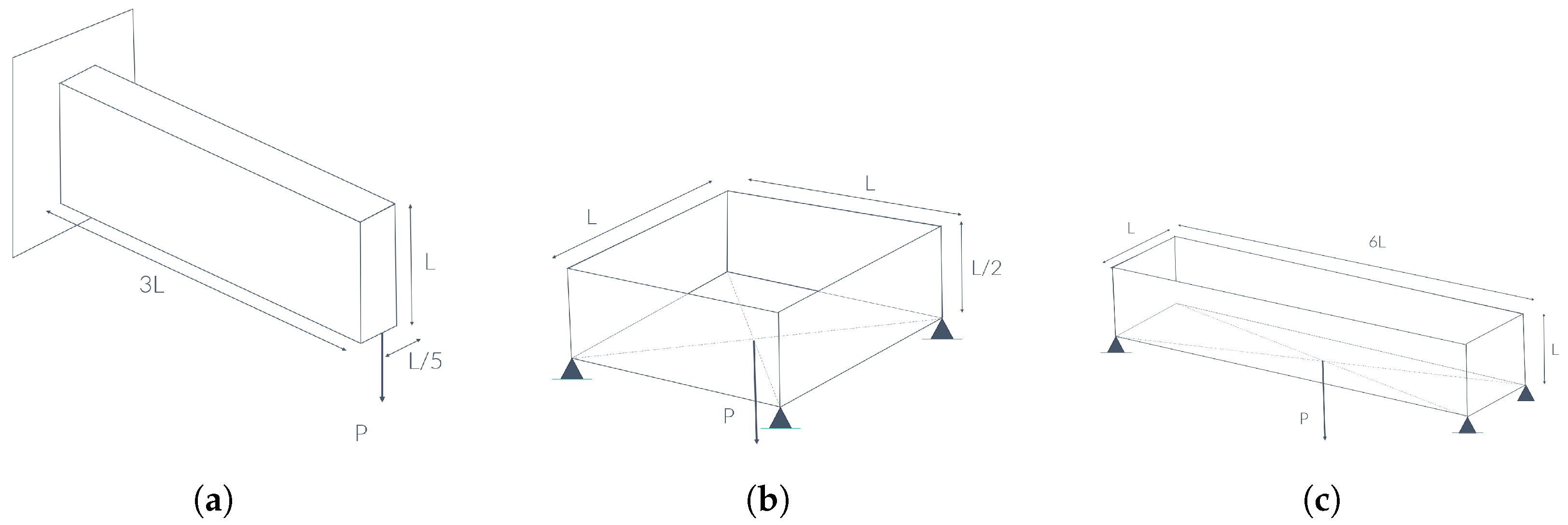
5.1. 3D Cantilever Test Example

The parameters used for the formulation of the 3D cantilever test example are as follows: a structured finite element mesh of 120 × 40 × 8 along the the abscissa, ordinate, and applicate directions was used for the discretization of the macro domain, and a 20 × 20 × 20 structured grid along the three directions for the discretization of the micro domain. In addition, the target volume was set equal to 50 % of the design domain (i.e., the micro one), the penalization factor was set equal to 3, and no filter application was set for the unit cell. Regarding the MOR models, for all three models the size of the reduced basis was set to 5 for the macro domain and to 3 for the micro domain, while the tolerance was set equal to 0.01 for both scales. For the approximate reanalysis technique, the frequency of the reduced basis update was set to 8 for the macro domain and 3 for the homogenization, and the tolerance for the compliance change and density change was set to 30 and 1.50 , respectively. The script for the implementation of the POD approach with the UCOpt3D function is presented below:
Applsci 12 10902 i041
For the implementation of the on-the-fly approach, L i n e s 1 and 2 of the above script have to be replaced, as follows:
Applsci 12 10902 i042 whereas for the implementation of the approximate reanalysis approach, L i n e s 1 and 2 of the above script have to be replaced, as follows:
Applsci 12 10902 i043
It is worth noticing that, apart from the size of the reduced basis, the remaining parameters of the MOR techniques were the same for both scales.
For the implementation of the 3D cantilever test example, the loading and boundary conditions need to be provided into the UCOpt3D function. The settings for the loading and boundary conditions are the same as those presented in Ref. [3]. Therefore, for the loading conditions, L i n e s 10 to 13 of the UCOpt3D function are set as follows:
Applsci 12 10902 i044 whereas for the boundary conditions, L i n e s 14 to 17 of the UCOpt3D function are set as follows:
Applsci 12 10902 i045
The results obtained from the three MOR techniques used for solving the topology optimization and homogenization formulations of the material design problem are presented in Table 1. The first column of Table 1 refers to the utilized MOR approach, the second column refers to the total number of optimization iterations (both full and reduced ones), the third column refers to the number of full optimization iterations, and the fourth column refers to the compliance of the resulting structure.
From the results presented in Table 1 it can be seen that the POD and on-the-fly methodologies have achieved the same values of the objective function with a small number of full dimensionality finite element analyses during the optimization procedure (i.e., macro scale) whereas the case of a typical solution of the problem with no application of any MOR technique and the use of AR for the macro scale have achieved the same objective function. The value of the objective function in the first two approaches is larger than the other two, which is due the displacement field of the objective function being approximated as well.
Regarding the MOR technique used by the homogenization function (i.e., micro scale), it was observed that, in general, out of the six finite element analyses required by every homogenization call, half of them were carried out by relying on a reduced dimensionality. The resulting topologies have small differences, and the result obtained for the POD implementation is presented in Figure 2.

5.2. 3D Wheel Test Example

Similar to the first test example, the parameters used for the formulation of the 3D wheel test example are as follows: a structured finite element mesh of 80 × 40 × 80 along the the abscissa, ordinate, and applicate directions was used for the discretization of the macro domain and a 20 × 20 × 20 structured grid along the three directions was used for the discretization of the micro domain. In addition, the target volume was set equal to 30 % of the design domain (i.e., the micro domain), the penalization factor was set equal to 3 and no filter application for the unit cell. Regarding the MOR models, for all three models the size of the reduced basis was set to 5 for the macro domain and to 3 for the micro domain, while the tolerance was set equal to 0.01 for both scales. For the approximate reanalysis technique, the frequency of the reduced basis update was set to 5 for the macro domain and 3 for the homogenization and the tolerance for the compliance change and density change was set to 30 and 1.50 , respectively. To apply the loading and boundary conditions for the 3D wheel, as described in [3], L i n e s 10 to 17 are modified, as follows:
Applsci 12 10902 i046
The results obtained from every MOR approach for the topology optimization and homogenization formulations are presented in Table 2.
Similar to the first test example from the results presented in Table 2, it can be seen that the POD and on-the-fly methodologies have achieved the same values of the objective function with a smaller number of full dimensionality finite element analyses during the optimization procedure (i.e., macro scale), whereas the case of a typical solution of the problem with no application of any MOR technique and the use of AR for the macro scale have achieved the same objective function.
Regarding the MOR technique used by the homogenization function (i.e., micro scale), it was observed that, in general, out of the six finite element analyses required by every homogenization call, half of them were carried out by relying on a reduced dimensionality. The resulting topologies have small differences. Thus, the result obtained for the on-the-fly implementation is presented in Figure 3.

5.3. MBB Beam Test Example

Similar to the first and second test example, the parameters used for the formulation of the MBB beam test example are as follows: a structured finite element mesh of 120 × 20 × 20 along the the abscissa, ordinate, and applicate directions was used for the discretization of the macro domain and a 20 × 20 × 20 structured grid along the three directions for the discretization of the micro domain. In addition, the target volume was set equal to 40 % of the design domain (i.e., the micro one), the penalization factor was set equal to 3, and no filter radius was applied. Regarding the MOR models, the parameters remained similar to the two previous test examples i.e.,the size of the reduced basis was set to 5 for the macro domain and to 3 for the micro domain, while the tolerance was set equal to 0.01 for both scales. For the approximate reanalysis technique, the frequency of the reduced basis update was set to 5 for the macro domain and 3 for the homogenization, and the tolerance for the compliance change and density change was set to 30 and 1.50 , respectively. For the application of the loading and boundary conditions, L i n e s 10 to 17 of the UCOpt3D function are modified, as follows:
Applsci 12 10902 i047
The loading and boundary conditions of these third examples are similar to the second example with the load applied at the top of the domain.
Similar to the remarks reported for the first two examples presented previously (see Table 3), the POD and on-the-fly approaches achieve the same compliance value (larger than the no MOR application) with a much smaller number of iterations. Regarding the MOR technique applied in the homogenization function from the six finite element analyses performed for each homogenization, half were computed in the reduced space. The final topologies are similar between all approaches and the topology of the POD approach is presented in Figure 4.

6. Conclusions

The scope of this work is to present a simple and easy to use implementation of the optimal design of 3D materials using the theories of topology optimization and homogenization. The presented code implementation is written suing the MATLAB code language, utilizing all its capabilities through an easy to follow implementation. To improve the computational efficiency of the optimization procedure (macro scale) and the homogenization part (micro scale), three different model order reduction (MOR) methodologies are also implemented. The integration of the MOR methodologies is general, enabling easy implementation to different applications without the need to extract them from the main script. Three different examples are presented to showcase the implementation and the efficiency of the MOR methodologies. The authors would be happy to receive suggested improvements that can be implemented in the public domain of the U C O p t 3 D codes (please address to the corresponding author by his e-mail address [email protected]).

Author Contributions

Conceptualization, G.K. and N.D.L.; methodology, G.K. and N.D.L.; software, G.K.; validation, G.K.; formal analysis, G.K.; investigation, G.K.; writing—original draft preparation, G.K. and N.D.L.; writing—review and editing, G.K. and N.D.L.; visualization, G.K.; supervision, N.D.L.; project administration, N.D.L.; funding acquisition, N.D.L. All authors have read and agreed to the published version of the manuscript.

Funding

This research was funded by funded by the European Union, NextGenerationEU, grant number OrThOP3Dics-TAEDK-06191.

Institutional Review Board Statement

Not applicable.

Informed Consent Statement

Not applicable.

Data Availability Statement

Not applicable.

Acknowledgments

This research was supported by the OrThOP3Dics project: “Topology optimization of 3D printed patient-specific spinal braces” (No: TAEDK-06191) belonging to the National Recovery and Resilience Plan, Greece 2.0 Project.

Conflicts of Interest

The authors declare no conflict of interest.

Abbreviations

The following abbreviations are used in this manuscript:
FEFinite Element
FEAFinite Element Analysis
MORModel Order Reduction
PODProper Orthogonal Decomposition
SIMPSolid Isotropic Material with Penalization
STOStructural Topology Optimization
SVDSingular Value Decomposition

References

  1. Sigmund, O. A 99 line topology optimization code written in Matlab. Struct. Multidiscip. Optim. 2001, 21, 120–127. [Google Scholar] [CrossRef]
  2. Andreassen, E.; Clausen, A.; Schevenels, M.; Lazarov, B.S.; Sigmund, O. Efficient topology optimization in MATLAB using 88 lines of code. Struct. Multidiscip. Optim. 2011, 43, 1–16. [Google Scholar] [CrossRef] [Green Version]
  3. Liu, K.; Tovar, A. An efficient 3D topology optimization code written in Matlab. Struct. Multidiscip. Optim. 2014, 50, 1175–1196. [Google Scholar] [CrossRef] [Green Version]
  4. Ferrari, F.; Sigmund, O. A new generation 99 line Matlab code for compliance topology optimization and its extension to 3D. Struct. Multidiscip. Optim. 2020, 62, 2211–2228. [Google Scholar] [CrossRef]
  5. Huang, X.; Xie, Y. A futher review of ESO type methods for topology optimization. Struct. Multidiscip. Optim. 2010, 41, 671–683. [Google Scholar] [CrossRef]
  6. Challis, V.J. A discrete level-set topology optimization code written in Matlab. Struct. Multidiscip. Optim. 2010, 41, 453–464. [Google Scholar] [CrossRef]
  7. Wang, M.; Wang, X.; Guo, D. A level set method for structural topology optimization. Comput. Methods Appl. Mech. Eng. 2003, 192, 227–246. [Google Scholar] [CrossRef]
  8. Otomori, M.; Yamada, T.; Izui, K.; Nishiwaki, S. Matlab code for a level-set based topology optimization method using a reaction diffusion equation. Struct. Multidiscip. Optim. 2014, 51, 1159–1172. [Google Scholar] [CrossRef] [Green Version]
  9. Wei, P.; Li, Z.; Li, X.; Wang, M.Y. An 88-line MATLAB code for the parameterized level set method based topology optimization using radial basis functions. Struct. Multidiscip. Optim. 2018, 58, 831–849. [Google Scholar] [CrossRef]
  10. Talischi, C.; Paulino, G.H.; Pereira, A.; Menezes, I.F.M. PolyTop: A Matlab implementation of a general topology optimization framework using unstructured polygonal finite element meshes. Struct. Multidiscip. Optim. 2012, 45, 329–357. [Google Scholar] [CrossRef]
  11. Chi, H.; Pereira, A.; Meneze, I.F.M.; Paulino, G.H. Virtual element method (VEM)-based topology optimization: An intergrated framework. Struct. Multidiscip. Optim. 2020, 62, 1089–1114. [Google Scholar] [CrossRef]
  12. Andreassen, E.; Andreasen, C.S. How to determine composite material properties using numerical homogenization. Comput. Mater. Sci. 2014, 83, 488–495. [Google Scholar] [CrossRef] [Green Version]
  13. Guoying, D.; Yunlong, T.; Yaoyao, F.Z. A 149 Line Homogenization Code for Three-Dimensional Cellular Materials Written in Matlab. J. Eng. Mater. Technol. 2018, 141, 488–495. [Google Scholar] [CrossRef]
  14. Gao, J.; Luo, Z.; Xia, L.; Gao, L. Concurrent topology optimization of multiscale composite structures in Matlab. Struct. Multidiscip. Optim. 2019, 60, 2621–2651. [Google Scholar] [CrossRef]
  15. Amir, O.; Aage, N.; Lazarov, B.S. On multigrid-CG for efficient topology optimization. Struct. Multidiscip. Optim. 2014, 419, 815–829. [Google Scholar] [CrossRef]
  16. Amir, O. Revisiting approximate reanalysis in topology optimization: On the advantages of recycled preconditioning in a minimum weight procedure. Struct. Multidiscip. Optim. 2014, 51, 41–57. [Google Scholar] [CrossRef]
  17. Kazakis, G.; Lagaros, N.D. A Simple Matlab Code for Material Design Optimization Using Reduced Order Models. Materials 2022, 15, 4972. [Google Scholar] [CrossRef]
  18. Kazakis, G.; Kanellopoulos, I.; Sotiropoulos, S.; Lagaros, N.D. Topology optimization aided structural design: Interpretation, computational aspects and 3D printing. Heliyon 2017, 3, e00431. [Google Scholar] [CrossRef]
  19. Rogkas, N.; Vakouftsis, C.; Spitas, V.; Lagaros, N.D.; Georgantzinos, S.K. Design Aspects of Additive Manufacturing at Microscale: A Review. Micromachines 2022, 13, 775. [Google Scholar] [CrossRef]
  20. Sigmund, O. Morphology-based black and white filters for topology optimization. Struct. Multidiscip. Optim. 2007, 33, 401–424. [Google Scholar] [CrossRef]
  21. Trefethen, L.N.L.N. Numerical Linear Algebra; Trefethen, L.N., Bau, D., Eds.; Society for Industrial and Applied Mathematics: Philadelphia, PA, USA, 1997. [Google Scholar]
  22. Amir, O.; Bendsøe, M.P.; Sigmund, O. Approximate reanalysis in topology optimization. Int. J. Numer. Methods Eng. 2008, 78, 1474–1491. [Google Scholar] [CrossRef]
  23. Kazakis, G.; Lagaros, N.D. Sensitivity Analysis of Model Order Reduction Parameters Applied in Topology Optimization; Technical Report; National Technical University of Athens: Athens, Greece, 2022. [Google Scholar]
  24. Tovar, A.; Liu, K. Top3dSTL. Version: 3.0. Available online: https://www.top3d.app/ (accessed on 30 August 2022).
Figure 1. The macro domains of the three considered test examples. (a) 3D Cantilever Beam test example. (b) 3D wheel test example. (c) 3D MBB beam test example.
Applsci 12 10902 g001
Figure 2. Optimized periodic unit cell for the bridge test example macro structure.
Applsci 12 10902 g002
Figure 3. Optimized periodic unit cell for the cantilever beam test example macro structure.
Applsci 12 10902 g003
Figure 4. Optimized periodic unit cell for the cantilever beam test example of the macro structure.
Applsci 12 10902 g004
Table 1. Bridge test example: Results of each MOR approach as well as the classic implementation.
ApproachTotal Optimization LoopsFull Optimization LoopsCompliance
FEA2424879.40
POD2111918.18
on-the-fly2110918.18
AR2413879.40
Table 2. 3D wheel: Results of each MOR approach as well as the classic implementation.
ApproachTotal Optimization LoopsFull Optimization LoopsCompliance
FEA3232429,740
POD2624500,120
on-the-fly2624500,120
AR3210429,740
Table 3. 3D MMB Beam: Results of each MOR approach as well as the classic implementation.
ApproachTotal Optimization LoopsFull Optimization LoopsCompliance
FEA49498762
POD26199206
on-the-fly26209206
AR50138762
Publisher’s Note: MDPI stays neutral with regard to jurisdictional claims in published maps and institutional affiliations.

