Mechanical Structure Design and Experimental Study of Gamma-ray Monitor for Small Satellite Payload

Abstract

In this paper, a novel mechanical structure for a gamma-ray monitor (GRM) is designed for a small satellite payload. Its structural stiffness, strength and dynamic response are directly related to the performance of the novel GRM, which must meet the static and dynamic characteristic requirements of the structure in a harsh vibration environment. The static and dynamic simulation of the structure are carried out by finite element method (FEM), and the mechanical structure response laws of the novel GRM are analyzed and validated by vibration tests. Through comparing the frequency response simulation results with the vibration test results, the minimum safety factor of the key components of the structure is 4.07, the fundamental frequency error is within 5.04%, the acceleration response error is within 8.5%, the root mean square of total acceleration (Grms) error is within 14.2%, and the sinusoidal characteristic sweep frequency error before and after the vibration test is within 5.0%. The results show that the payload structure has large structural stiffness, high strength and reasonable frequency response characteristics, and meets the design requirements.

1. Introduction

The GRM is a scientific instrument which can be used to detect high energy radiation phenomena in space, such as fast radio bursts, special gamma-ray bursts, magnetic star bursts, solar flares and terrestrial gamma flashes. The application of space-borne gamma-ray monitors began with the VELA satellite launched by NASA in 1963. Since then, it has gradually increased, such as the PDS detector in the BeppoSAX satellite [1], the X-ray detector (WXM) in the HETE-2 satellite [2], the gamma-ray imaging detector (GRID) in the AGILE satellite [3,4,5,6], the gamma-ray burst monitor (GBM) in the Gamma-ray Large Area Space Telescope [7], the HE detector in the Insight-HXMT satellite [8], the gamma-ray monitor (GRM) in the SVOM satellite [9], and the GRID in the CubeSats satellite [10]. These satellites are deployed in outer space and need to be loaded into the operating orbit with the launch vehicle. When designing a small satellite payload gamma-ray monitor, it is necessary to consider the impact of the harsh vibration environment of the launch vehicle. For example, Hiroyasu Tajima [11] carried out ground vibration tests of the soft gamma-ray detector on the Hitomi (ASTRO-H) satellite, and analyzed the dynamic response of its mechanical structure under conditions of vibration excitation. In the mass minimization design of the Athena WFI large-scale detector array, Jintin Frank [12] analyzed the dynamic vibration response and quasi-static acceleration load of the designed structure using the finite element method, to verify that the stress and displacement of the designed structure are within the allowable range during launch and on orbit operation. Joseph Mangan [13] performed finite element analysis for GMOD using Autodesk NASTRAN-in-cad to verify that the structure of the payload withstands the excitation during satellite launch. Liu Rui [14] conducted fundamental frequency analysis and quasi-static load analysis of eXTP satellite to verify the feasibility of the structural design. Zins [15] used MSC.NASTRAN software to analyze the structure of Hubble Space Telescope’s Wide-Field/Planetary camera (WF/PC). Jurcevich [16] performed part-level structural analysis on Soft X-ray Telescope (SXT). Yang Xue [17] estimated the mechanical performance parameters of the micro-perforated optical plate of the WXT payload on EP satellite, and carried out simulation and verification by finite element analysis. McClelland [18,19,20] performed a detailed mechanical analysis of the focusing mirror module on NASA’s International X-ray Observatory.

In order to meet the requirements of a small satellite payload mission, in this paper, a silicon photomultiplier tube (SiPM) is proposed to replace the traditional photomultiplier tube (PMT). A novel GRM mechanical structure with smaller volume and lighter weight is designed by adopting the design scheme of a central support tube structure.

2. Materials and Methods

The core of the novel GRM is a sodium iodide crystal calorimeter and SiPM. According to the requirements of the detection task, the size of the sodium iodide is Ф115 mm ×10 mm. Directly above the sodium iodide crystal is the beryllium window. The main function of the mechanical structure of the novel GRM is to maintain the external configuration of the monitor, and provide the installation space for functional modules such as calorimeter, SiPM, circuit board and independent components, as well as support and protect the internal components of the monitor.

2.1. Mechanical Structure Design of Novel GRM

The crystal support structure was designed based on the smooth shell structure of the central bearing tube, and the flange end was added outside the crystal support structure to connect with the bracket for radiant cooling plate by bolts. The design of the electronic box was based on the truss-stiffened shell structure of the central bearing cylinder, and the axial truss supporting the circuit board. A PCB board with a thickness of 2 mm was adopted, in a disc shape to facilitate the uniform layout of SiPM. Six convex ears were installed to connect with the electronic box for bolt connection. After the above fundamental design was completed, the main components were designed iteratively and corresponding models were corrected in real-time to obtain the preliminary design. A rabbet was designed at the junction of the crystal support structure and the electronic box to ensure the electromagnetic shielding of the structure. The photoconductive glass was bonded to the sodium iodide crystal and crystal support structure through GN522 adhesive. In addition to the electronic box using aluminum alloy 2A12-H112, the other mechanical structure of the novel GRM adopted magnesium alloy ZK61M. The weight of the novel GRM is about 750 g, and the external size is Ф146.6 mm × 32.8 mm, as shown in Figure 1a.

2.2. Comparison of Traditional and Novel GRM

The traditional gamma-ray detector with PMT is shown in Figure 1b. Its size and weight are about Ф190 mm × 300 mm and more than 4 kg, respectively. Comparing with the traditional gamma-ray detector, the novel GRM has the advantages of: compact structure, vibration resistance, small size, light weight and no need for high pressure, thus the cost of manufacturing and loading orbit can be reduced.

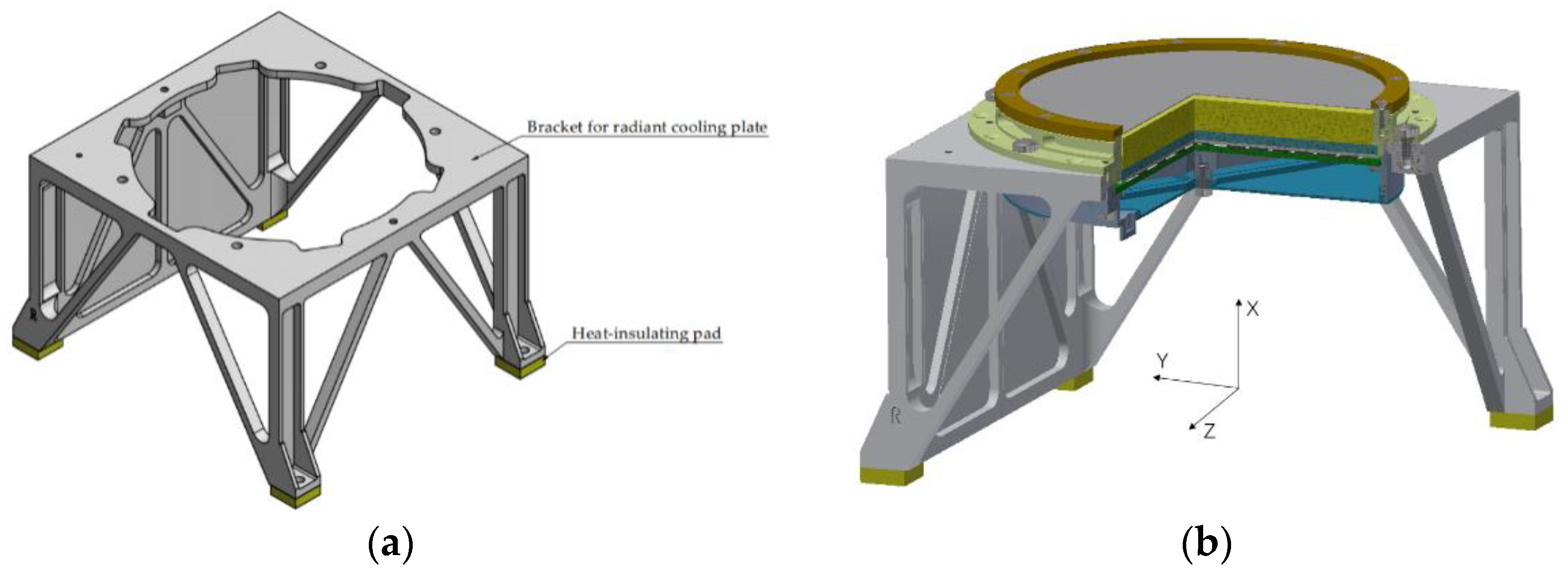
2.3. Mechanical Structure Design of the Bracket for the Radiant Cooling Plate

The main function of the bracket for the radiant cooling plate is to support the novel GRM and heat transfer, which requires sufficient strength and stiffness. Therefore, a frame structure was adopted to ensure its mechanical and thermal performance requirements. The novel GRM was installed with a satellite insulation layer made of FR4, and the thermal insulation pad was added at the four corners of the bracket. In order to better transfer thermal energy, the bracket is closed at the +Y side of the star. The flatness of the closed surface is 0.1 mm/100 mm × 100 mm, and the roughness is 3.2 µm to ensure thermal conductivity. The bracket for the radiant cooling plate was made using magnesium alloy ZK61M and its mass is about 250 g. The structure is shown in Figure 2a, and the whole assembly of the novel GRM is shown in Figure 2b.

Jimenez-Martinez, Moises [21] used feedforward ANN and synthetic data to predict the strength of the structure. In order to ensure that the mechanical structure of the novel GRM meets the requirements of the space-borne environment during the process of ground transportation to launch flight, the overload analysis, modal analysis sinusoidal vibration analysis, random vibration analysis and related experimental research were carried out. By combining the data of the sinusoidal characteristic sweep frequency test with the parameter method, the correction of the damping coefficient in the finite element model was modified to reduce the calculation error of the FEM and obtain reliable dynamic response prediction results [22,23].

3. Modeling

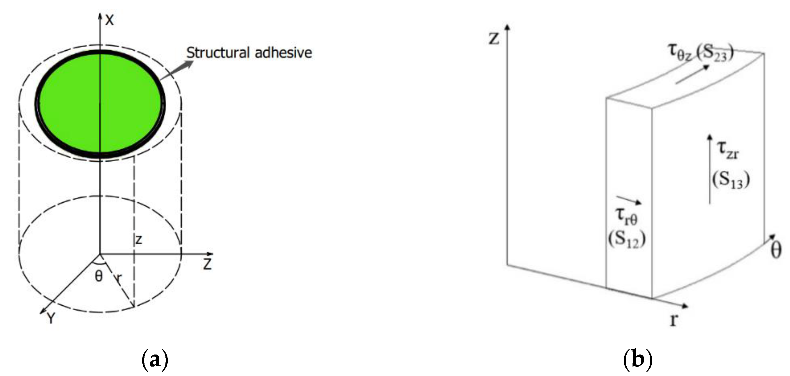
3.1. Structural Finite Element Static Analysis Equations

Structural static analysis mainly studies the mechanical behavior of satellite structures under static or quasi-static load conditions to solve the static strength, stiffness, and stability problems of the structure. Based on the assumption of small deformation, the fundamental equations of the finite element displacement method for static analysis are established [24].

$$\left[K\right]\left\{u\right\}=\left\{F\right\}$$

(1)

where $\left[K\right]$ is the stiffness matrix.

By solving the above equations, the displacement vector $\left\{u\right\}$ is obtained at each point. According to the displacement interpolation function, the relationship between strain and displacement and the relationship between strain and stress are given in elastic mechanics. The strain and stress of the unit nodes are expressed as:

$$\left\{{\epsilon }^d\right\}=\left[B\right]\left\{u\right\}-\left\{{\epsilon }^{th}\right\}$$

(2)

$$\left\{\sigma \right\}=\left[D\right]\left\{{\epsilon }^d\right\}$$

(3)

where $\left\{{\epsilon }^d\right\}$ is the structural strain vector, $\left\{{\epsilon }^{th}\right\}$ is the thermal strain vector, $\left[B\right]$ is the strain-displacement conversion matrix of the nodes, and $\left[D\right]$ is the elasticity coefficient matrix.

3.2. Structural Finite Element Dynamic Analysis Equations

3.2.1. Modal Analysis Equations

The mathematical basis of modal analysis is the eigenvalue problem of dynamic motion equations. The system is regarded as a linear element, and assuming that its structure is not affected by load and stability, that is, the stiffness and mass are constant, the dynamic equations of undamped free vibration are as follows [25]:

$$\mathrm{M}\ddot{x}\left(t\right)+Kx\left(t\right)=0$$

(4)

$$K-{\omega }^{2}M\mathsf{Ф}=0$$

(5)

where $M$ is the mass matrix, $x\left(t\right)$ is the system displacement vector as a function of time, $\ddot{x}\left(t\right)$ is the acceleration vector function, $\omega$ is the intrinsic frequency, and $\mathsf{Ф}$ is the modal vibration pattern.

The natural frequency 𝜔_𝑖 (𝑖 = 1, 2, …, 𝑛) of the system can be obtained by solving the above equation and the corresponding modal vibration pattern ${\mathsf{Ф}}_i\left(i=1,2,\dots ,n\right)$.

3.2.2. Sinusoidal Vibration Analysis Equations

Sinusoidal vibration analysis is for the purposes of studying the dynamic response of a structure under a series of periodic loads in the form of sine or cosine, and is mainly used to characterize the amplification effect of the structure on the external loads at different frequencies. For the dynamic response characteristics of the system, the modal superposition method is usually used to solve the external excitation. The solution formula is given by [26]:

$$y\left(t\right)=\mathsf{Ф}q\left(t\right)={{\displaystyle \sum }}_{j=1}^n{q}_j{\mathsf{Ф}}_{\mathrm{j}}$$

(6)

where $y\left(t\right)$ is the system displacement as a function of time, ${\mathsf{Ф}}_j$ is the first order damped self-oscillation, and $q_j$ is the oscillation coordinate, representing the weighting factor of the oscillation. The generalized motion equation is obtained by multiplying the above equation with ${\mathsf{Ф}}^T$:

$$M^{*}\ddot{q}\left(t\right)+C^{*}\dot{q}\left(t\right)+K^{*}q\left(t\right)=F^{*}$$

(7)

where $q\left(t\right)$ is the nodal displacement as a function of time, $M^{*}$ is the mass matrix, $C^{*}$ is the damping matrix, $K^{*}$ is the stiffness matrix, and $F^{*}$ is the external load.

Equation (7) is decomposed into n independent single degree of freedom equations of motion:

$${\ddot{q}}_j+2{\zeta }_j{\omega }_j{\dot{q}}_j+{\omega }_j^2{q}_j=\frac{F_j^{*}}{m_j^{*}}$$

(8)

The solution of the above equation represents the displacement, velocity and acceleration, so as to measure the dynamic response of the system. For simple harmonic vibration, the dynamic equation of the system is:

$$M\ddot{y}\left(t\right)+C\dot{y}\left(t\right)+Ky\left(t\right)=-ME{x}_0$$

(9)

where $E$ is the elasticity modulus of the material, and $x_0$ is the excitation displacement vector. The generalized equation can be obtained as:

$$M^{*}\ddot{q}\left(t\right)+C^{*}\dot{q}\left(t\right)+K^{*}q\left(t\right)=-\gamma x_0{e}^{j\omega t}$$

(10)

where $\gamma$ represents the equation feature vector.

At this time, the frequency response matrix of the system is:

$$H\left(\omega \right)={\left(K-{\omega }^{2}M+i\omega C\right)}^{-1}$$

(11)

thus, the steady-state solutions of the equation are obtained as:

$$y\left(t\right)={{\displaystyle \sum }}_{j=1}^n{q}_j{\mathsf{Ф}}_j={{\displaystyle \sum }}_{j=1}^n-{\gamma }_j{H}_j{\mathsf{Ф}}_j{x}_j{e}^{j\omega t}$$

(12)

$$\ddot{y}\left(t\right)=-{\omega }^2{{\displaystyle \sum }}_{j=1}^n-{\gamma }_j{H}_j{\mathsf{Ф}}_j{x}_j{e}^{j\omega t}$$

(13)

In Equation (13), $\ddot{y}\left(t\right)$ is the response acceleration of some point to external excitation.

3.2.3. Random Vibration Analysis Equations

Random vibration analysis uses statistical methods to study the excitation or response of a random vibration system, and to calculate the displacement, stress, strain and reaction of the model based on power spectral density (PSD). PSD describes the variance of excitation or response varying with frequency.

Random vibration is uncertain, and the dynamic equation is solved by approximately converting the random excitation into the simple harmonic excitation:

$$M\ddot{y}\left(t\right)+C\dot{y}\left(t\right)+Ky\left(t\right)=-ME\ddot{x}\left(t\right)$$

(14)

where $\ddot{x}\left(t\right)$ is the second derivative of the displacement vector.

The steady-state solution of the above equation is:

$$\widehat{y}\left(t\right)={{\displaystyle \sum }}_{j=1}^n{q}_j{\mathsf{Ф}}_j=-{\gamma }_j{H}_j{\mathsf{Ф}}_j\sqrt{k_{xx\left(\omega \right)}}{e}^{j\omega t}$$

(15)

and the power spectral density is obtained by solving the following equation:

$$K\left(\omega \right)=\widehat{y}\left(t\right)\widehat{y}{\left(t\right)}^T\approx {{\displaystyle \sum }}_{j=1}^n{\gamma }_j^2{\mathsf{Ф}}_j{\mathsf{Ф}}_j^T{\left|H_j\left(\omega \right)\right|}^2{K}_{xx}\left(\omega \right)d\omega$$

(16)

thus, the Grms response can be obtained as:

$$A={\left[{{\displaystyle \int }}_{-\infty }^{+\infty }K\left(\omega \right)d\omega \right]}^{\frac{1}{2}}={\left[{{\displaystyle \sum }}_{j=1}^n{\gamma }_j^2{\mathsf{Ф}}_j{\mathsf{Ф}}_j^T{\left|H_j\left(\omega \right)\right|}^2{K}_{xx}\left(\omega \right)d\omega \right]}^{\frac{1}{2}}$$

(17)

The PSD of the structure in the prescribed frequency domain is calculated by random vibration analysis to measure the response.

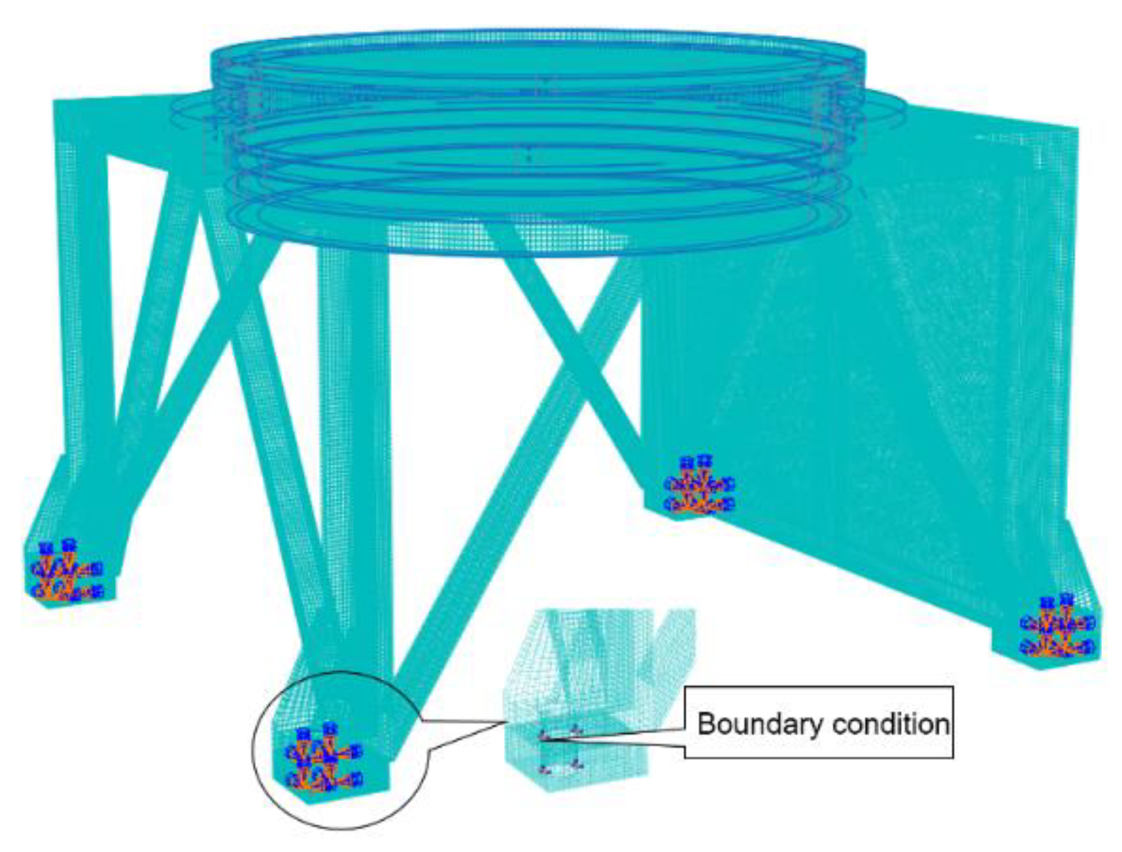
3.3. Establishment of Finite Element Model to the System

The finite element model is established using the module modeling strategy. According to the structure composition, the novel GRM mechanical system was divided into three modules: crystal assembly, electronic box assembly and bracket assembly. Each module is decomposed and modeled again according to its own auxiliary equipment. After the modular modeling was completed, the bonding and bolt connection were simulated using the connection constraint or multi-point constraints (MPC) algorithm, and then each module was assembled into a finite element model of the overall structure, as shown in Figure 3. It is necessary to simplify the actual structure, in order to make element calculations feasible in the process of establishing the model [27,28,29], such as the simplification of the SiPM components and the cover of the electronic box, the weight being applied to the electronic box. The complexity of the overall structure when meshing was also considered, in order to use more accurate hexahedral cells for finite element calculations. For parts that could not be meshed directly using the “Structured” mesh in ABAQUS, “Sweep” was used for meshing, but this resulted in malformed cells in transition zones or in narrow edges. FEM with deformed meshes were used to balance the following three factors: (1) They allow more detailed geometric features of the representation model. (2) The mesh size of FEM affects CPU computing time [30]. (3) When the contact area mesh is refined, the coarse mesh can better transition to the fine mesh. In order to avoid the distortion of the calculation results caused by the abnormal cells appearing in the key area, during the finite element calculation, the abnormal cells appear in the non-key area by adjusting the mesh density of the whole model and refining the mesh of the contact area. Through the above adjustment, it was found that the FEM used in this paper reached the convergence of the calculation results, and the FEM was effective. The FEM was also proved to be effective by comparing with the experiment in Section 4.2.1. Thus, in this case, although the model had deformed units, the accuracy of the results met the calculation requirements. The number of elements and deformation rate are shown in

Table 1. Model element information.

Structure	Number of Elements	Number of Deformed Elements	Deformed Ratio (%)
Bracket for radiant cooling plate	333,632	12,486	3.7
Crystal box	37,095	1734	4.67
Sodium iodide crystal	15,930	0	0
Quartz	6844	0	0
Be sheet	25,464	0	0
Be sheet gland	4943	0	0
Structural adhesive 1	12,574	174	1.384
Structural adhesive 2	1128	0	0
Electronic box	93,619	1592	1.7
Heat-insulating pads	8620	0	0
Total	539,849	15,968	2.96

.

3.4. Material Parameters

The material [31,32] selection in the novel GRM is shown in

Table 2. Material parameters of each component for the novel GRM assembly.

Component	Materials	Density (g/cm3)	Elastic Modulus (E/MPa)	Poisson’s Ratio	Tensile Strength (MPa)
Bracket for radiant cooling plate	ZK61M	1.8	43,000	0.34	280
Electronic box	2A12-H112	2.8	68,000	0.33	390
Sodium iodide crystal	NaI	3.671	20,000	0.314	/
Be sheet	Be	1.85	290,000	0.08	180
Be sheet gland	ZK61M	1.8	43,000	0.34	280
Crystal box	ZK61M	1.8	43,000	0.34	280
Quartz	K9	2.51	82,000	0.206	1050
Structural adhesive	GN522	1.03	1.2	0.48	2 (Shear stress)
Heat-insulating pad	FR4	1.8	25,000	0.2	300

, where the non-metallic material parameters were provided by the Laboratory of the Institute of High Energy Physics, Chinese Academy of Sciences.

3.5. Load and Boundary Conditions

According to the DRO satellite system on-board product test conditions document, KSW-DRO-E03-2021, the product is required to withstand sinusoidal vibration, random vibration and other mechanical environments without failure or damage. The mechanical test conditions corresponding to the identification level are shown in

Table 3. Sinusoidal vibration test conditions.

	Frequency Range (Hz)	Vibration Magnitude (o-p) g	Sweep Frequency Direction	Loading Rate
Quasi-accreditation level	5–15	13.8 mm	X, Y, Z	2 oct/min
	15–100	12.5 g

and

Table 4. Random vibration test conditions.

	Frequency Range (Hz)	Acceleration Power Spectral Density	Grms (g2/Hz)	Direction	Vibration Time
Quasi-accreditation level	10–150	+6 dB/oct.	10.575	X, Y, Z	180 s/direction
	150–800	0.0782 g2/Hz
	800–2000	−3 dB/oct.

.

In the ground vibration experiment at the scheme design stage, the fixed mode of the novel GRM is shown in Figure 4. According to the position of the screw hole constrained by the model in the vibration test, the six degrees of freedom of the inner surface of the four mounting holes at the bottom of the convex ear are simplified by the constraint in theoretical analysis, as shown in Figure 5.

According to the prediction of dangerous parts and concerned areas, considering the structural characteristics, the acceleration sensors are arranged at the flange end of the crystal shell in the vibration test, as shown in Figure 6. The corresponding positions of the sensors are arranged in the vibration test, and are selected as the sampling points in the theoretical analysis.

4. Simulation and Experimental Results

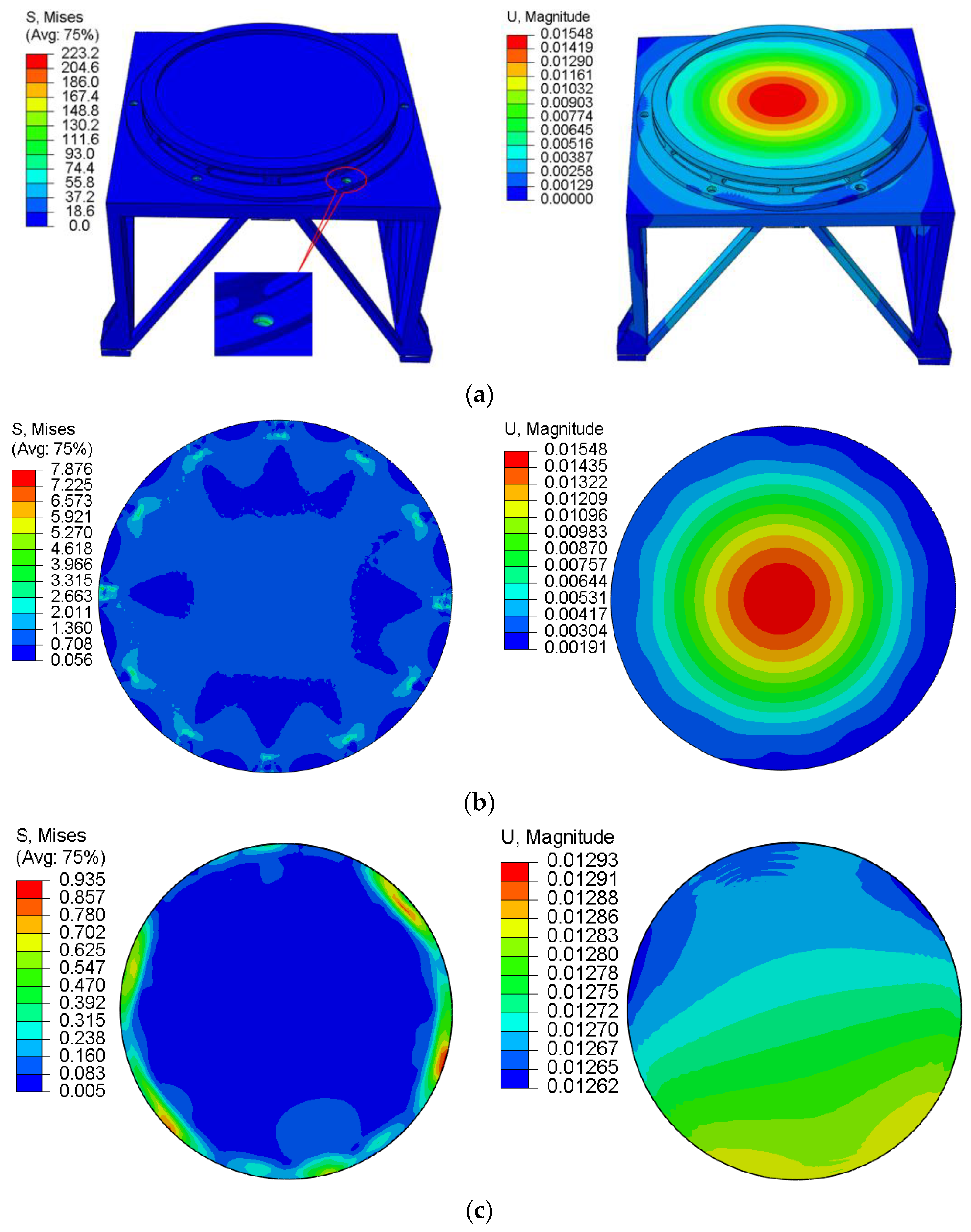
4.1. Static Analysis

In order to verify the static characteristics of the product under overload conditions, its strength is evaluated on the basis of transportation conditions of the identification level: (1) maximum axial (X-direction) overload of the satellite: 12 g; and (2) maximum lateral (Z-direction and Y-direction) overload of the satellite: 9 g.

According to the detailed design requirements of the satellite payload system, the safety factor corresponding to the yield strength of the structure is 1.5. Since it is difficult to predict the overload conditions in all directions during transportation, under the combined action of the above maximum overload conditions, the overload environment estimated by the model is more serious than the actual situation, and the calculation results are relatively safe. In this overload analysis, the stress and displacement results of the structural adhesive, photoconductive glass and beryllium sheet are focused on, as shown in Figure 7.

In order to obtain the shear stress of the structural adhesive conveniently, a mathematical model was established according to its distribution and shape characteristics, as shown in Figure 8. The r-axis and z-axis respectively correspond to the Y-axis and X-axis of the original coordinate system, and the positive direction of the $\theta$-axis is determined according to the right-handed rule. The shear stress ${\mathsf{\tau }}_{r\theta },{\tau }_{\theta z}$ and ${\tau }_{rz}$ of the structural adhesive correspond to S₁₂, S₂₃ and S₁₃ in the ABAQUS coordinate system, respectively. The maximum von Mises stress and safety margin of key parts are shown in

Table 5. Overload analysis results.

Name	Materials	Maximum Stress (MPa)	Safety Margin (MS)
Structural adhesive	GN522	0.263	4.07
Photoconductive glass	K9	0.94	>10
Beryllium sheet	Be	7.88	>10

.

The calculated minimum safety margin of the structural adhesive is 4.07, which is greater than the minimum bearing strength requirement of non-metallic materials of 0.25. The distance between the beryllium sheet and the sodium iodide crystal is 1.3 mm, and the maximum displacement of the beryllium sheet is 15.48 µm, which will not interfere with the sodium iodide crystal. Therefore, the structural strength and stiffness meet the design requirements under overload conditions.

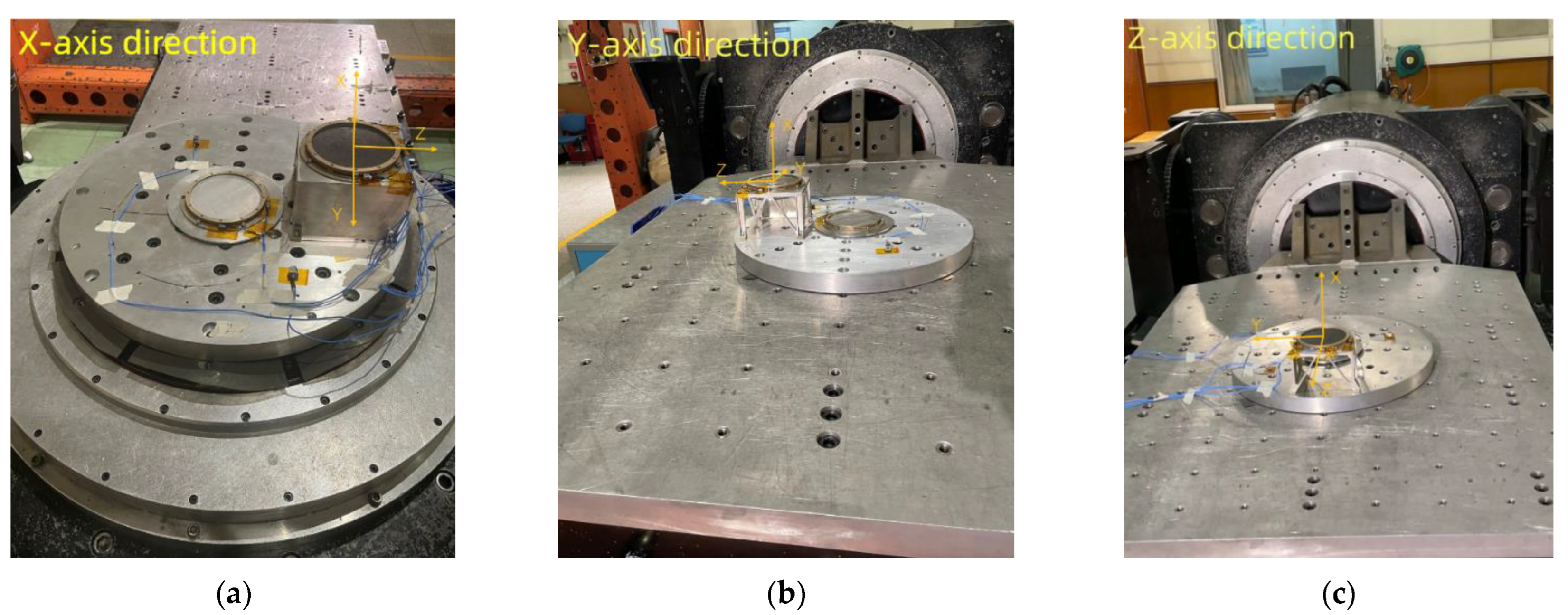
4.2. Dynamical Analysis

4.2.1. Modal Analysis

The first step in performing a dynamic analysis is determining the structure’s natural frequencies and mode shapes, taking zero damping into account. The results of this analysis define the structure’s dynamic behavior and can be used to predict how the structure will respond to dynamic loads [33]. Before the vibration test, the fundamental frequency of the structure was obtained through a 0.5 g sinusoidal characteristic sweep frequency test within the frequency range of 10–2000 Hz. The first four order natural frequencies and vibration modes of the novel GRM are shown in Figure 9. The sinusoidal sweep frequency test curves in X, Y and Z directions before the vibration test of each measuring point are shown in Section 4.2.2. The first order main frequencies in X, Y and Z directions obtained by the simulation analysis and test results are shown in

Table 6. Modal data.

Direction	Modal Analysis (Hz)	Modal Test (Hz)	Relative Error
X	732.34	771.19	5.04%
Y	420.25	436.25	3.67%
Z	615.66	586.07	−4.80%

.

The first order main vibration mode frequency of modal analysis is 420.25 Hz, which is greater than the 100 Hz specified by the spacecraft [34], indicating that the stiffness of the main structure of the designed model meets the design requirements. From the test sinusoidal characteristic sweep frequency curve in Figure 10, it can be seen that the first order frequency of the novel GRM is 771.19 Hz in X direction, 436.25 Hz in Y direction, and 586.07 Hz in Z direction. Combined with the above modal analysis results, the relative errors are obtained, as shown in Table 6. As can also be seen from Table 6, the results of the three directions obtained by the modal analysis and the test results are all within the allowable error range of 10% in the engineering analysis, indicating that the established finite element model is effective and has a sufficient safety margin.

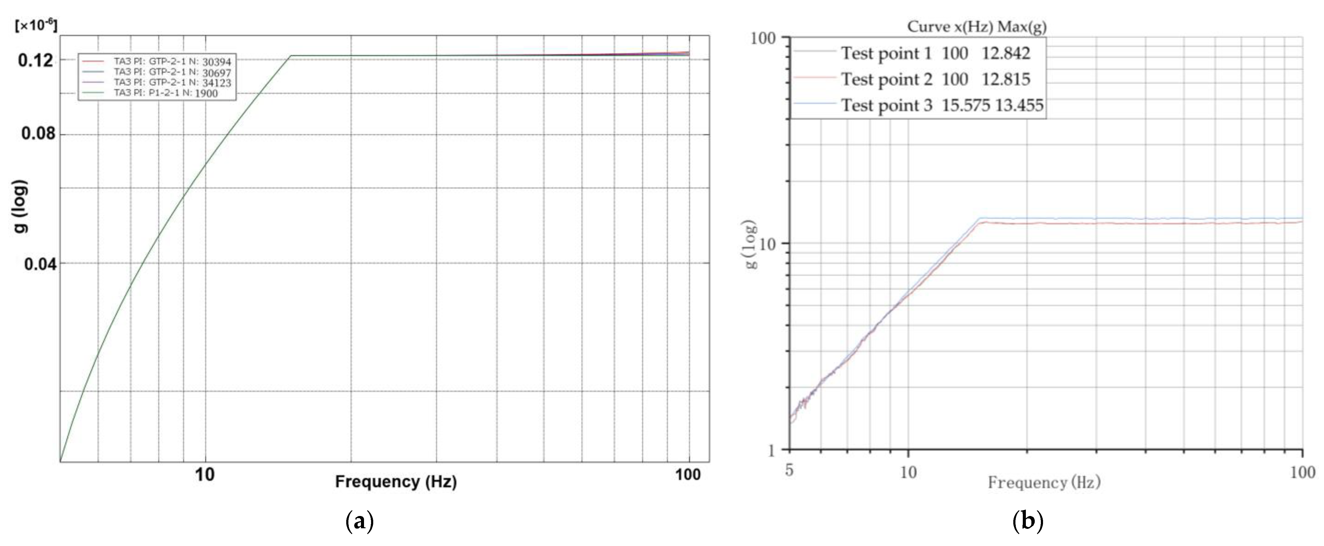
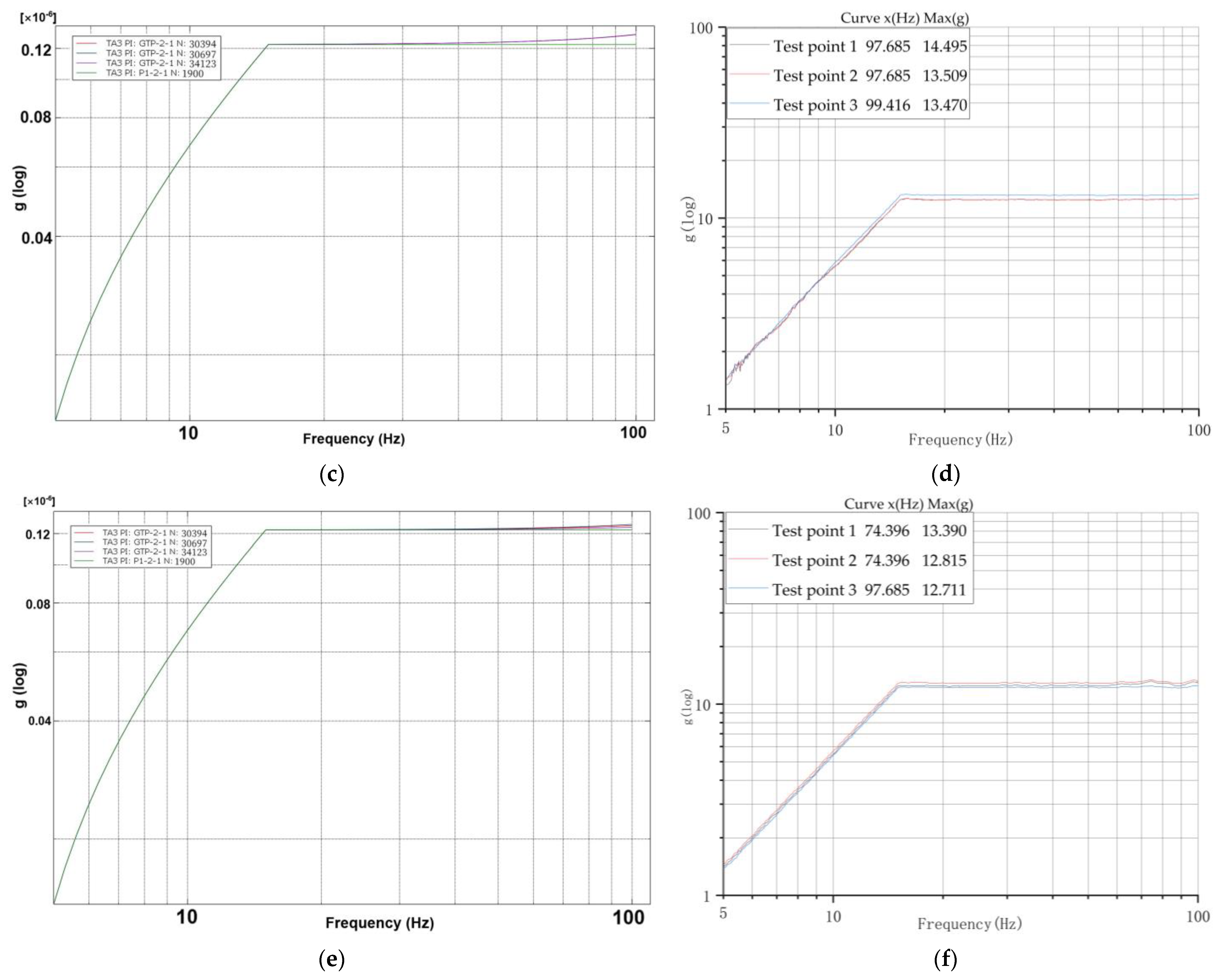
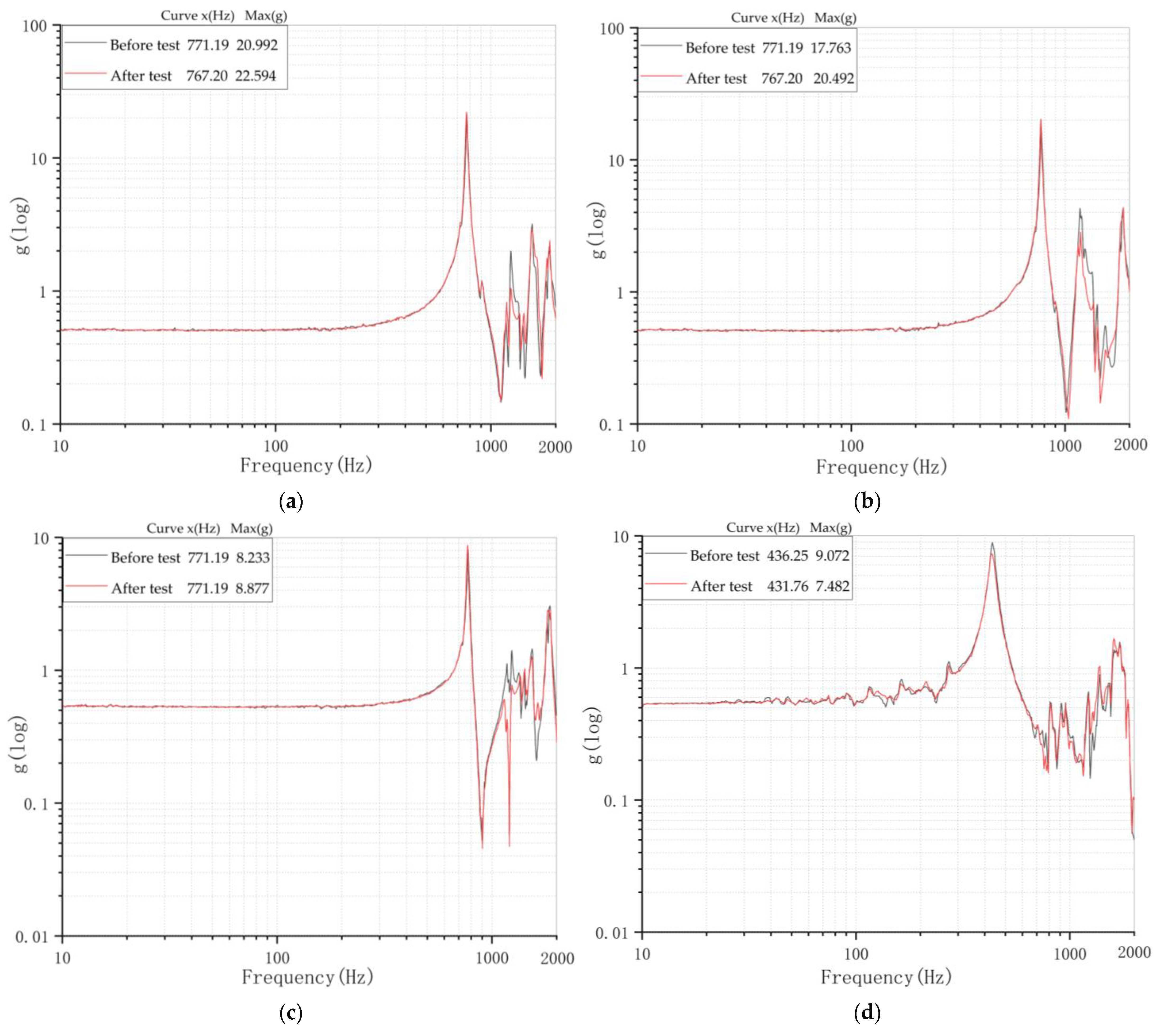
4.2.2. Sinusoidal Vibration Analysis

The sinusoidal vibration analysis model is consistent with the model of modal analysis. The damping ratio of the product structure is taken as the empirical value of 0.03, and the test conditions listed in Table 3 are used as the load input. The excitation frequency of the satellite engine is generally less than 100 Hz. In order to understand the dynamic performance of the model under this excitation, sinusoidal vibration analysis is carried out. The acceleration response curves obtained by FEM and test are shown in Figure 11.

From comparison of the finite element analysis and experimental data, the relative error of the acceleration amplification factor Q is shown in

Table 7. Comparison of theoretical analysis and experimental test acceleration response data.

Measurement Points	Categories	X-Direction		Y-Direction		Z-Direction
		g	Magnification	g	Magnification	g	Magnification
1	Analysis	12.67	1.01	13.27	1.06	12.91	1.03
	Test	12.84	1.03	14.5	1.16	13.39	1.07
	Error	1.3%		8.5%		3.6%
2	Analysis	12.75	1.02	13.25	1.06	12.82	1.03
	Test	12.82	1.03	13.51	1.08	12.82	1.03
	Error	0.5%		1.9%		0%
3	Analysis	12.59	1.01	13.27	1.06	12.69	1.015
	Test	13.46	1.08	13.47	1.077	12.71	1.02
	Error	6.5%		1.5%		0.1%

. Combining with Table 7 and Figure 11, it can be found that the amplification factors in X, Y and Z directions of the test are consistent with the trends of the finite element analysis results. The overall excitation curve of the test is consistent with the FEM curve, there is no obvious peak, and the amplification factor of the acceleration response is also within the reasonable range of engineering requirements.

After the identification level sinusoidal vibration test, the novel GRM must be subjected to the 0.5 g sinusoidal characteristic sweep frequency test. By comparing sweep frequency results before and after the sinusoidal vibration test, it is verified whether the structure is damaged under the excitation of sinusoidal vibration conditions. The results are shown in Figure 10.

From the sinusoidal characteristic sweep frequency of each measuring point in X, Y and Z directions in Figure 10, it can be seen that the sweep frequency curves of each measuring point before and after the sinusoidal vibration test are consistent. Before and after the identification level sinusoidal vibration experiment, the frequency of the first order main frequency in X and Y directions does not change, and the drift value of the first order main frequency in Z direction is less than 5.0%. Under sinusoidal excitation, the structure can be kept intact, indicating that the strength of the structure design meets the requirements under low frequency.

4.2.3. Random Vibration Analysis

On the basis of modal analysis, the damping ratio was taken as 0.03, and the test conditions listed in Table 4 were used as load input to calculate the response of the product under random excitation in X, Y and Z directions. In the random vibration test, the excitations of each frequency component acts simultaneously on the satellite structure at any time, so it is impossible to predict its instantaneous vibration variation law. Generally, statistics such as root mean square, cumulative root mean square and PSD curve are used to study the random vibration of the satellite structure [35]. The acceleration power spectral density curves of FEM and experiment are shown in Figure 12.

The acceleration PSD curve of measuring points 1–3 is shown in Figure 12. The first peak in X direction is 755 Hz and 732 Hz in test and finite element analysis, respectively; the first peak in Y direction is 425 Hz and 420 Hz in test and finite element analysis, respectively; the first peak in Z direction is 547 Hz and 615 Hz in test and finite element analysis respectively; and the fundamental frequency error of each measuring point direction meets the engineering requirements. The peak and valley number of PSD in 200–1000 Hz is basically consistent with the experimental curve. There is an obvious difference between the theoretical curve and the experimental curve of PSD in the high frequency band of 1000–2000 Hz, and the reasons for the deviation are analyzed as follows:

(1)

The deviation of finite element modeling. In order to simplify the finite element calculation, the tie constraint and MPC algorithm are used to simulate the screw connection, so that the stiffness of the connection area is deviated from the actual stiffness. This is also the reason for the deviation between the natural frequencies obtained by the analysis of the test in each stage.

(2)

Uncertainty of modal damping selection. In the process of finite element simulation and calculation, the damping value was adopted the empirical value of 0.03, which deviates from the actual damping value of the model.

(3)

Test error. In the test stage, there is a coupling effect in the transmission process of random excitation applied by the vibration platform. There are deviations between the idealized treatment of factors (such as inter-part friction and inter-part clearance) and the random vibration test.

(4)

High frequency characteristics are more sensitive to structural details, and the finite element mesh needs to be gradually encrypted with the increase in frequency band width, but the calculation scale will expand rapidly, so the high frequency numerical results have large errors [36].

In the finite element analysis of this paper, according to experience, the initial value of damping is taken as 0.03, and there is a large error between the total root mean square of the acceleration analysis results and the experimental results, as shown in

Table 8. PSD response before model correction.

Measurement Points	Categories	X-Direction		Y-Direction		Z-Direction
		Grms (g2/Hz)	Magnification	Grms (g2/Hz)	Magnification	Grms (g2/Hz)	Magnification
1	Analysis	37.50	3.55	29.07	2.75	32.66	3.09
	Test	56.16	5.31	29.31	2.77	54.29	5.13
	Error	−33%		−0.8%		−39.8%
2	Analysis	27.90	2.64	29.81	2.82	46.98	4.44
	Test	57.04	5.39	25.81	2.44	47.31	4.47
	Error	−51%		15%		−0.7%
3	Analysis	15.85	1.50	29.80	2.82	23.95	2.26
	Test	25.32	2.39	33.16	3.14	29.69	2.81
	Error	−37%		−10%		−19%

. Therefore, the parameter method is adopted for the finite element model correction. According to the sweep frequency test results of sinusoidal characteristic in Figure 10 and the half-power bandwidth method [37], the damping value in X direction is 0.013, while the values are 0.029 in Y direction and 0.02 in Z direction, respectively. The damping value obtained by the 0.5 g sweep frequency is used as the input parameter of structural damping, and the random vibration analysis is carried out after the finite element model is modified. The corrected values are compared with the experimental values, as shown in

Table 9. PSD response after model correction.

Measurement Points	Categories	X-Direction		Y-Direction		Z-Direction
		Grms (g2/H)	Magnification	Grms (g2/Hz)	Magnification	Grms (g2/Hz)	Magnification
1	Analysis	50.35	4.76	30.16	2.85	57.90	5.48
	Test	56.16	5.31	29.31	2.77	54.29	5.13
	Error	−10.4%		2.9%		6.6%
2	Analysis	57.67	5.45	29.4	2.78	42.90	4.06
	Test	57.04	5.39	25.81	2.44	47.31	4.47
	Error	1.1%		13.9%		−9.3%
3	Analysis	28.93	2.74	30.10	2.85	29.81	2.82
	Test	25.32	2.39	33.16	3.14	29.69	2.81
	Error	14.2%		−9.2%		0.4%

. It can be seen from Table 9 that the overall errors between the model correction results and the experimental results are reduced, which indicates the effectiveness of the finite element model correction and provides guidance for the subsequent optimization design.

After the identification level random vibration test, a 0.5 g sinusoidal characteristic sweep frequency test was conducted to verify the integrity of the structure. The results are shown in Figure 13.

From the sinusoidal characteristic sweep frequency curves before and after the random vibration test of measuring points in X, Y and Z directions in Figure 13, it can be concluded that the sweep frequency curves of each measuring point before and after the random vibration test coincide well. The frequency drift of the first order dominant frequency is less than 1.0% before and after the random vibration experiment at the X identification level, while the same drift in Y direction is less than 2.0% and the drift in Z direction is less than 5.0%. The structure is therefore safe and meets the requirements under random excitation.

5. Discussion

According to the dynamic simulation and experimental results, it can be concluded that the response of sinusoidal vibration is much smaller than that of random vibration. The reason is that the basic frequency of the structure calculated in Section 4.2.1 is 420.25 Hz, and the excitation condition of sinusoidal vibration is 5–100 Hz, which will not cause obvious resonance response. From this perspective, it seems that the sinusoidal vibration test is unnecessary. In fact, sinusoidal vibration test can be equivalent to a quasi-static inertial force process, simulating low frequency transient events.Sinusoidal vibration is the actual working state of satellite from ignition to orbit loading, especially in the atmosphere. The structure must undergo the test of this working condition, otherwise it is impossible to predict whether the structure or internal components will be damaged in this process.

Because the integrity of sodium iodide crystal and structural adhesive in the novel GRM cannot be judged intuitively in the process of finite element analysis and mechanical vibration test. Therefore, before the mechanical test, the photomultiplier tube (PMT) is used to test the performance of the crystal package, as shown in Figure 14a. The energy spectrum before the test is shown in Figure 14b. Through the analysis of the data in the energy spectrum diagram, it is found that the half-peak width size meets the requirements of the DRO satellite file KSW-DRO-Q09-2021, indicating that the sodium iodide crystal has a good energy resolution for gamma rays. Then it is considered that there are no cracks or defects in the bonding site at this time. After the mechanical vibration test, PMT was used again to test the performance of the crystal package. The energy spectrum after the test is shown in Figure 14b. Comparing the mechanical test before and after the vibration of the crystal packaging performance test found that the two full-energy peaks almost coincide, obtained before and after the mechanical vibration test structural adhesive and sodium iodide crystal does not exist cracks or defects.

6. Conclusions

The mechanical design of small satellite GRM payload is completed, comparing with the traditional gamma-ray detector, the novel GRM has the advantages of compact structure, vibration resistance, small size, light weight and no need for high pressure. The finite element model was established by using ABAQUS, and the overload analysis, modal analysis, sinusoidal vibration and random vibration response analysis were completed, and the relevant ground vibration tests were carried out. The conclusions are as follows:

(1)

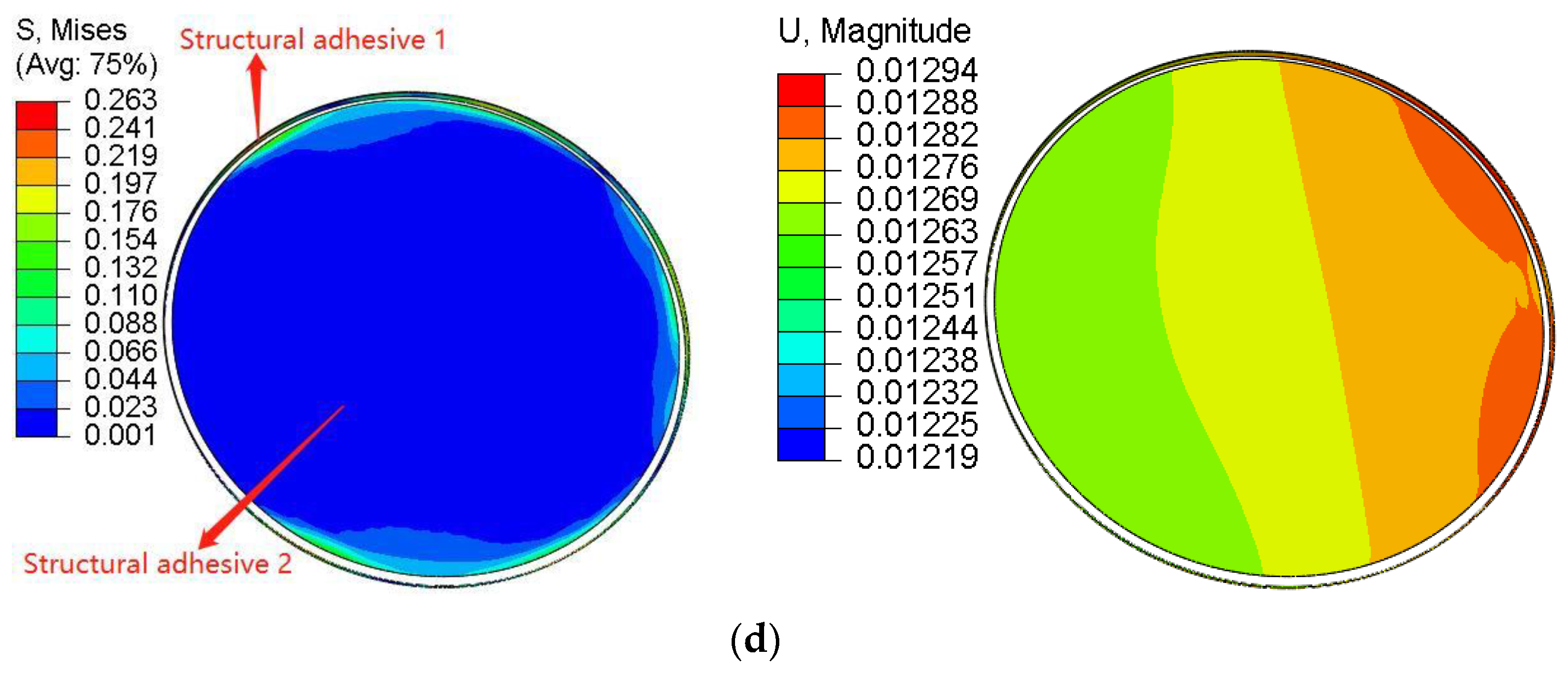
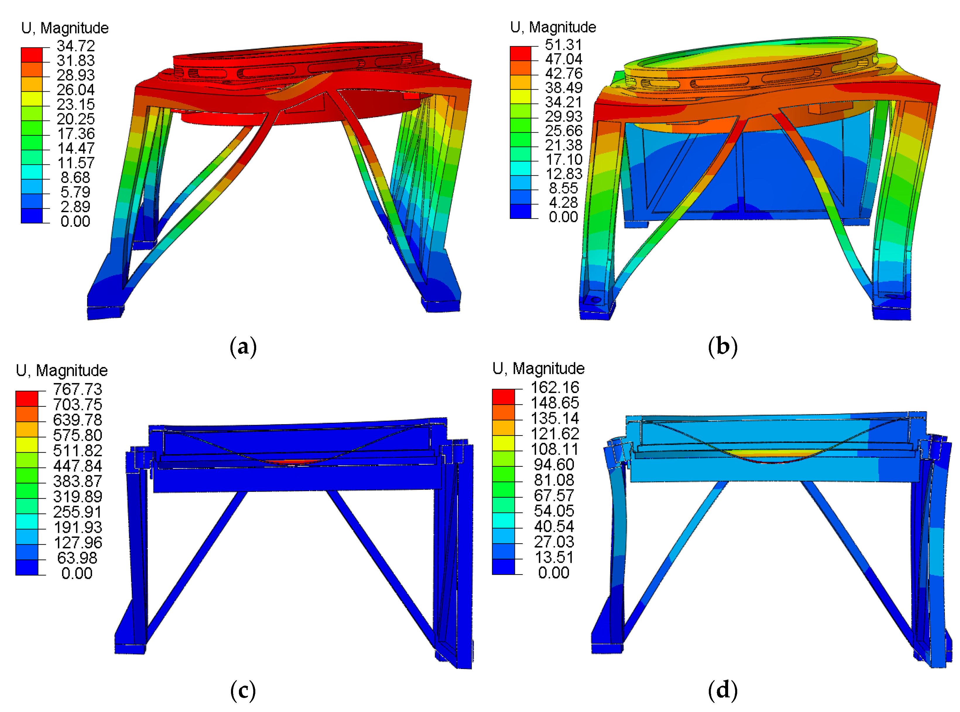
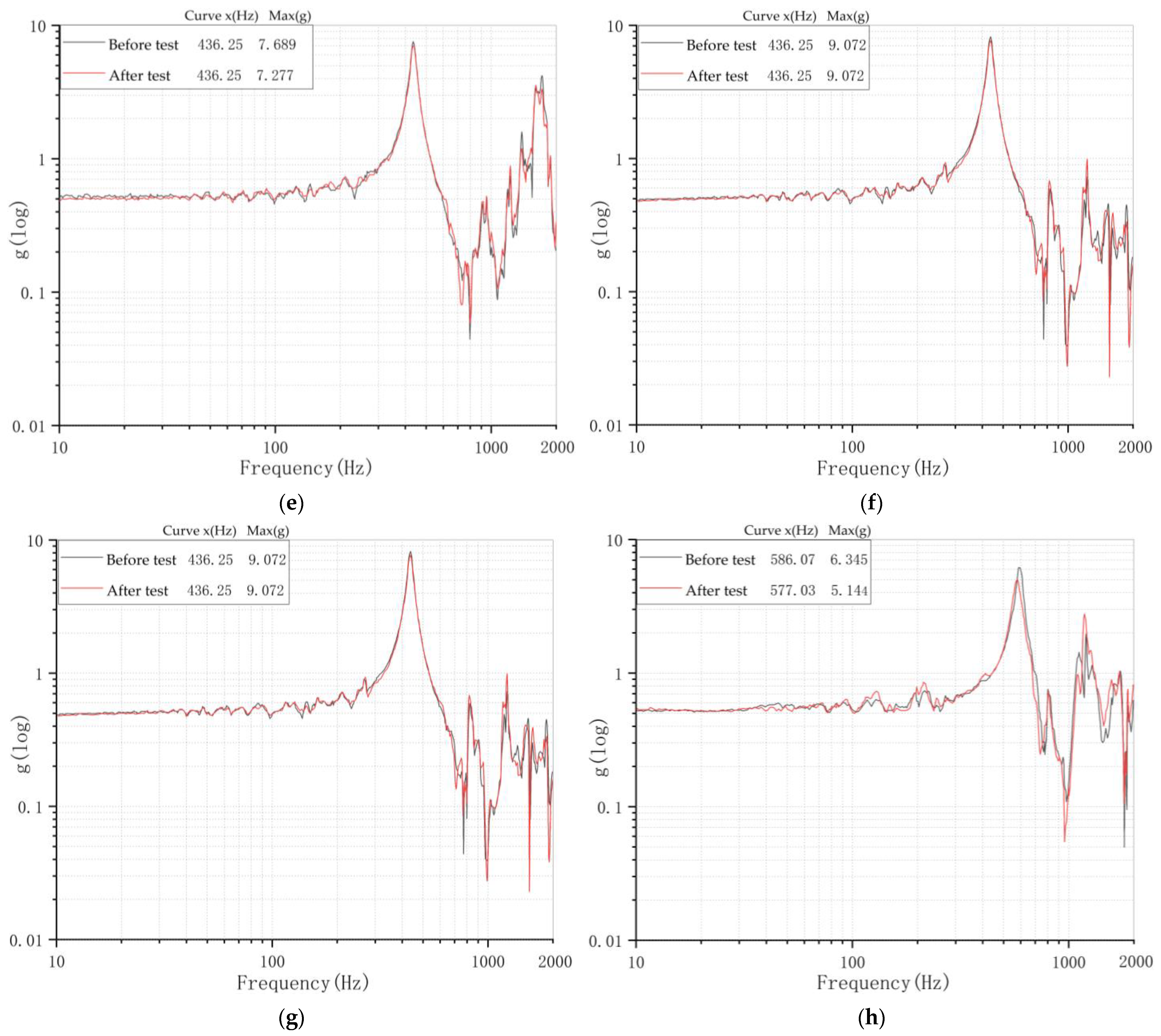
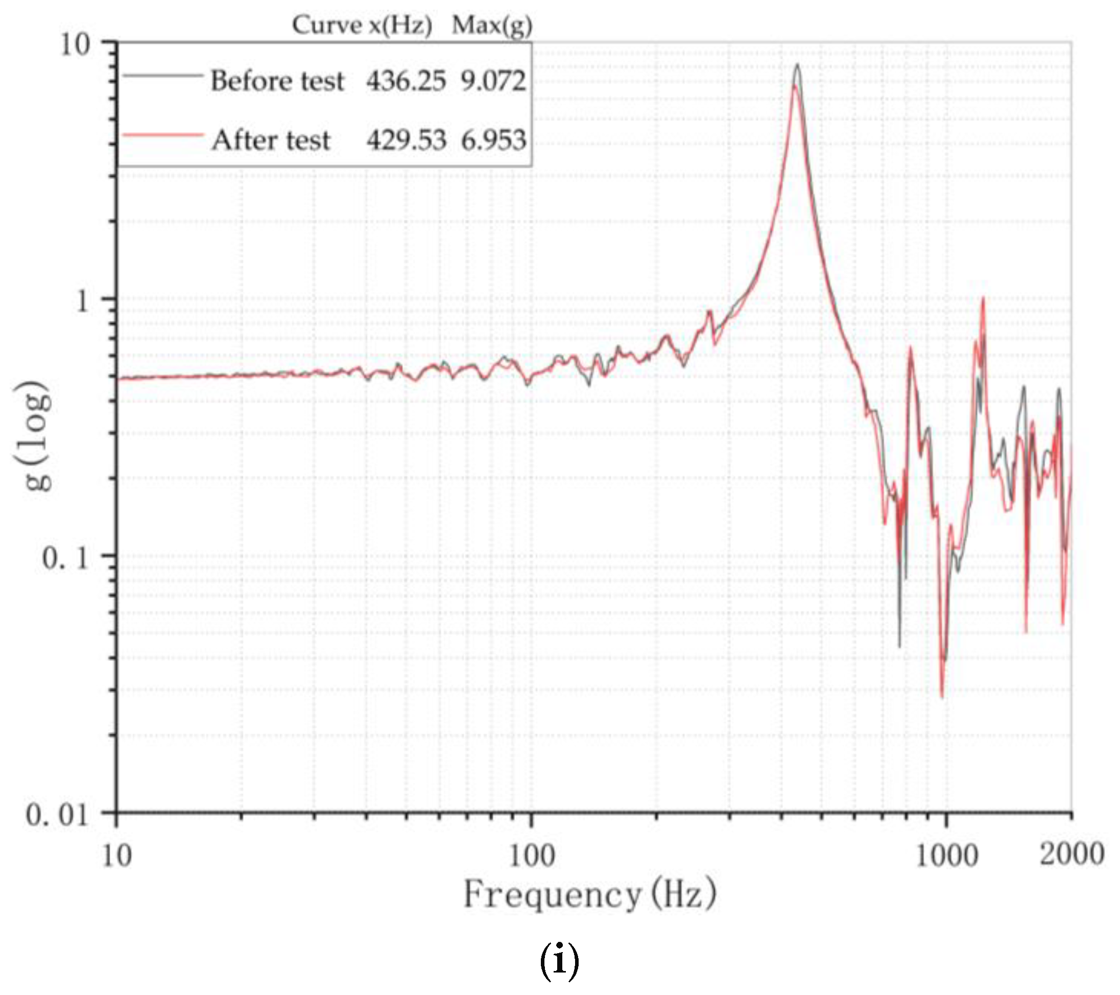
From the static strain cloud diagram, it can be found that the maximum displacement occurs at the center of the beryllium sheet of 15.48 μm, the maximum deformation is in the elastic deformation stage of the material, and the calculation result of the safety margin is dozens of times the specified standard.The sinusoidal characteristic sweep frequency test shows that the frequency of the first order main mode of the structure is 436.25 Hz, which is greater than the 100 Hz specified in the spacecraft. Through the sinusoidal characteristic frequency sweep before and after the mechanical vibration test, it is concluded that the first order frequency change in X, Y and Z directions of the structure is not more than the 5% specified for the spacecraft, which shows that the structure is not damaged under the mechanical vibration test. From the results discussed above, the stiffness and strength of the structure designed in this paper meet the mission requirements.

(2)

The empirical value of 0.03 adopted in the finite element calculation is deviated from the actual value. The finite element model is modified using the damping value calculated from the vibration test and half-power bandwidth method. The modified calculation results are in high agreement with the experimental values, which provides a damping reference value for the subsequent finite element calculation.

(3)

The comparison between modal analysis and sinusoidal characteristic sweep frequency test shows that the first order frequency error in each direction is within the allowable error range of 10% in the engineering analysis. The first order frequency is 420.25 Hz, which meets the requirement that the product must be greater than 100 Hz.

References

1. Frontera, F.; Costa, E.; Fiume, D.D.; Feroci, M.; Nicastro, L.; Orlandini, M.; Palazzi, E.; Zavattini, G. The high energy instrument PDS on-board the BeppoSAX X-ray astronomy satellite. Astron. Astrophys. Suppl. Ser. 1997, 122, 357–369. [Google Scholar] [CrossRef] [Green Version]
2. Matsuoka, M.; Kawai, N.; Yoshida, A.; Tamagawa, T.; Torii, K.; Shirasaki, Y.; Ricker, G.; Doty, J.; Vanderspek, R.; Crew, G.; et al. The gamma-ray burst alert system and the results of HETE-2. Balt. Astron. 2004, 13, 201–206. [Google Scholar]
3. Tavani, M.; Barbiellini, G.; Argan, A.; Auricchio, N.; Bernabeo, A.; Bulgarelli, A.; Caraveo, P.A.; Celesti, E.; Chen, A.W.; Cocco, V.; et al. The AGILE instrument. In Proceedings of the Conference on X-ray and Gamma-ray Telescopes and Instruments for Astronomy, Waikoloa, HI, USA, 24–28 August 2003; pp. 1151–1162. [Google Scholar]
4. Barbiellini, G.; Tavani, M.; Argan, A.; Auricchio, N.; Caraveo, P.; Chen, A.; Cocco, V.; Costa, E.; Di Cocco, G.; Fedel, G.; et al. The AGILE scientific instrument. In Proceedings of the Gamma-ray Astrophysics 2001 Symposium, Baltimore, MD, USA, 4–6 April 2001; pp. 774–778. [Google Scholar]
5. Tavani, M.; Barbiellini, G.; Caraveo, P.; Cocco, V.; Costa, E.; Di Cocco, G.; Labanti, C.; Longo, F.; Mereghetti, S.; Morselli, A.; et al. The AGILE contribution to GRBs studies. Astron. Astrophys. Suppl. Ser. 1999, 138, 569–570. [Google Scholar] [CrossRef]
6. Vercellone, S.; Chen, A.W.; Cocco, V.; Feroci, M.; Galli, M.; Giuliani, A.; Lapshov, I.Y.; Lipari, P.; Longo, F.; Mereghetti, S.; et al. Imaging of high energy sources with AGILE. AIP Conf. Proc. 2001, 587, 764–768. [Google Scholar]
7. Bhat, P.N.; Meegan, C.A.; Lichti, G.G.; Briggs, A.S.; Connaughton, V.; Diehl, R.; Fishman, G.J.; Greiner, J.; Kippen, R.M.; Kouveliotou, C.; et al. The Fermi Gamma-ray Burst Monitor Instrument. In Proceedings of the 6th Huntsville Symposium on Gamma-Ray Burst, Huntsville, AL, USA, 20–23 October 2009; p. 34. [Google Scholar]
8. Fangjun, L.; Shuangnan, Z. The Hard X-ray Modulation Telescope—China’s first X-ray astronomical satellite. Physics 2017, 46, 341–347. [Google Scholar]
9. YongWei, D.; BoBing, W.; Li, Y.; Zhang, Y.; Zhang, S. SVOM gamma ray monitor. Sci. China-Phys. Mech. Astron. 2010, 53, 40–42. [Google Scholar]
10. Wen, J.; Long, X.; Zheng, X.; An, Y.; Cai, Z.; Cang, J.; Che, Y.; Chen, C.; Chen, L.; Chen, Q. GRID: A student project to monitor the transient gamma-ray sky in the multi-messenger astronomy era. Exp. Astron. 2019, 48, 77–95. [Google Scholar] [CrossRef] [Green Version]
11. Tajima, H.; Watanabe, S.; Fukazawa, Y.; Blandford, R.D.; Enoto, T.; Goldwurm, A.; Hagino, K.; Hayashi, K.; Ichinohe, Y.; Kataoka, J. Design and performance of Soft Gamma-ray Detector onboard the Hitomi (ASTRO-H) satellite. J. Astron. Telesc. Instrum. Syst. 2018, 4, 021411. [Google Scholar] [CrossRef] [Green Version]
12. Frank, J.; Beitler, C.; Pietschner, D.; Strecker, R.; Antonelli, V.; Plattner, M.; Meidinger, N. Structural Analysis of Athena WFI Large Detector Array. In Proceedings of the SPIE Astronomical Telescopes + Instrumentation Conference, Los Angeles, CA, USA, 14–18 December 2021; Volume 11444. [Google Scholar]
13. Mangan, J.; Murphy, D.; Dunwoody, R.; Ulyanov, A.; Thompson, J.; Javaid, U.; O’Toole, C.; Doyle, M.; Emam, M.; Erkal, J.; et al. The environmental test campaign of GMOD: A novel gamma-ray detector. In Proceedings of the International Conference on Space Optics, Antibes, France, 30 March–2 April 2021; Volume 11852. [Google Scholar]
14. Liu, R.; Zhu, C.; Chen, W.; He, T.; Zhang, A.M.; Xu, Y.P.; Yu, J.P.; Zhu, Z.C.; Zhang, S.N.; Lu, F.J. Mechanical design and analysis of the eXTP satellite. In Proceedings of the SPIE Astronomical Telescopes + Instrumentation Conference, Los Angeles, CA, USA, 14–18 December 2021; Volume 11444. [Google Scholar]
15. Zins; John, W. Structural Analysis of the Space Telescope Wide-Field/Planetary Camera (Wf/Pc). In Proceedings of the OE LASE’87 and EO Imaging Symposium, Los Angeles, CA, USA, 12–16 January 1987; Volume 0748. [Google Scholar]
16. Jurcevich, B.; Bruner, M.; Gowen, K. Structural mechanics of the solar-A soft X-ray telescope. Design of optical instruments. In Proceedings of the Meeting, Orlando, FL, USA, 22–24 April 1992; Volume 1690. [Google Scholar]
17. Xue, Y.; Chen, Z.; Zhixing, L.; Ge, J.; Longhui, L.; Weimin, Y.; Shuangnan, Z. The Finite Element Analysis Modeling of Micro Pore Optic Plate. In Proceedings of the SPIE Astronomical Telescopes + Instrumentation Conference, Austin, TX, USA, 10–15 June 2018; Volume 10699. [Google Scholar]
18. McClelland, R.; Carnahan, T.; Choi, M.; Robinson, D.; Saha, T. Preliminary design of the International X-ray Observatory flight mirror assembly. In Proceedings of the SPIE Optical Engineering + Applications Conference, San Diego, CA, USA, 2–6 August 2009; Volume 7437. [Google Scholar]
19. McClelland, R.; Carnahan, T.; Robinson, D.; Zhang, W. Design and analysis of the International X-Ray Observatory mirror modules. In Proceedings of the SPIE Astronomical Telescopes + Instrumentation Conference, San Diego, CA, USA, 27 June–2 July 2010; Volume 7732. [Google Scholar]
20. McClelland, R.; Powell, C.; Saha, T.; Zhang, W. Design and analysis of mirror modules for IXO and beyond. In Proceedings of the SPIE Optical Engineering + Applications Conference, San Diego, CA, USA, 21–25 August 2011; Volume 8147. [Google Scholar]
21. Jimenez-Martinez, M.; Alfaro-Ponce, M. Effects of synthetic data applied to artificial neural networks for fatigue life prediction in nodular cast iron. J. Braz. Soc. Mech. Sci. Eng. 2021, 43, 10. [Google Scholar] [CrossRef]
22. Yang, Q.W.; Sun, B.X.; Lu, C. An improved spectral decomposition flexibility perturbation method for finite element model updating. Adv. Mech. Eng. 2018, 10, 1–11. [Google Scholar] [CrossRef]
23. Jifeng, D.; Zengyao, H.; Xingrui, M. Research evolution on the test verification of spacecraft dynamic model. Adv. Mech. 2012, 42, 395–405. [Google Scholar]
24. Jun-Yao, L.; Song, G.; Shan-bo, C. Mechanical Analysis of Microsatellite Structure Design Based on Moon Jellyfish. Comput. Simul. 2021, 38, 32–36.74. [Google Scholar]
25. Chao-bo, L.; Jing-jun, L.; Zhen-hai, Z. Simplified Model and Response Analysis for Crankshaft of Air Compressor. In Proceedings of the 4th International Conference on Advanced Materials, Mechanics and Structural Engineering (AMMSE), Tianjin, China, 22–24 September 2017; Volume 269. [Google Scholar]
26. Fulong, Z. The Structural Finite Element Analysis of the Mirror Module of eXTP-SFA/PFA; Institute of High Energy Physics Chinese Academy of Sciences: Beijing, China, 2021. [Google Scholar]
27. Naito, T.; Tsuboi, H. A simplification method for reflective and rotational symmetry model in electromagnetic field analysis. IEEE Trans. Magn. 2001, 37, 3554–3557. [Google Scholar] [CrossRef]
28. Hjelmervik, J.M.; Leon, J.-C. Simplification of FEM-Models on Cell BE. In Proceedings of the 7th International Conference on Mathematical Methods for Curves and Surfaces, Tonsberg, Norway, 26 June–1 July 2008; p. 261. [Google Scholar]
29. Langer, P.; Jelich, C.; Guist, C.; Peplow, A.; Marburg, S. Simplification of Complex Structural Dynamic Models: A Case Study Related to a Cantilever Beam and a Large Mass Attachment. Appl. Sci. 2021, 11, 5428. [Google Scholar] [CrossRef]
30. Yanqing, B.; Sankaran, M. Diagnosis of interior damage with a convolutional neural network using simulation and measurement data. Struct. Health Monit.-Int. J. 2022, 21, 2312–2328. [Google Scholar]
31. Cheng, D. Mechanical Design Handbook, 5th ed.; Chemical Industry Publishing House: Beijing, China, 2007; pp. 6–10. [Google Scholar]
32. Yuan, J. Satellite Structure Design and Analysis, 1st ed.; China Aerospace Publishing House: Beijing, China, 2004; Volume 1, pp. 163–203. [Google Scholar]
33. Zhao, X.; Zhao, C.; Li, J.; Guan, Y.; Chen, S.; Zhang, L. Research on Design, Simulation, and Experiment of Separation Mechanism for Micro-Nano Satellites. Appl. Sci. 2022, 12, 5997. [Google Scholar] [CrossRef]
34. Wang, J.; Li, T.; Zhao, H.; Ren, Q.; Zong, Y.; Liu, Q.; Fan, X. Dynamic Simulation and Vibration Test of the Active Potential Controller. In Proceedings of the 5th Asia Conference on Mechanical Engineering and Aerospace Engineering (MEAE), Wuhan, China, 1–3 June 2019; Volume 288. [Google Scholar]
35. Jun, Z.; Yong, C.; ZhiYi, Z.; Hongxing, H. Research on the Random Vibration Test of the Satellite. J. Mech. Strength 2006, 28, 16–19. [Google Scholar]
36. Guo-bin, M. Random Vibration Response Prediction of Some Spacecraft Attitude-Control Thruster Set. Aerospace 2007, 24, 54–57. [Google Scholar]
37. Mahamdi, A.; Benkouda, S.; Aris, S.; Denidni, T.A. Resonant Frequency and Bandwidth of Superconducting Microstrip Antenna Fed through a Slot Cut into the Ground Plane. Electronics 2021, 10, 147. [Google Scholar] [CrossRef]
Figure 1. Comparison of the traditional and novel GRM: (a) Novel GRM. (b) Traditional gamma-ray detector.
Applsci 12 11025 g001
Figure 2. GRM payload: (a) Assembly of bracket for radiant cooling plate. (b) Assembly of GRM payload.
Applsci 12 11025 g002
Figure 3. Finite element model.
Applsci 12 11025 g003
Figure 4. Vibration testing site: (a) X-axis direction. (b) Y-axis direction. (c) Z-axis direction.
Applsci 12 11025 g004
Figure 5. Finite element analysis boundary conditions.
Applsci 12 11025 g005
Figure 6. Layout of mechanical measurement points.
Applsci 12 11025 g006
Figure 7. Stress and strain cloud diagram of the novel GRM parts: (a) Overall stress and strain cloud diagram of the novel GRM. (b) Stress and strain cloud diagram of the beryllium sheet. (c) Stress and strain cloud diagram of the quartz. (d) Stress and strain cloud diagram of the structural adhesive.
Applsci 12 11025 g007aApplsci 12 11025 g007b
Figure 8. Mathematical model of structural adhesive shear stress: (a) column coordinate system; and (b) schematic diagram of shear stress in column coordinate system.
Applsci 12 11025 g008
Figure 9. First 4 orders of vibration and frequency: (a) First order Y-directional vibration frequency is 420.25 Hz. (b) Second order Z-directional vibration frequency is 615.66 Hz. (c) Third order local vibration frequency is 618.68 Hz. (d) Fourth order X-directional vibration frequency is 732.34 Hz.
Applsci 12 11025 g009
Figure 10. Plots of characteristic swept spectral lines before and after the sinusoidal characteristic sweep frequency test in X, Y, and Z directions for each measurement point: (a) Measurement point 1 in X-direction. (b) Measurement point 2 in X-direction. (c) Measurement point 3 in X-direction. (d) Measurement point 1 in Y-direction. (e) Measurement point 2 in Y-direction. (f) Measurement point 3 in Y-direction. (g) Measurement point 1 in Z-direction. (h) Measurement point 2 in Z-direction. (i) Measurement point 3 in Z-direction.
Applsci 12 11025 g010aApplsci 12 11025 g010bApplsci 12 11025 g010c
Figure 11. Comparison of acceleration response curve between theoretical analysis and experimental test: (a) Acceleration response curve of theoretical analysis in X-directional. (b) Acceleration response curve of experimental test in X-directional. (c) Acceleration response curve of theoretical analysis in Y-direction. (d) Acceleration response curve of experimental test in Y-direction. (e) Acceleration response curve of theoretical analysis in Z-directional. (f) Acceleration response curve of experimental test in Z-directional.
Applsci 12 11025 g011aApplsci 12 11025 g011b
Figure 12. Comparison of theoretical analysis and experimental test PSD response curves: (a) X-directional PSD response curve of theoretical analysis. (b) X-directional PSD response curve of experimental test. (c) Y-directional PSD response curve of theoretical analysis. (d) Y-directional PSD response curve of experimental test. (e) Z-directional PSD response curve of theoretical analysis. (f) Z-directional PSD response curve of experimental test.
Applsci 12 11025 g012aApplsci 12 11025 g012b
Figure 13. Sinusoidal characteristic sweep frequency map of measurement points before and after X, Y, Z random test: (a) Measurement point 1 in X-direction. (b) Measurement point 2 in X-direction. (c) Measurement point 3 in X-direction. (d) Measurement point 1 in Y-direction. (e) Measurement point 2 in Y-direction. (f) Measurement point 3 in Y-direction. (g) Measurement point 1 in Z-direction. (h) Measurement point 2 in Z-direction. (i) Measurement point 3 in Z-direction.
Applsci 12 11025 g013aApplsci 12 11025 g013bApplsci 12 11025 g013c
Figure 14. Performance test before and after mechanical vibration test: (a) Performance test site. (b) Result of performance test.
Applsci 12 11025 g014