Article

Fault Diagnosis Algorithm of Beam Pumping Unit Based on Transfer Learning and DenseNet Model

1
School of Mechanical Science and Engineering, Northeast Petroleum University, Daqing 163000, China
2
College of Mechanical and Electrical Engineering, Wenzhou University, Wenzhou 325000, China
3
Geophysical Institute, China Petroleum Exploration and Development Research Institute, Beijing 100107, China
*
Author to whom correspondence should be addressed.
Appl. Sci. 2022, 12(21), 11091; https://doi.org/10.3390/app122111091
Submission received: 18 October 2022 / Revised: 27 October 2022 / Accepted: 28 October 2022 / Published: 1 November 2022
(This article belongs to the Section Computing and Artificial Intelligence)

Abstract

:
The difficulty of collecting fault data samples is one of the application problems of the deep learning method in fault diagnosis of mechanical production; the second is that when the depth of the learning network increases, the network accuracy is saturated or even decreased. Therefore, based on the deep learning algorithm and the DenseNet model, this paper establishes a fault diagnosis model for the beam pumping unit through the transfer learning method. The model uses the global pooling layer as the classifier. The model is used to classify and test various working conditions such as wax deposition, pump leakage, insufficient liquid supply, and pump leakage in oil wells. The results show that the model can obtain a classification model with high accuracy by learning a limited number of sample data; in the case of uneven data samples, the model can also basically complete the task classification task accurately. Through the evaluation of the test set, the model has an average accuracy of more than 95% in identifying various working conditions.

1. Preface

Oil, as a nonrenewable energy source, is increasingly important to the development of modern society and the economy. Most of the authors’ country’s oil fields have entered the middle and late stages of production, and many oil wells have more than 95% water content, and problems such as eccentric wear, corrosion, and scaling are serious. By 2018, CNPC had 184,600 oil wells in service, of which 90% were beam pumping wells. Twenty-five per cent of oil wells had a pump inspection period of less than 300 days, of which 4237 wells had more than 3 high-frequency pump inspections, accounting for 17% of the operation volume. The operation cost is 700 million yuan, affecting the output of 250,000 tons.
The beam pumping unit has the characteristics of field operation, large quantity, scattered location, harsh environment, and complex working conditions, and it is very difficult to manage and monitor. To diagnose and discover various abnormal working conditions of pumping wells as early as possible, petroleum engineering scientists have studied various fault diagnosis techniques, such as expert system fault diagnosis, fuzzy fault diagnosis, neural network fault diagnosis, and deep learning fault diagnosis.
The most widely used method to analyze the performance and fault diagnosis of pumping wells is by means of a hanging nodes indicator diagram. The hanging node indicator diagram is a closed curve which can reflect the downhole condition of the oil well based on the shape, and different working conditions have different curve characteristics. Artificial perception methods are time-consuming, labor-intensive, and error-prone. Therefore, an automated diagnosis method is needed to improve the efficiency of manual maintenance. In 1988, after visiting many famous experts, Derek et al. [1] developed an expert system for fault diagnosis of rod pumping wells. They achieved this by converting the indicator diagram on the ground into a downhole indicator diagram, then comparing it with the standard indicator diagram to determine the type of fault. However, the weakness of the system is that it relies too much on the domain knowledge of experts in the petroleum industry. In 1990, Rogers et al. [2] introduced the theory of artificial neural networks into the indicator diagram recognition domain. They applied the error back propagation learning algorithm to train the neural network and were able to identify 15 types of indicator diagrams. The neural network method has shown good application potential in this kind of problem. However, due to the relatively simple structure of the neural network it uses, the effect of using it is not ideal. In 1994, Nazi et al. [3] used a three-layer hybrid feedforward network model of the sinusoidal hidden layer perceptron algorithm and the sigmoid output layer perceptron algorithm, which completed the classification task of 11 fault types through the training of 167 dynamometer diagrams. In 2016, Wen Bilong et al. [4] used a fuzzy neural network to solve the problem of oil pumping unit fault diagnosis. The fuzzy theory diagnosis method needs to establish a membership function first, but the membership function is artificially constructed and contains subjective factors. In addition, there are certain requirements for the selection of characteristic elements, which limits the application of the fuzzy neural network method.
The fault diagnosis method of artificial perception pattern has the problems of high cost, long time, inconsistent analysis results, and being error-prone. Traditional pattern recognition technology requires a lot of domain expert knowledge and expression reasoning mechanisms, which are difficult to popularize and use. The machine learning diagnosis method can extract characteristic information to analyze and evaluate the system only by analyzing the historical monitoring data. The application data model replaces the accurate complex system model, which has good generalization and is easy to apply.
In recent years, machine learning has been widely used in the field of fault diagnosis. For example, Rauber et al. [5] designed the original feature vector based on 26 statistical parameters, 72 envelope characteristics, and 32 wavelet envelope characteristics, and then used support vector machines (Support Vector Machine, SVM) to identify the bearing faults. Chine et al. [6] calculated several characteristic parameters and used an artificial neural network for fault diagnosis of the photovoltaic system. Wijayasekara et al. [7] proposed a novel fuzzy neural data fusion engine for online monitoring and diagnosis. The above methods have achieved certain results, but due to the limitations of artificial feature extraction, and the fact that there is no authoritative theory to guide the design method of feature functions, such methods are difficult to popularize and use.
Deep learning, one of the branches of machine learning, is valued because it can extract features from data automatically and reduce the uncertainty in the process of artificial data extraction effectively. For example, Chen et al. [8] fused the vibration data in the horizontal and vertical directions into a two-dimensional matrix and proposed a deep CNN to identify gearbox operating conditions. Janssens et al. [9] identified four rotating mechanical states by a two-dimensional CNN model. Using the discrete Fourier transform of two vibration signals as input to a CNN, faults in rotating machinery are classified and compared with artificially designed faults. The results show that the CNN-based method outperforms traditional methods and does not require any artificial feature extraction with domain expertise.
In recent years, fault diagnosis methods based on deep learning have received attention in the petroleum industry. Zhao et al. [10] proposed a data-based CNN method and an image-based CNN method for fault diagnosis of a rod oil pumping system and compared them with traditional machine learning algorithms. The results show that the CNN-based method is superior to the traditional method, as it does not need to extract any artificial characteristics of experts in the field. Wang et al. [11] proposed a 14-layer CNN diagnostic model based on big data deep learning to identify the working conditions of rod pumping wells. In 2020, Cheng et al. [12] used a combination of transfer learning and SVM to identify operating conditions in indicator diagrams automatically. This kind of method solves the problem that feature extraction is more difficult and has no guaranteed effect. However, the above research is based on the laboratory or a few working conditions, and the various types of data are processed uniformly, which is inconsistent with the actual work situation, which leads to the following problems in practical applications:
(a) Most of the mechanical fault diagnosis studies are based on balanced data sets, ignoring the fact that the amount of data in different working conditions in the actual production process are often highly unbalanced. In the actual recorded data, as shown in Figure 1, the number of each working condition type is not uniform. In practical applications, mechanical equipment is in a normal state during most of the operation stages, and failures rarely occur during operation [13]. In the actual working environment, there are many kinds of faults, and it is difficult to provide sufficient samples. The rod pump model may automatically ignore some working conditions affecting the actual use.
(b) Most of the sample research data for mechanical fault diagnosis come from the experimental environment or from a small amount of equipment operation data. Because of the similarity of the sample data, the classification results are good, but the generalization is poor. Therefore, the performance of the fault diagnosis model is affected in actual use.
To solve the problems of insufficient training data and uneven distribution of the deep learning, the fault diagnosis method for sucker rod pumps, and serious performance degradation of the deep model is seen when working conditions change. This paper puts forward an intelligent fault diagnosis model for the sucker rod pump based on transfer learning and the DenseNet model. First, transfer the pretraining model which is established according to the DenseNet image recognition model structure to a new neural network model, and using the actual working conditions of the artificial perception data for preliminary training. Second, fine-tune the preliminary training achieves a certain effect and further obtains the artificial perception classification model; finally, the working condition diagnosis is carried out according to the fault artificial perception classification model. This method can effectively avoid the problem of model fitting caused by the limitation of data type and quantity, and can also improve the problem that special working conditions cannot be effectively identified due to the uneven distribution of various samples. At the same time, this paper uses actual production data to test, and the results show that the model established by this method can meet the actual production requirements.

2. Fault Diagnosis Model and Application Method

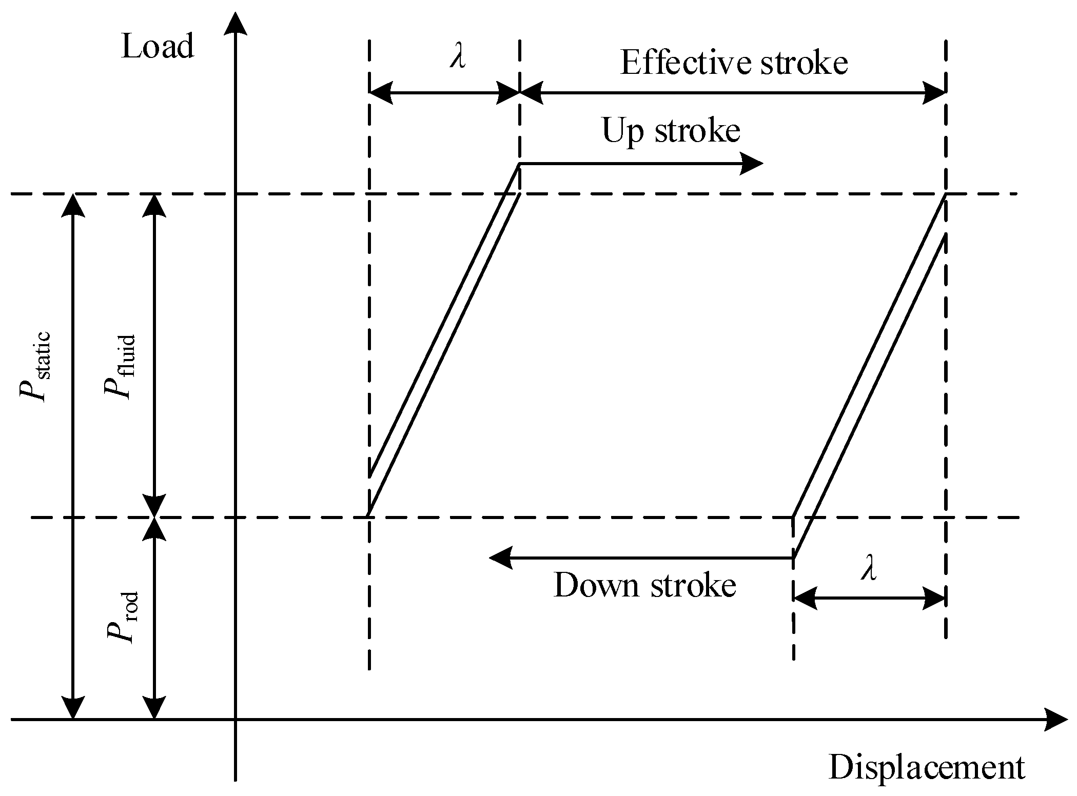
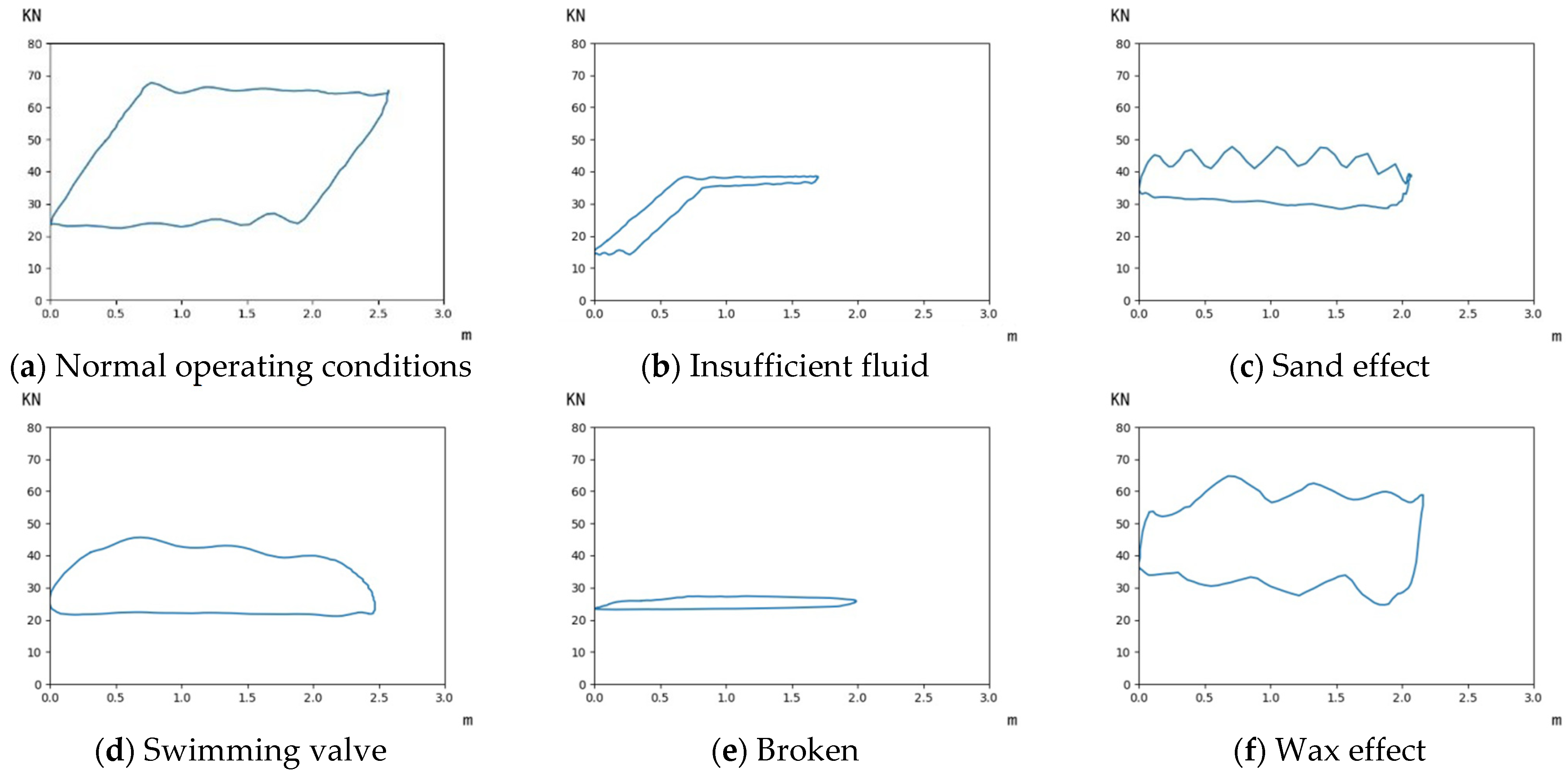
2.1. Sucker Rod Pump Fault Diagnosis

The polished rod indicator diagram is often used to judge downhole working conditions. The ground polished rod dynamometer can draw the relationship between the load and displacement of the polished rod through the test data, that is, the polished rod indicator diagram. The fault type of the oil well can be judged by calculating and analyzing the indicator diagram. Researchers in various countries expand the scope of interpretation by improving the precision of the dynamometer and the interpretation method of indicator diagrams. As the main means to judge the sucker rod pump’s fault, the optical rod dynamometer has been widely used until today because of its advantages of convenient operation and use. Figure 2 shows the theoretical indicator diagram under static load.
In Figure 2, λ is the stroke loss; Pliquid is the gravity of the liquid column above the pump; Prod is the gravity of the sucker rod in the liquid; Pstatic is the static load on the polished rod. The indicator diagram is surrounded by closed line segments, and the area represents the work done by the pumping unit in one reciprocating motion. The dynamometer diagram of the pumping unit is close to a parallelogram under normal working conditions. In the production operation, it is different to compute due to the complex underground working environment of the pumping unit. In addition to the manufacturing and installation of the pumping unit itself, downhole geological conditions such as fluid, sand inclusions, liquid gas, and other factors can also cause the indicator diagram to have a variety of different shapes.
A total of 15 fault types are studied in this paper: plunger up bump, plunger down bump, insufficient fluid supply, double vale loss, fixed vale loss, broken rod, normal operating conditions, gas effect, pump leakage, plunger coming out, swimming vale loss, sand effect, heavy oil effect, wax effect, pump and eject. Figure 3 is an indicator diagram of six common faults, where the horizontal axis represents the displacement and the vertical axis represents the load.

2.2. Fault Diagnosis Model

2.2.1. Convolutional Neural Network and Transfer Learning

The convolutional neural network is one of the classic algorithms of deep learning, that is, a kind of feedforward neural network that includes convolutional computation and has deep structure. The convolutional neural network is constructed by imitating biological visual perception, and its convolution layer can describe the image features with a small amount of computation, which enables it to have a stable operation effect and means it does not need to carry out additional feature engineering features [14]. A convolutional neural network consists of an input layer, a hidden layer, and an output layer. After the data are filtered, the input layer preprocesses the filtered data and converts all data into a unified format, the preprocessed images are input to the convolutional layer and pooling layer for feature extraction and computational analysis, and the images to be classified are converted into feature images. Through full connection layer matching, the final output is reached the target value. The main execution flow is shown in Figure 4 [15]. The input layer of the convolutional neural network can receive arrays from one to four dimensions depending on the structure. Before input of the learning data into the hidden layer, the data should be normalized to improve the accuracy and efficiency of the algorithm.
The hidden layer of a convolutional neural network algorithm usually consists of three structures: convolutional layer, pooling layer, and fully connected layer. We identify the two-dimensional convolution function of the image as Equation (1) [16]:
S = X × W = i , j = 1 m × n x ij × w ij
where:
  • S—characteristic coefficient;
  • X—input matrix;
  • W—convolution kernel matrix;
  • (i, j)—the position of the variable in the feature matrix;
  • (m, n)—the position of the convolution kernel element.
The convolutional layer contains multiple convolution kernels, which are similar to neurons in a feedforward neural network. The parameters of the convolution layer include the size, step size, and filling method of the convolution kernel. These three factors jointly determine the size of the output feature graph of the convolutional layer. The convolutional layer contains an excitation function to help it express complex features. After feature extraction in the convolutional layer, feature selection and filtering are carried out in the convolutional layer. Through the preset pooling function, the result of a single point in the feature map is replaced by its neighboring area feature map statistics. The pooling function is expressed as Equation (2) [17,18]:
A ( i , j ) = [ x = 1 f y = 1 f A k l ( s 0 i + x , s 0 j + y ) p ] 1 p
where:
  • s 0 —step length;
  • A—output value;
  • f—size of pooling layer;
  • p—optional coefficient, when p = 1, the value of A(i, j) is denoted as L1(A), called mean pooling; when p = ∞, the value of A(i, j) is denoted as L(A), called maximum pooling;
  • μ —the random parameter is determined by the actual operation;
  • k value—calculated channel position;
  • l—calculate channel position.
The fully connected layer of the convolutional neural network is located at the end of the hidden layer of the convolutional neural network, which expands the feature graph into a vector and transmits it to the next layer through the activation function. The fully connected layer performs a nonlinear combination of the extracted features and uses the extracted high-order features for learning.
Transfer learning is a method in the field of big data, used to apply a known model to a new field and is often used in deep learning tasks in computer vision and natural language processing. The implementation process is to train the existing model as the basis of the new model to achieve the purpose of reducing the computing cost and speeding up the computing speed.
Transfer learning imitates the human visual system, making full use of prior knowledge from different but related domains when performing new tasks in a given domain and solving related cross-domain learning problems. In transfer learning, extracting representative information and applying it to a new task can effectively improve the computational efficiency of the new task model. For learning tasks with scarce feature data, transfer learning can retain existing features while learning new features to avoid feature extraction errors caused by insufficient samples.
In 2014, Bengio et al. [19] studied the transferability of each layer feature in deep learning. The experimental results are as follows: When deep learning is applied to image processing, the features extracted by the first layer are basically similar to the Gabor filter and color spots. In general, the first layer is not clearly related to the specific image dataset, while the last layer of the network is closely related to the selected dataset and its mission objectives. Bengio refers to the first layer of features as general features and the last layer as specific features, and summarizes them as follows:
  • Feature transfer can improve the generalization performance of the model, even when the target dataset is very large.
  • When the parameters are fixed and the number of layers increases, the transfer accuracy between two tasks with low similarity increases faster than that between two tasks with high similarity. The greater the difference between the two datasets, the worse the effect of feature transfer.
  • Migration is better than using random parameters in any task.
  • Initializing the network with migration parameters can still improve the generalization performance, even if the target task has been heavily tuned.
The above research shows that even if there is a lack of approximate data sets, or the data are transferred to different fields, the transfer learning method can still effectively improve the training effect of machine learning and improve the generalization performance of the model.

2.2.2. Neural Network Framework

To explore the effect of different neural network models on indicator diagram recognition, this paper intends to select different classification models to classify and test the actual data. This article uses the TensorFlow open-source machine learning platform to conduct dynamometer classification experiments. The model pretraining datasets selected in the control experiments are all ImageNet datasets.

3. Dynamometer Classification Model Based on the Transfer Learning Method

3.1. Data Preprocessing

Data preprocessing includes image size definition, sample labeling, sample training, batch classification, and sample normalization. The purpose of data preprocessing is to make the sample format consistent for easy calculation, while removing redundant information to reduce the amount of calculation
A total of 5053 sets of fault diagnosis data were collected in a well area in Daqing Oilfield, including 37 types of data including normal, plunger up bump, plunger down bump, insufficient fluid supply, pump leakage, broken rod, and gas effect. The production data are filtered according to the data type, and the types with less than 10 groups of production data of the same type are classified as the other, and there are 15 main fault types in actual production. After cleaning up the defective data (such as lost data, unexplained data, obvious errors, etc.), the remaining 3502 groups of valid data were classified and stored. Labels were assigned to 15 fault types, and their indexes and quantities are shown in Table 1.
The indicator diagram was drawn according to the data, and all JPG images were unified into 600 × 400 pixels with the same coordinate system. Of these, 20% were randomly selected as test set data and the remaining 80% as training set. After segmentation, the sequence of indicator diagram data is fully disordered, and the training data set is packaged. The indicator diagram data are normalized, as shown in Equation (3):
x i ^ = x i 225 127.5
where:
  • x i ^ —Represents the pixel value of i th pixel of the sample after normalization;
  • x i —The i th pixel value of the sample, the purpose is to classify all pixels as [−1, 1].
According to the statistical results of the number of each fault type in Table 1, the data amount of each type generated in actual production is not uniform, which does not meet the requirement of data amount equality in traditional machine learning. At the same time, the amount of data generated in actual production is often limited, and it needs to be accumulated for a period of time to meet the requirements of machine learning. Therefore, according to the characteristics of actual oil well production data, the transfer learning method is used to establish the recognition model.

3.2. Transfer Learning Model Based on DenseNet

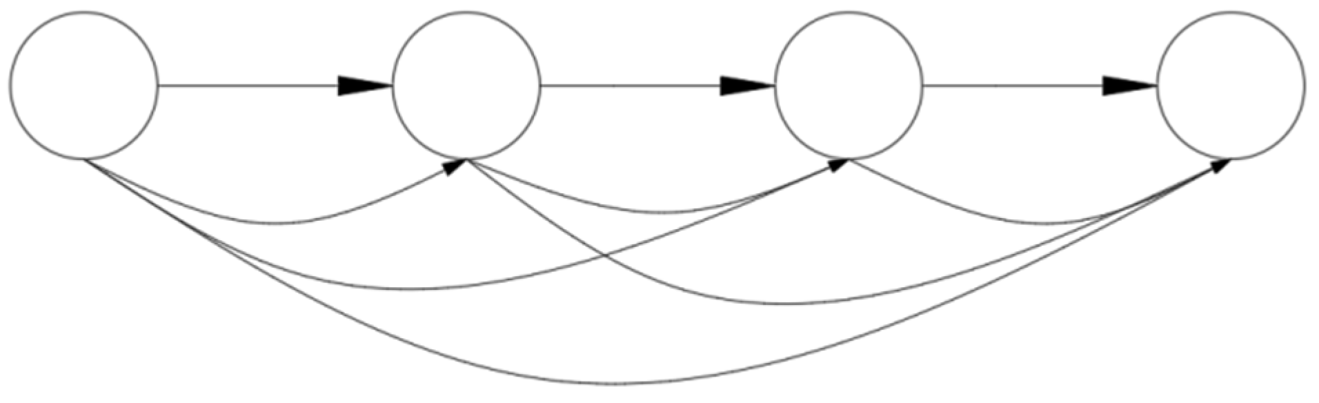
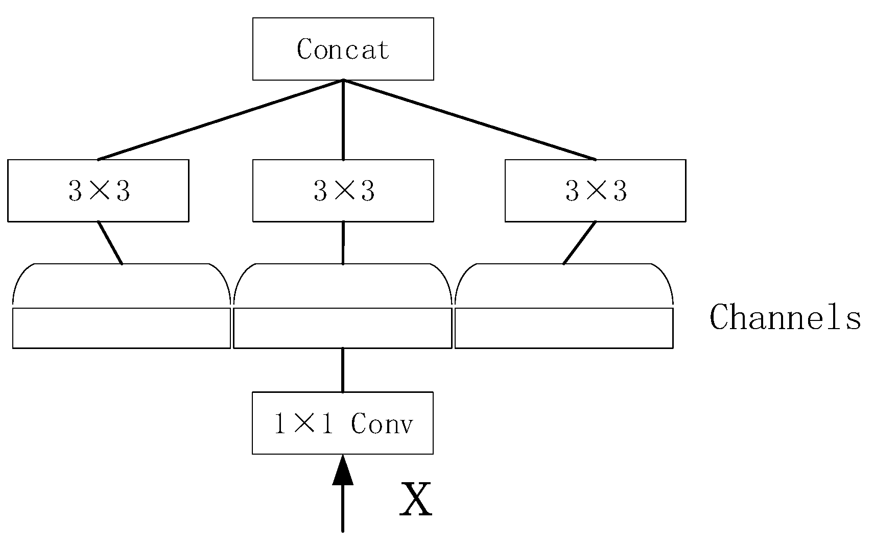
3.2.1. DenseNet Model Structure

Machine learning is a method to analyze data by generating models based on known data sets. The analysis of data features is essential in the process of building recognition models. When the feature information is insufficient, the recognition model cannot reach the ideal state. Too much feature information will lead to a high cost of calculation of the recognition model, which is not convenient for practical use. Therefore, whether the features extracted from the target image can be effectively utilized is one of the key factors affecting the classification effect of the model. The DenseNet model’s densely connected approach transmits signals from each layer to the bottom layer to maximize the use of effective features. As shown in Figure 5, compared with the traditional L-layer convolutional network with L connections, DenseNet has L ( L + 1 ) 2 connections in the L-layer convolutional network [17].
The network input at layer L is expressed as Equation (4):
x l = H l ( [ x 0 , x 1 , , x l 1 ] )
where:
  • x i ,     i = 0 , 1 , 2 , l 1 —Input parameters for each layer;
  • H l —is a compound function composed of Batch Normalization (BN), activation function (ReLU), pooling function, and convolution layer (Conv).
In the dense connection mode, each layer in the DenseNet model can receive all previous layer information, that is, feature propagation is strengthened, parameter reuse is realized, the number of parameters is reduced, and the calculation process is simplified.
This paper establishes the basic model of the DenseNet structure and retains the convolutional layer as the feature extraction structure after pretraining on ImageNet. The structure of each layer of the convolutional layer maintains the BN-ReLU-Conv in order to avoid gradient vanishing. Taking into account the characteristics of the indicator diagram image, the pooling layer structure adopts the average pooling function to maximize the retention of the overall data characteristics, such as in Equation (5):
L 1 ( A ) = x = 1 f y = 1 f A k l ( s 0 i + x , s 0 j + y )
To avoid overfitting, add the dropout function Equation (6) to the model:
r ( l ) ~ B e r n o u l l i ( p ) , y ~ ( l ) = r ( l ) × y ( l ) , f ( x ) = m a x ( 0 , x ) , y ( l + 1 ) = f ( w ( l + 1 ) × y ~ ( l ) + b l + 1 )
where:
  • Bernoulli function—r generates a vector r with Bernoulli distribution;
  • y ( l ) —the output value of the l-th layer;
  • w ( l + 1 ) —the weighted value of the neural network of the l + 1 th layer;
  • b l + 1 —the offset value;
  • p —determined by the number of neurons in the fully connected layer.
In the transfer process, this function can remove some weights in the layer, and the deleted weights will not disappear, but will also be reactivated by the use of the model. The main purpose of using this function is to simplify the calculation process and prevent overfitting caused by the overly complex model structure.
The model uses the loss function to evaluate the gap between the predicted model and the actual results and uses the cross-entropy loss to represent the loss. The function is as follows in Equation (7):
l = i = 1 K y i × ln ( p ( x j ) )
where:
  • l—the amount of loss;
  • K—the number of classifications;
  • y —the actual label, y = [ y 1 , , y i , y k ] ;
  • p ( x ) —the predicted label, p ( x ) = [ p ( x 1 ) , , p ( x j ) , , p ( x k ) ] .
Because cross-entropy can measure the difference between two probability distributions, this paper uses the cross-entropy function as the loss function to measure the difference between the true probability distribution and the predicted probability distribution. The smaller the cross-entropy value, the better the prediction effect of the obtained model.

3.2.2. Model Training Mechanism

To improve the learning effect, the hyperparameters in the transfer learning model based on the DenseNet model (hereinafter referred to as the dense connection model) are tested and adjusted. To train the dense connection model, we set the initial learning rate to be 0.1, 0.01, and 0.001 for testing, and ultimately obtain the best effect when the initial learning rate is 0.01. At this rate, the training speed of the dense connection model is better and the fluctuation is small.
One epoch means that a data set passes a neural network, and the learning time of the test run is 100 epochs. According to the image size, the structural complexity of the dense connection model, and the conditions of computing equipment, the size of a single data set is set to 32, that is, when there are 32 images in a single data set, the dense connection model has a better convergence speed.
Since the learning rate has a significant impact on the performance of the densely connected model, an adaptive learning rate optimization algorithm is adopted considering the possibility of other changes, except the initial learning rate setting and the learning rate changing with the number of trainings. The Adam optimization algorithm is used in the training of the dense connection model. The algorithm has the advantages of high computational efficiency and low memory usage, and is suitable for large-scale data when applied to nonconvex optimization problems. It is expressed as Equation (8):
m t = β 1 m t 1 + ( 1 β 1 ) g t v t = β 2 v t 1 + ( 1 β 2 ) g t 2 m ^ t = m t 1 β 1 t v ^ t = v t 1 β 2 t W t + 1 = W t η v ^ t + ϵ m ^ t
where:
  • m t and v t —the first-order momentum and second-order momentum;
  • β 1 and β 2 —usually take 0.9 and 0.999 for the power value;
  • W t —the parameters of the model in the t-th iteration;
  • g t —the gradient value of the loss function with respect to the parameter W in the t-th iteration;
  • ϵ —The minimal constant (usually takes its value to the 10−8 to avoid a zero denominator);
  • η —the initial learning rate.
Before training, the ImageNet dataset is used to load the structure to obtain a pretrained model, and then the training set for training and fine-tuning is loaded. The specific process is to freeze the saved basic model parameters and train the classifier. After the training results have stabilized, the frozen parameters are activated and fine-tuned with a lower learning rate.
For the recognition model based on the DenseNet model using the global pooling classifier, this paper uses two types of classifiers, the fully connected layer and the global pooling layer, respectively. Due to the limited number of training samples and the characteristics of the indicator diagrams, it is not necessary to use color adjustment or image inversion for data augmentation to increase training samples
After testing in the fully connected layer, the dropout layer parameter is 0.2, the L2 regularization is 0.0001, and the effect is better. At this time, the model can effectively avoid overfitting caused by too many parameters and ensure the training speed.

3.3. Training Results and Discussion

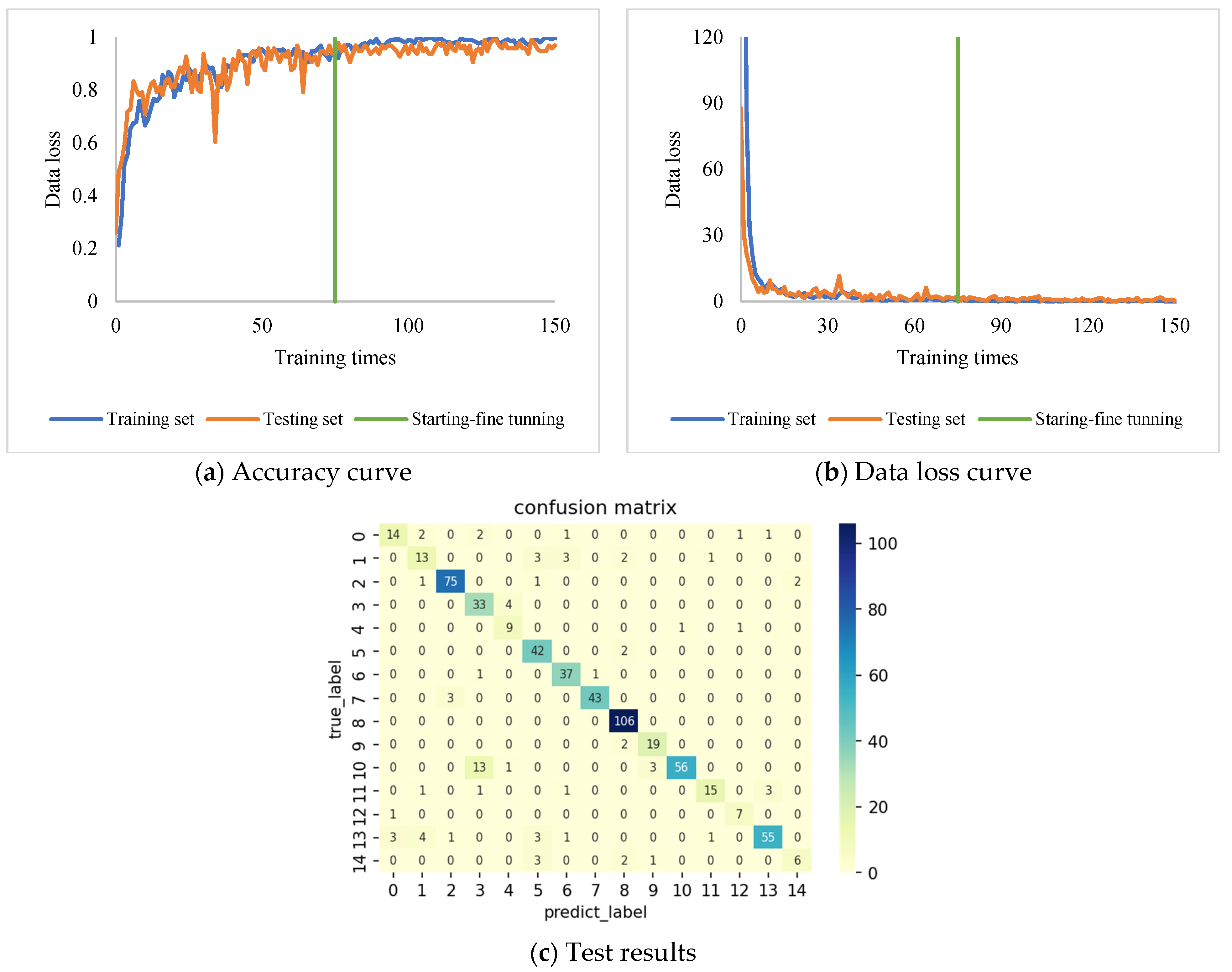
3.3.1. Training Results Based on Transfer Learning

This paper uses the TensorFlow machine learning development platform to conduct a DenseNet model-based transfer learning model indicator diagram classification experiment. The experimental environment is the NVIDIA Tesla T4 computing platform. The indicator diagram graph features are mainly composed of contour information, so this paper adopts global average pooling. The model was tested during the training set and test set, and Figure 6 records the output results of the training set and test set, respectively. The recognition accuracy of the test set is 96.9%, the output loss of the test set is 0.401, and the single training time of the model is 5.032 s.
The training results of the densely connected model using the global pooling layer classifier are shown in Figure 6. Figure 6a shows the development trend of the accuracy rate. Initially, the accuracy rate increased rapidly, but the upward trend quickly flattened and stabilized within the range of 80% to 90%; after 140 times of training, the dense connection model was thawed and fine-tuned, the accuracy rate had increased significantly, and the accuracy rate of the training set had stabilized above 99%
Figure 6b shows the data loss curve, the trend of which is basically the same as the accuracy curve. The data loss is relatively large at the beginning of training, but it will quickly drop to a stable range, and then the data loss will drop significantly after the model is thawed and fine-tuned. The pretraining set curve in Figure 6a is lower than the validation set curve, because the dropout layer randomly selects the parameters to freeze during the training process, and the curve appears after fine-tuning. The cross-training set accuracy improves rapidly.
The data loss curve in Figure 6b shows that the data loss of the validation set during training is unstable, showing a downward trend but fluctuating greatly, which affects the final accuracy. There were 747 indicator diagrams randomly selected which contain all the types of working conditions that were tested for classification. The results are shown in Figure 6c. It can be seen from Figure 6c that the model performs well under various types of working conditions and can meet the actual requirements, and various working conditions can achieve a high recognition rate.
To verify the classification effect of the dense connection model on the indicator diagram, the classification effects of the fully connected layer classifier and the global pooling classifier were compared under the same experimental conditions. The recognition accuracy of the test set is 96.9%, the output loss of the test set is 0.371, and the single training time of the model is 7.038 s
The model training results of the densely connected model using the fully connected layer classifier are shown in Figure 7. It can be seen from Figure 7a,b that the initial accuracy rate increases rapidly, and the loss function decreases rapidly, indicating that the transfer learning model can quickly adapt to new tasks. The accuracy of the dense connection model based on the full connection layer increased with the increase of training time, and the model was thawed by fine-tuning after the increasing trend was flat, and the model accuracy increased as a whole. After 100 times of training, the accuracy curve of the training set basically tends to be flat and can be maintained above 98%; the curve of the validation set and the curve of the training set have a similar growth trend, and there is a curve crossing phenomenon, indicating that the neural network is not appear to be overfitting.
After training, pictures containing all types of working conditions are randomly selected from the test set, for a total of 747 pictures, and are classified and tested to obtain Figure 7c. In Figure 7c, the ordinate is the real label, and the abscissa is the classification result. As can be seen from the classification situation shown in Figure 7c, the dense connection model with a full connection classifier can distinguish various working conditions, but the recognition rate is low for some working conditions (such as two plunger down bumps and 14 pumps and eject).
The comparison of training results for densely connected models using fully connected layer separators and global pooling layer classifiers are shown in Table 2:
From the data in Table 2, it can be seen that the dense connection model built with the global pooling layer classifier generally has a higher recognition rate for a single type of fault than the dense connection model built based on the fully connected layer classifier. However, due to the large difference in the number of indicator diagrams for various types of working conditions, the accuracy rates of the training set and test set of the two classifications are basically the same. By comparing the accuracy curves, it can be seen that the accuracy of the model using the global pooling layer classifier increases rapidly during the training process, but it is easy for it to fall into the local optimum. It can be fine-tuned in advance to speed up the training process. The learning curve of the densely connected model using the fully connected layer classifier has less fluctuation, and the training result is more stable after the learning rate is reduced after fine-tuning.
A single image is randomly selected for testing; a is the classification result of the fully connected layer classifier recognition model, and b is the classification result of the global pooling layer classifier recognition model.
Figure 8 shows the actual test results under the influence of the dense connection model on wax. As can be seen from Figure 8b, the judgment probability of the indicator diagram (Figure 8a) of the influence of the dense connection model of the full-connection classifier on wax is 1, while the probability of other working conditions is lower than 10−10 and can be ignored. It can be seen from Figure 8c that the dense connection model of the global pooling layer classifier considers that the probability of the working condition shown in the sample dynamometer diagram is wax effect is 99.66%, and the probability of other working conditions is less than 0.2%.
The test results of the sand effect condition are shown in Figure 9. It can be seen from Figure 9a,b that the dense connection model constructed by applying the two classifiers considers that the probability of the indicator diagram working condition type is gas effect is 1, and the probability of other working condition types is negligible.
The actual test results of the gas effect condition are shown in Figure 10. It can be seen from Figure 10b that the classification of the densely connected model constructed by applying the fully connected classifier is wrong. It can be seen from Figure 10c that the dense connection model constructed by the global pooling layer classifier is used to judge that the probability that the indicator diagram in Figure 10a is affected by gas is 86.2%, and the probability of insufficient liquid supply is 13.6%.
The actual test results under normal conditions are shown in Figure 11. It can be seen from Figure 11b that in the dense connection model constructed by the fully connected classifier, the probability of judging that the indicator diagram in Figure 11a is a normal working condition is 1. It can be seen from Figure 11c that in the dense connection model constructed by applying the global pooling layer classifier, the probability of judging that the indicator diagram in Figure 11a is a normal working condition is 99.9%, and the probability of other working condition types is lower than 0.03%
By comparing the classification results of Figure 8 and Figure 9, the dense connection model of the full-connection classifier has low classification deviation and low data loss in the case of correct classification. However, it fails to accurately extract graphic features in some working conditions, and the classification accuracy needs to be improved. The dense connection model of the global pooling layer classifier did not show classification errors in the classification tests of the four test samples in Figure 8c, Figure 9c, Figure 10c and Figure 11c. However, compared with the dense join model of full join classifier, there is some data deviation. In some working conditions, there is an obvious data loss of 13.6%, which is consistent with the fluctuation of the loss curve in Figure 6b of the training data. It can be seen that the recognition models constructed by the two classifiers have good performance, but under the condition of insufficient samples, the dense connection model of the fully connected classifier has errors, indicating that the degree of feature recognition in the image is still insufficient.

3.3.2. Comparative Experiments of Different Depth Convolutional Network Models

To further verify the recognition effect of the model, experiments were conducted under the same conditions to compare the classification effects of ResNet, Xception, and MobileNet, three deep convolutional network models with 15 kinds of indicator diagrams.
The analysis effect of neural networks on data features in machine learning is often directly related to the number of network layers. Deep networks can describe data features well, but the difficulty of training increases with the depth of the network. The ResNet model applies the residual block structure shown in Figure 12, which effectively solves the problem of gradient disappearance in deep networks and effectively solves the problem of degradation in deep neural networks [20].
The structure shown in Figure 12 is a three-layer residual structure, and the number of residual block layers is self-designed according to the task situation. According to the above structure, the residual structure output for any layer depth L can be expressed as Equation (9):
Y L = x l + i = l L l F ( x i , W i )
where:
  • Y L 
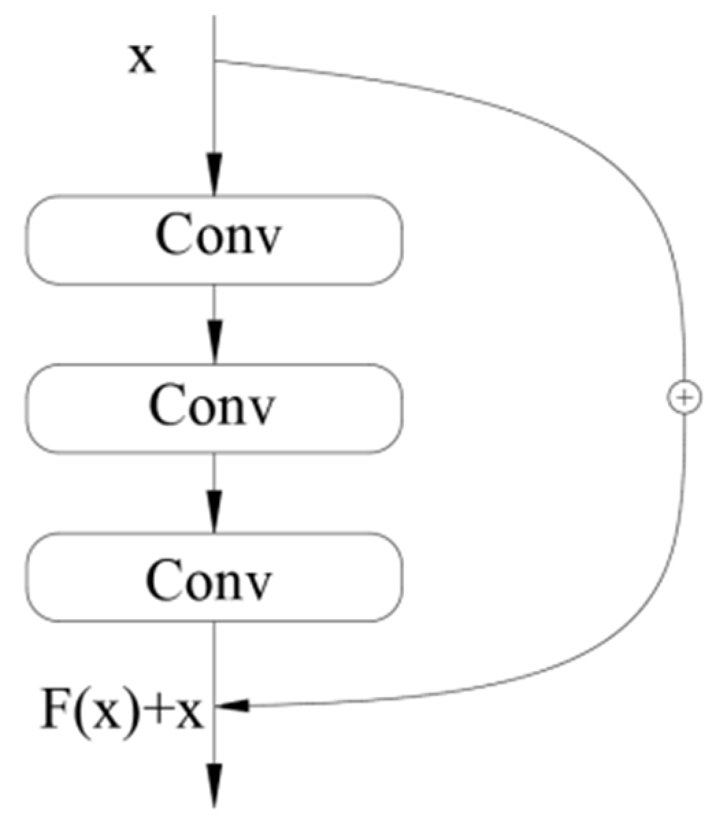
—the output of the residual block;
  • x l —input feature vector for the lth layer;
  • F ( x i , W i ) —the mapping function that needs to be learned;
  • W i —the projection matrix.
The basic model is established according to the ResNet structure. After pretraining on ImageNet, the convolutional layer is used as the feature extraction structure, and the bottom layer of the residual model is added to a fully connected layer as a classifier. The dropout function is added to the fully connected layer, as shown in Equation (5). The established residual model is trained, and the initial learning rate is 0.01. The loss function is the same as Equation (7), and the learning rate decreases with the increase of training time.
In this paper, the TensorFlow machine learning development platform is used to train the transfer learning model based on the ResNet model, and the indicator diagram classification experiment is carried out. The experimental environment is the NVIDIA Tesla T4 computing platform. The model is tested while the training set is trained, and the output of the training set and test set are recorded as shown in Figure 13a,b, respectively, and the test results are shown in Figure 13c. The recognition accuracy of the test set is 95.3%, the output loss of the test set is 0.618, and the single training time of the model is 8.021 s.
In Figure 13a,b, the abscissa represents the number of training times, the ordinate represents the training accuracy and output error of the model, respectively, and the two curves represent the training set and test set data, respectively. The experimental results show that the transfer learning model based on the ResNet model can basically complete the indicator diagram classification task. As can be seen from Figure 13a, the accuracy of the model increases rapidly in the early stage of training. Compared with the classic deep learning model, the transfer learning model has a faster growth rate in the early stage of training; after about 40 times of training, the model accuracy enters a gentle growth range, and then the training set accuracy gradually stabilizes at 1.
It can be seen from Figure 13b that the data loss trend of the training set is opposite to the accuracy rate. In the early stage of training, both the training set and the test set have a high degree of data loss, but it quickly drops to a normal level, and then the data loss decreases steadily until the trend is flat, entering the lower data loss range. In the flat interval, the data loss of the test set fluctuates less, but it is always larger than the training set, indicating that there is a certain deviation between the model and the actual situation. In Figure 13c, it can be seen that most of the test data can be accurately identified, but the recognition rate of the case types with a small number of samples is low, which is consistent with the data loss.
The Xception model extracts the graphic features by dividing them into several channels, as shown in Figure 14, which not only ensures that the image features can be fully extracted, but also effectively reduces the amounts of parameters and computation [21].
The basic model is established according to the Xception model structure. After pretraining on ImageNet, the convolutional layer is reserved as the feature extraction structure, and the fully connected layer is added as a classifier at the bottom of the Xception model. The dropout function is added to the fully connected layer, as shown in Equation (5). To train the transfer learning model based on the Xception model, the initial learning rate is 0.01, the loss function is the same as Equation (7), and the learning rate decreases with the increase of training time.
In this paper, using TensorFlow as the machine learning development platform, the classification experiment of the transfer learning model based on the Xception model is carried out. The experimental environment was the NVIDIA Tesla K80 computing platform, and the training set and model were tested simultaneously. Figure 15a,b record the output of the training set and test set, and the test results are shown in Figure 15c. The recognition accuracy of the test set is 95.3%, the output loss of the test set is 0.245, and the single training time of the model is 7.048 s.
In Figure 15a,b, the abscissa represents the number of training times, the ordinate represents the training accuracy and output error of the model, respectively, and the two curves represent the training set and test set data, respectively. The experimental results show that the transfer learning model based on the Xception model can basically complete the indicator diagram classification task. The experimental model has been trained a total of 140 times. In Figure 15a, it can be seen that the accuracy rate curve increases rapidly at the beginning of the training, and the accuracy rate curve enters a flat interval after 80 times of training; in the growth interval, the test set curve and the training set curve partially intersect; the test set curve is slightly lower than the training set after entering the flat interval.
As can be seen in Figure 15b, the data loss in the initial stage of training is large but decreases rapidly, and then the overall level tends to be flat, and the model reaches a better state at this time. Compared with the test results in Figure 15c, although the accuracy of the test set is generally good, the recognition rate of the model is not high for a single working condition. From the data in the figure, it can be seen that a small number of working condition types have better accuracy.
The basic unit of the MobileNet model is separable convolution (DW Conv). Compared with traditional convolution operations, it can be divided into two parts: firstly, the corresponding convolution kernels are applied in different channels to extract information, and then 1 × 1 convolution kernels are applied in each classification channel to change the shape of feature maps. The process is shown in Figure 16 [22].
The basic model is established according to the above structure, and after pretraining on ImageNet, the convolutional layer is reserved as the feature extraction structure. A typical MobileNet model does not contain a fully connected layer at the bottom. In this paper, a fully connected layer is added as a classifier at the bottom of the feature extraction layer, and a dropout layer is added to the fully connected layer. The transfer learning model based on the MobileNet model is trained and the initial learning rate is 0.01. The loss function is the same as above. The learning rate decreases with the increase of training time.
This paper uses the TensorFlow machine learning development platform to conduct the dynamometer classification experiment of the transfer learning model based on the MobileNet model. The experimental environment is the NVIDIA Tesla K80 computing platform. The model is tested while the training set is being trained, and the output of the training set and test set are recorded as shown in Figure 17a,b, and the test results are shown in Figure 17c. The recognition accuracy of the test set is 97.3%, the output loss of the test set is 0.211, and the single training time of the model is 5.003 s.
In Figure 17a,b, the abscissa represents the number of training times, the ordinate represents the training accuracy and output error of the model, respectively, and the two curves represent the training set and test set data, respectively. The experimental results show that the transfer learning model based on the MobileNet model can complete the indicator diagram classification task. The experimental model is trained a total of 100 times. In Figure 17a, it can be seen that the accuracy curve increases rapidly in the early stage of training. After 40 times of training, the curve enters a flat range, and the training set curve converges to around 99%; in the growth range, the test set curve has is a partial intersection with the training set curve, so it can be seen that there is no overfitting phenomenon.
As can be seen in Figure 17b, the overall trend of the loss curve and the accuracy rate curve basically correspond one-to-one; the loss rate curve shows a logarithmic trend of decline, and enters a flat range after 60 training sessions. The curve of the test set is stable in the flat range, and the overall curve is slightly higher than that of the training set, which proves that the MobileNet model deviates from reality. Comparing the test results in Figure 17c, it can be seen from the data in the figure that the accuracy of a small number of working condition types is better, and the recognition rate of the model for a single working condition type is not high. The performance of the model on the test atlas shows that the transfer learning model based on the MobileNet model can accurately identify the characteristics of some types of working conditions but cannot identify all characteristics of the 15 types of working conditions.
Table 3 shows the comparison results of the ResNet, MobileNet, Xception, and DenseNet models. Each comparison model performs very well in the training set and test set, but due to the serious uneven distribution of the number of samples, the recognition rate of a single type of indicator diagram varies greatly. From the analysis of the training curve, the initial loss value of the Xception model is high, but the convergence speed is fast and the curve is stable. At the same time, it can better identify the fault types with sufficient samples, which can be applied in the case of a small number of classifications.
The loss data of the test set of the ResNet model still fluctuates significantly when the training set enters the stable range, and the accuracy of the test set is significantly lower than that of the training set, which proves that there is a certain degree of overfitting. The final training result of the MobileNet model is only 42.8 MB, which is the smallest of all the models, and the overall accuracy of the model is good, but the recognition rate for some working conditions is poor
The recognition rate of the DenseNet model is generally at a good level. Except for the influence of heavy oil, the recognition rate of various working conditions is higher than 90%; in a single type of fault type, the recognition rate is lower than that of the fault type, such as the broken rod. The off-time is lower than ResNet and Xception, but its average recognition rate far exceeds that of the control group classification model, proving that it can effectively classify 15 types of working conditions

4. Conclusions

Based on the structure of DenseNet model, this paper uses the global pooling layer to replace the full connection classification layer in the classical model, and classifies 15 kinds of working conditions, such as plunger bump, plunger down bump, insufficient fluid supply, double vale loss, fixed vale loss, and broken rod. Using the pretraining model 698 and training of ImageNet, transfer learning is carried out on the production data set of Daqing Oilfield, and then different structural models are trained under the same conditions. The results are compared, and the following conclusions are obtained:
  • The DenseNet model is an image classification model with the characteristics of parameter reuse, which can effectively use limited training images to obtain feature information. In this paper, based on the DenseNet model, an indicator diagram classification model is established employing transfer learning, good classification results are obtained, and the accuracy rate of the test set can reach 96.9%.
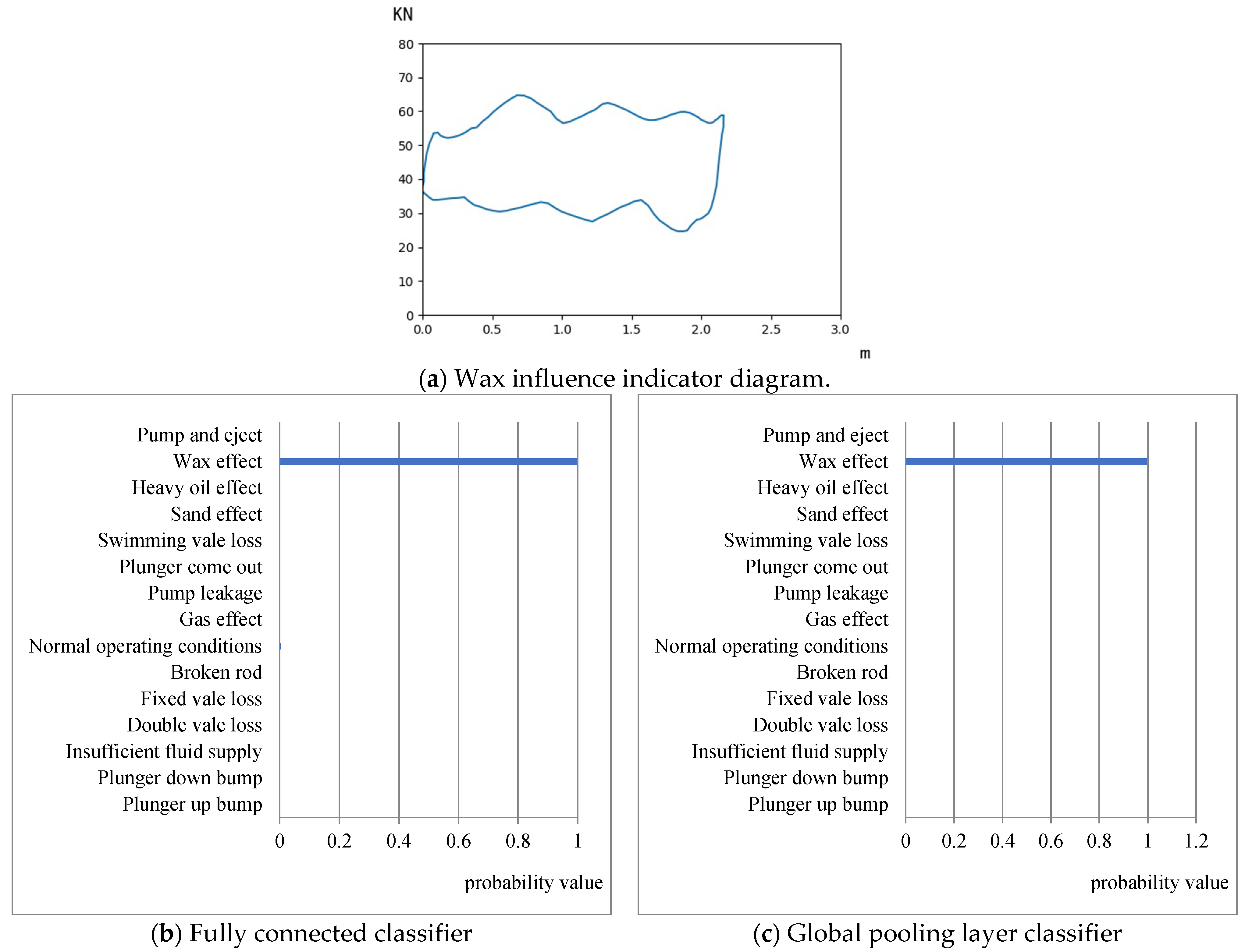
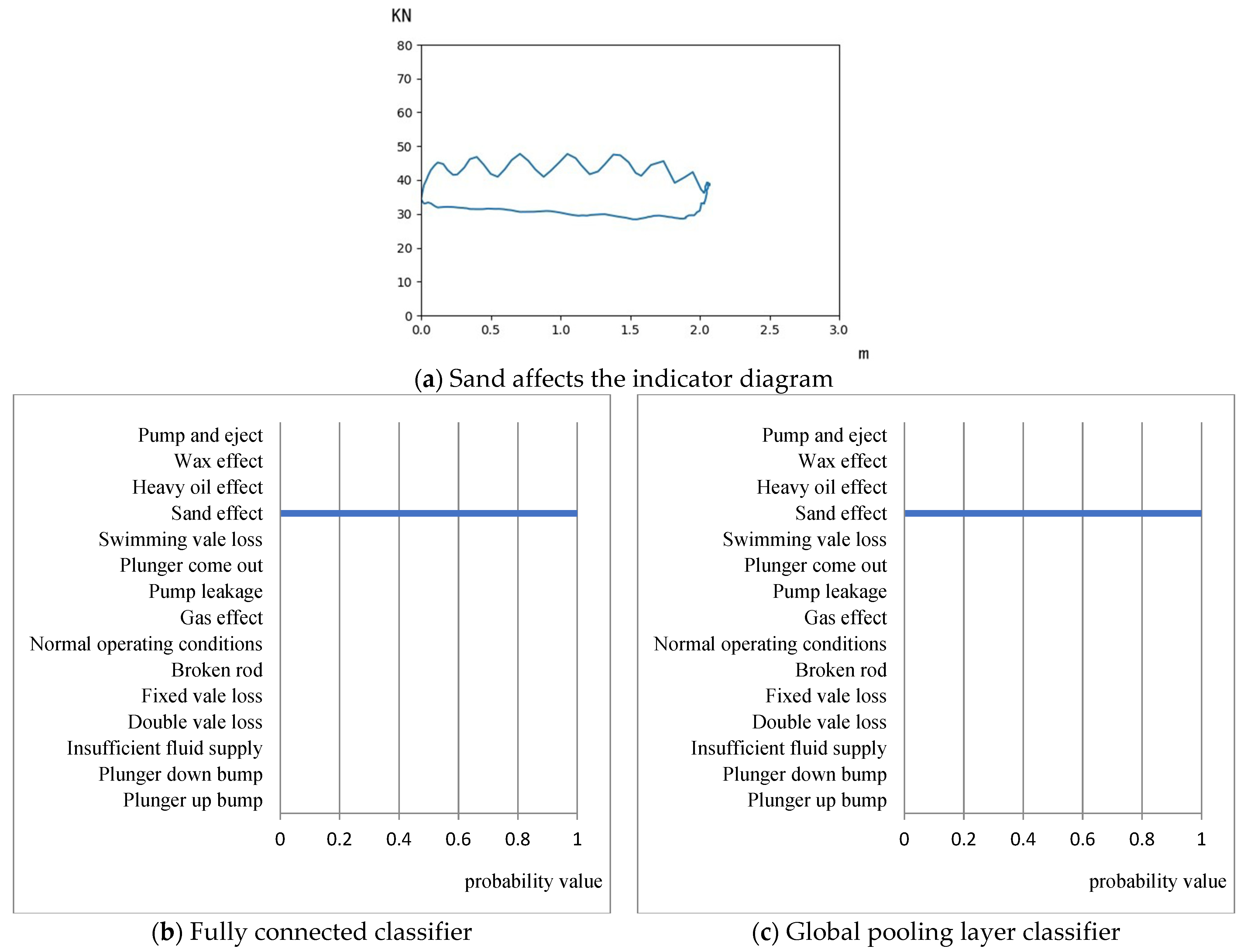
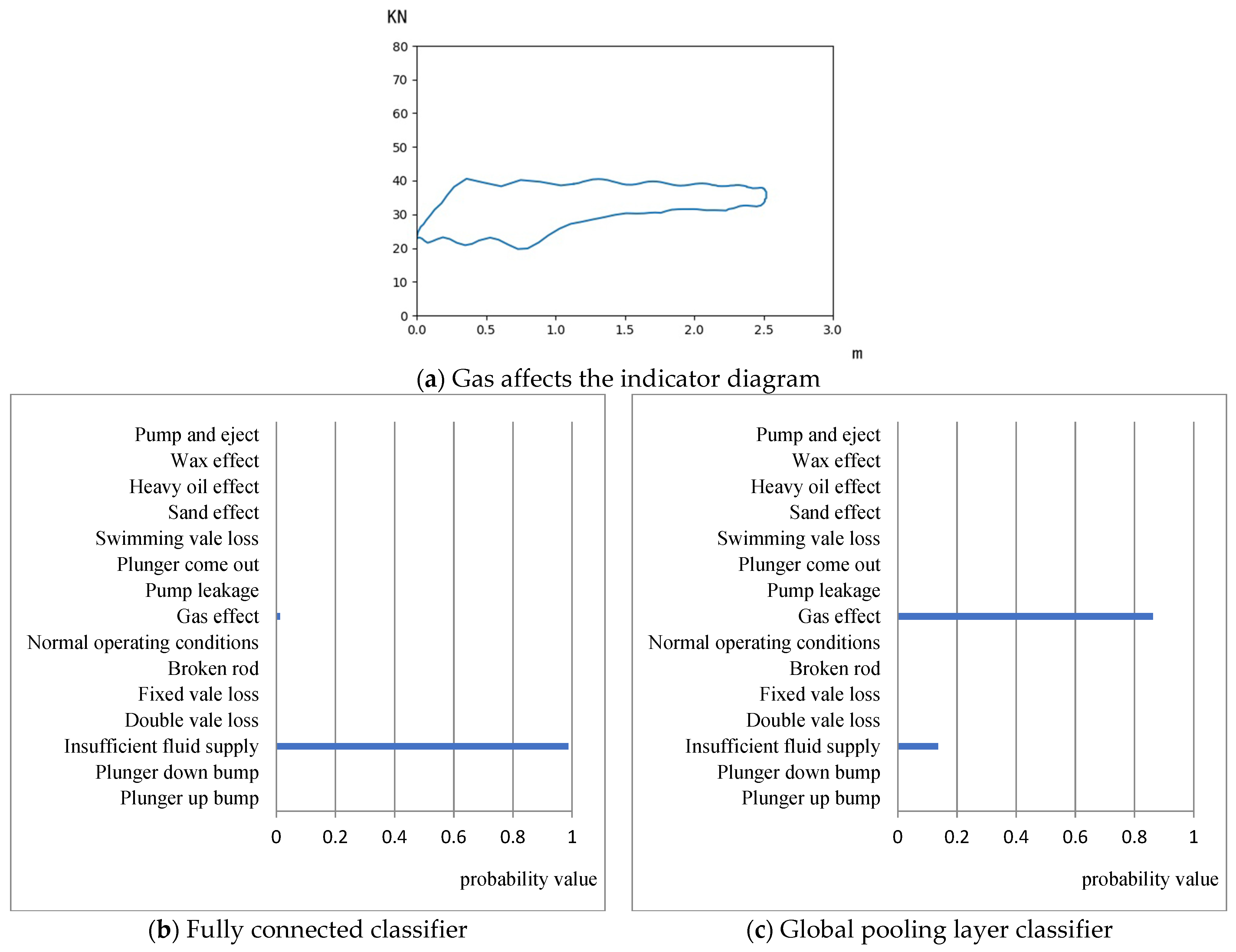
  • The full connection classifier and the global pooling classifier are used to build the classification model, respectively. The results of the two types of models under the same training mechanism and using the same data set for transfer learning show that the classification effect of the global pooling classification model is better than that of the full connection. The layer classification model can be well adapted to the classification task of the indicator diagram, and the recognition rate of various working conditions generally reaches more than 90%. Among them, the recognition rate of double valve loss and pump and eject reached 100%, the lowest recognition rate was 87%, under the influence of heavy oil, and the average recognition rate of 15 types of operating conditions was 95.8%, far exceeding the control group
  • The training results of the transfer learning classification model based on DenseNet show that the parameter reuse structure and transfer learning method can improve the overfitting problem of small data sets in machine learning models. The difference between the average accuracy of the training set and the test set of the DenseNet transfer learning classification model in the flat interval is only 2.7%, which can avoid the problem of a small number of samples falling in classification due to uneven data. The recognition rates of the ResNet, MobileNet, and Xception models for plunger-up bump conditions are all below 30%. The MobileNet model has a recognition rate of only 4.3% for plunger bump, while the DenseNet-based transfer learning classification model has a recognition rate of 91.3% for plunger bump.
  • The comparison of the recognition model shows that the overall accuracy rate of the data set is basically the same as that of the DenseNet-based transfer learning model compared with ResNet, MobileNet, and Xception. However, compared with the control group model, the accuracy of a single type, such as plunger up bump, plunger down bump, and heavy oil effect, has been significantly improved, and the number of classifications can be further explored.
  • The fault diagnosis model of the pumping unit based on the DenseNet model and transfer learning can solve the problem that the automatic fault technology based on the machine learning algorithm cannot recognize all kinds of working conditions due to insufficient production data and uneven quantity of all kinds of data. The model expands the number of identifiable working conditions and can better adapt to the actual working conditions, further supplementing the theory and technology of fault diagnosis for pumping wells.

Author Contributions

Z.F.: Advisor, Conceptualization, Methodology, Writing—Review and Editing. Y.W.: Conceptualization, Methodology. Q.L.: Numerical Simulation, Data curation, and Visualization. J.L.: Conceptualization, Data Curation and Visualization. D.S.: Writing—Review and Editing. All authors have read and agreed to the published version of the manuscript.

Funding

The project was funded by the Natural Science Foundation of China (No.51774091), Heilongjiang Postdoctoral Scientific Research Developmental Fund (No.LBH-Q20083).

Institutional Review Board Statement

Not applicable.

Informed Consent Statement

Not applicable.

Data Availability Statement

Not applicable.

Acknowledgments

Thanks to my graduate students for their help.

Conflicts of Interest

The authors declare that there are no other conflicts of interest.

References

  1. Derek, H.J.; Jennings, J.W.; Morgan, S.M. Sucker Rod Pumping Unit Diagnostics Using an Expert System. In Proceedings of the Permian Basin Oil and Gas Recovery Conference, Midland, TX, USA, 10–11 March 1988. [Google Scholar] [CrossRef]
  2. Rogers, J.D.; Guffey, C.G.; Oldham, W.J.B. Artificial Neural Networks for Identification of Beam Pump Dynamometer Load Cards. In Proceedings of the SPE Annual Technical Conference and Exhibition, New Orleans, LA, USA, 23–26 September 1990. [Google Scholar] [CrossRef]
  3. Nazi, G.M. Application of Neural Artificial Network to Pump Card Diagnosis. SPE Comput. Appl. 1994, 10, 9–14. [Google Scholar] [CrossRef]
  4. Wen, B.L.; Wang, Z.Q.; Jin, Z.Z.; Xu, M.; Shi, Z. Diagnosis of Pumping Unit with Combing Indicator Diagram with Fuzzy Neural Networks. Comput. Syst. Appl. 2016, 25, 121–125. [Google Scholar]
  5. Rauber, T.W.; Boldt, F.A.; Varejão, F.M. Heterogeneous feature models and feature selection applied to bearing fault diagnosis. IEEE Trans. Ind. Electron. 2014, 62, 637–646. [Google Scholar] [CrossRef]
  6. Chine, W.; Mellit, A.; Lughi, V.; Malek, A.; Sulligoi, G.; Massi Pavan, A. A novel fault diagnosis technique for photovoltaic systems based on artificial neural networks. Renew. Energy 2016, 90, 501–512. [Google Scholar] [CrossRef]
  7. Dumidu, W.; Ondrej, L.; Milos, M.; Craig, R. FN-DFE: Fuzzy-neural data fusion engine for enhanced resilient state-awareness of hybrid energy systems. IEEE Trans. Cybern. 2014, 44, 2065–2075. [Google Scholar] [CrossRef]
  8. Chen, H.P.; Hu, N.Q.; Cheng, Z.; Zhang, L.; Zhang, Y. A deep convolutional neural network based fusion method of two-direction vibration signal data for health state identification of planetary gearboxes. Measurement 2019, 146, 268–278. [Google Scholar] [CrossRef]
  9. Olivier, J.; Viktor, S.; Bram, V.; Kurt, S.; Mia, L.; Steven, V.; Rik, V.W.; Sofie, V.H. Convolutional neural network based fault detection for rotating machinery. J. Sound Vib. 2016, 377, 331–345. [Google Scholar] [CrossRef]
  10. Zhao, H.; Wang, J.; Gao, P. A deep learning approach for condition-based monitoring and fault diagnosis of rod pump system. Serv. Trans. Internet Things 2017, 1, 32–42. [Google Scholar] [CrossRef]
  11. Wang, X.; He, Y.F.; Li, F.J.; Dou, X.J.; Wang, Z.; Xu, H.; Fu, L.P. A Working Condition Diagnosis Model of Sucker Rod Pumping Wells Based on Big Data Deep Learning. In Proceedings of the International Petroleum Technology Conference, Beijing, China, 26–28 March 2019; pp. 1–10. [Google Scholar] [CrossRef]
  12. Cheng, H.; Yu, H.; Zeng, P.; Osipov, E.; Li, S.; Vyatkin, V. Automatic Recognition of Sucker-Rod Pumping System Working Conditions Using Dynamometer Cards with Transfer Learning and SVM. Sensors 2020, 20, 5659. [Google Scholar] [CrossRef] [PubMed]
  13. Mao, W.T.; He, L.; Yan, Y.J.; Wang, J.W. Online sequential prediction of bearings imbalanced fault diagnosis by extreme learning machine. Mech. Syst. Signal Process. 2017, 83, 450–473. [Google Scholar] [CrossRef]
  14. Bengio, G.L.; Courville, Y. A Deep Learning; MIT Press: Cambridge, MA, USA, 2016; Volume 1, pp. 326–366. [Google Scholar]
  15. Lecun, Y.; Bottou, L.; Bengio, Y.; Haffner, P. Gradient-based learning applied to document recognition. Proc. IEEE 1998, 86, 2278–2324. [Google Scholar] [CrossRef] [Green Version]
  16. Yu, D.J.; Wang, H.L.; Chen, P.Q.; Wei, Z.H. Mixed pooling for convolutional neural networks. In Proceedings of the International Conference on Rough Sets and Knowledge Technology, Shanghai, China, 24–26 October 2014; Springer: Cham, Switzerland, 2014; pp. 364–375. [Google Scholar] [CrossRef]
  17. Huang, G.; Liu, Z.; Maaten, L.; Kilian, Q.; Weinberger, K.Q. Densely connected convolutional networks. In Proceedings of the IEEE Conference on Computer Vision and Pattern Recognition, Honolulu, HI, USA, 21–26 July 2017; pp. 4700–4708. [Google Scholar] [CrossRef] [Green Version]
  18. Kingma, D.; Adam, B.J. A Method for Stochastic Optimization. In Proceedings of the 3rd International Conference for Learning Representations, San Diego, CA, USA, 7–9 May 2015. [Google Scholar] [CrossRef]
  19. Yosinski, J.; Clune, J.; Bengio, Y.; Lipson, H. How transferable are features in deep neural networks? Adv. Neural Inf. Process. Syst. 2014, 27, 3320–3328. [Google Scholar]
  20. He, K.; Zhang, X.; Ren, S.; Sun, J. Deep Residual Learning for Image Recognition. In Proceedings of the 2016 IEEE Conference on Computer Vision and Pattern Recognition (CVPR), Las Vegas, NV, USA, 27–30 June 2016; pp. 770–778. [Google Scholar] [CrossRef] [Green Version]
  21. Chollet, F. Xception: Deep Learning with Depthwise Separable Convolutions. In Proceedings of the 2017 IEEE Conference on Computer Vision and Pattern Recognition (CVPR), Honolulu, HI, USA, 21–26 July 2017; pp. 1800–1807. [Google Scholar] [CrossRef] [Green Version]
  22. Howard, A.G.; Zhu, M.; Chen, B.; Kalenichenko, D.; Wang, W.; Weyand, T.; Andreetto, M.; Adam, H. MobileNets: Efficient Convolutional Neural Networks for Mobile Vision Applications. arXiv 2017, arXiv:1704.04861. [Google Scholar] [CrossRef]
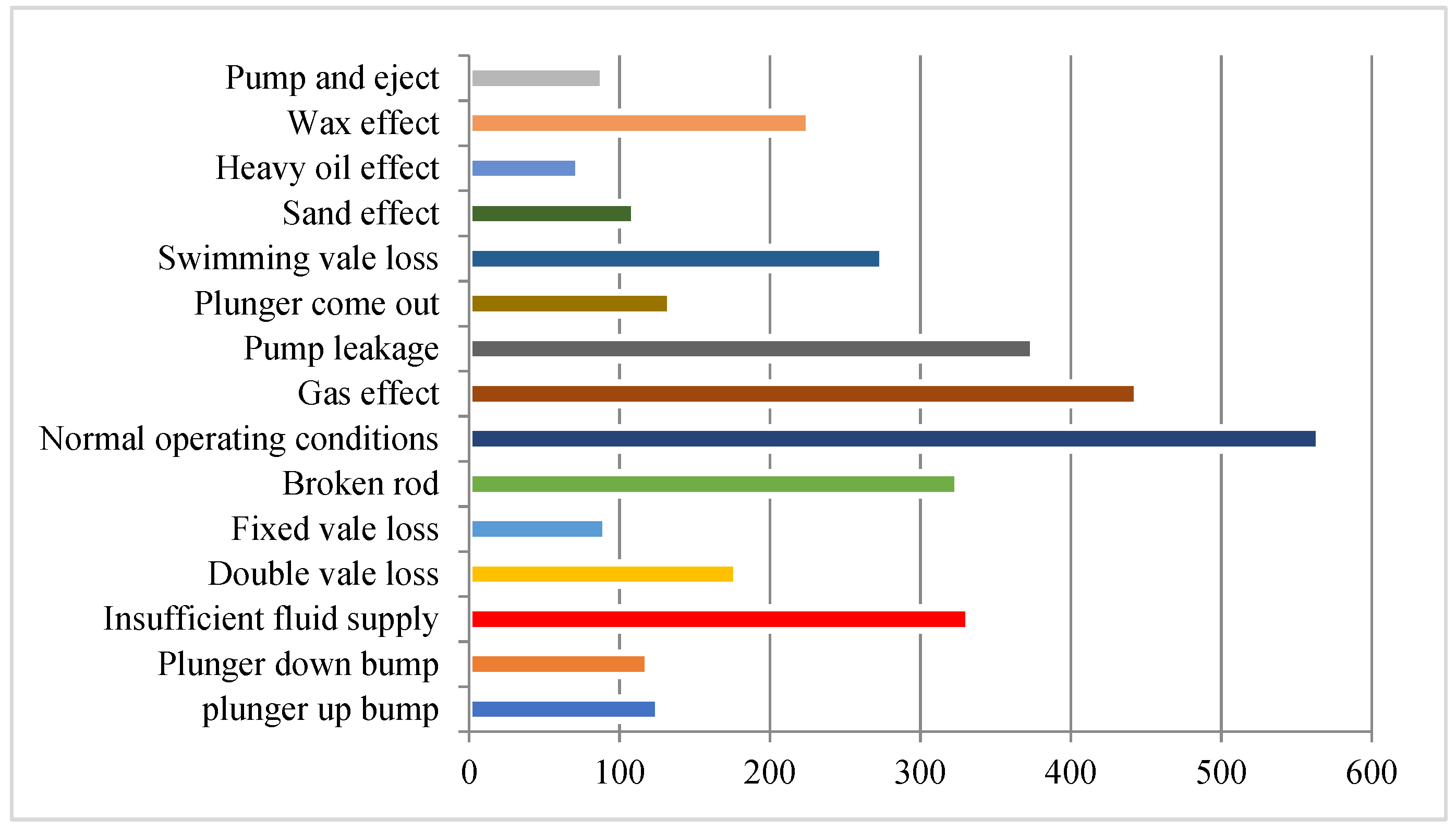
Figure 1. Distribution diagram of actual working condition data.
Applsci 12 11091 g001
Figure 2. Theoretical indicator diagram under static load.
Applsci 12 11091 g002
Figure 3. Example of Dynamometer Fault Types.
Applsci 12 11091 g003
Figure 4. Diagram of convolutional neural network image recognition process.
Applsci 12 11091 g004
Figure 5. Dense connection mode of DenseNet model.
Applsci 12 11091 g005
Figure 6. Densely connected model applying global pooling layer classifier.
Applsci 12 11091 g006
Figure 7. Model training results of the fully connected layer classifier of the densely connected model.
Applsci 12 11091 g007
Figure 8. Test results of working conditions affected by wax.
Applsci 12 11091 g008
Figure 9. Sand affects the test results of working conditions.
Applsci 12 11091 g009
Figure 10. Gas affects the test results of working conditions.
Applsci 12 11091 g010
Figure 11. Test results under normal conditions.
Applsci 12 11091 g011
Figure 12. ResNet structure.
Applsci 12 11091 g012
Figure 13. Transfer learning model training results based on ResNet model.
Applsci 12 11091 g013
Figure 14. Basic structure of the Xception model.
Applsci 12 11091 g014
Figure 15. Training results of the transfer learning model based on the Xception model.
Applsci 12 11091 g015
Figure 16. MobileNet model.
Applsci 12 11091 g016
Figure 17. Training results of the transfer learning model based on the MobileNet model.
Applsci 12 11091 g017
Table 1. Label index assignment result.
Fault TypeIndexNumber
Plunger up bump0126
Plunger down bump1119
Insufficient fluid supply2332
Double valve loss3178
Fixed valve loss491
Broken rod5325
Normal operating conditions6565
Gas effect7444
Pump leakage8375
Plunger come out9134
Swimming valve loss10275
Sand effect11110
Heavy oil effect1273
Wax effect13226
Pump and eject1489
Table 2. Single fault type and overall recognition rate.
Fault TypeRecognition Rate
Fully Connected LayerGlobal Pooling Layer
plunger up bump66.0%91.3%
plunger down bump59.1%90.9%
insufficient fluid supply94.9%97.5%
double valve loss62.9%100.0%
fixed valve loss81.8%90.9%
broken rod95.5%97.7%
normal operating conditions94.9%100.0%
gas effect93.5%97.8%
pump leakage100.0%99.1%
plunger come out90.5%100.0%
swimming valve loss76.7%98.6%
sand effect71.4%90.5%
heavy oil effect87.5%87.5%
wax effect80.9%95.6%
pump and eject50.0%100.0%
training set accuracy99.6%100.0%
test set accuracy96.9%96.9%
Table 3. Comparison of recognition rate of various models.
Fault TypeRecognition Rate
ResNetMobileNetXceptionDenseNet
plunger up bump8.6%4.3%21.7%91.3%
plunger down bump22.7%54.5%45.5%90.9%
insufficient fluid supply86.6%75.9%67.1%97.5%
double vale loss89.1%48.6%48.6%100.0%
fixed vale loss0%18.2%45.5%90.9%
broken rod95.4%77.3%100.0%97.7%
normal operating conditions100%46.2%84.6%100.0%
gas effect97.8%41.3%91.3%97.8%
pump leakage86.9%94.3%47.2%99.1%
plunger come out0%28.6%23.8%100.0%
swimming vale loss80.8%47.9%54.8%98.6%
sand effect19%95.2%71.4%90.5%
heavy oil effect0%12.5%62.5%87.5%
wax effect91.1%97.1%58.8%95.6%
pump and eject0%16.7%66.7%100.0%
Training set100.0%99.3%98.6%99.8%
Testing set95.3%97.4%95.3%96.9%
Average recognition rate51.8%50.5%59.3%95.8%
Publisher’s Note: MDPI stays neutral with regard to jurisdictional claims in published maps and institutional affiliations.

