Model Predictive Control of Running Biped Robot

Abstract

With the feet of a biped robot attached insecurely to a terrain, its stability is strongly affected by the characteristics of the terrain on which it runs. Therefore, for stable bipedal running, online motion control based on the states of the robot and the environment is needed. This paper proposes a method for online motion control of a running biped robot on an uneven terrain based on a dual linear inverted pendulum model (D-LIPM) and hierarchical control which consists of linear model predictive control (MPC) and quadratic-problem (QP) based momentum control. The D-LIPM, which splits the nonlinear dynamics model of the running biped robot into two linear models under some assumptions, is proposed to generate the running motion through linear MPC. The D-LIPM is applied to the proposed hierarchical control for stable bipedal running. In the first stage of hierarchy, linear MPC is employed to generate the trajectory of the center of mass (COM) based on the dynamics of D-LIPM to overcome terrain uncertainties such as elevation levels and surface conditions at foot-landing sites. In the second stage, momentum control based on a QP solver is used to generate the angular motions of the robot while following the COM trajectory. Computer simulations with uncertainties on the running terrain were carried out to measure the performance of the proposed method.

1. Introduction

Legged robots should be able to adapt to a variety of environments including ones with unstructured and discontinuous ground [1,2,3,4]. Among the legged robot, a moving biped robot can easily become unstable because its dynamics are highly nonlinear than other legged robots, and the application of the robot is limited in the real world, despite their potential capability. Until now, so many studies have been carried out to overcome this limitation [5,6,7,8,9,10,11].

Running is a dynamic and challenging locomotion method of a biped robot. Raibert et al. were the first to research running biped robots; they successfully used a spring-loaded inverted pendulum (SLIP) model for a hopping robot [12,13]. Several studies have used the SLIP model to generate a running trajectory for a biped robot [14,15,16]. As an alternative, a few studies have used an inverted pendulum model (IPM) for running biped robots. Kajita proposed a feedback controller based on a linear inverted pendulum model (LIPM) for running [17,18]. Tajima proposed a motion planning method based on the height of the center of mass (COM) and angular momentum of a biped robot [19]. These methods generate a trajectory for a predefined environment. However, it is impossible to obtain all relevant information about the environment in advance, thus methods to generate robot motion online are needed [20].

For the stable running of a biped robot against disturbances and uncertainties in the environment, studies on online running motion generation based on its dynamic states have been carried out. Geyer and Nir proposed motion generation methods based on swing leg retraction (SLR) for a bipedal running on uneven terrain [21,22]. However, the SLR required a process to generate a predefined map of the angles at apex heights. As another approach, quadratic program (QP) based methods were proposed in [23,24]. These QP-based methods only considered instantaneous situations [25], and thus the information about the future states of the robot cannot be considered, resulting that recursive feasibility cannot be guaranteed. To address the issue of QP-based methods, a trajectory optimization-based method was proposed in [26], which has the drawback of a long computational time. An online re-planning method can be used as a solution to the problem, and model predictive control (MPC), which is one of the re-planning methods, has gained broad interest [27].

MPC is one of the control methods used to generate online motion. Its most important feature is its ability to handle constraints on the states and inputs of a dynamic system to select an optimized behaviour using model-based prediction [28]. As a result, MPC would have a robust and flexible behavior against unmodelled dynamics based on the predictive horizon with its states [29,30]. For the stable locomotion of a biped robot, a stable trajectory generation under the constraints on its workspace with robustness is critical. Therefore, several studies used MPC for bipedal locomotion. Wieber et al. generated a trajectory for walking of a humanoid robot based on the MPC with zero moment point (ZMP) preview control and showed in simulations that stable walking was achieved despite some disturbances [31]. Scianca proposed an intrinsically stable MPC framework for humanoid gait generation that incorporated a stability constraint based on the velocity of ZMP in the formulation and realized omnidirectional motion in real time [32]. Many MPC-based studies have focused on bipedal walking, but there is limited work on bipedal running.

Because the dynamics of a running biped robot are nonlinear, it is difficult to generate running motion with linear MPC. A method to control a nonlinear motion such as hopping with a nonlinear MPC was proposed in [33]. However, the nonlinear MPC suffers from drawbacks of a non-convex optimization problem such as long computational time and local minimum [34]. As one of the methods for generating a nonlinear motion including a time-varying vertical trajectory, MPC with a divergent component of motion (DCM) has been proposed under the assumption of a predefined vertical trajectory, thus making it difficult to generate a real-time running trajectory [35,36].

To address the problem of MPC with a nonlinear dynamics model and to generate a stable online running motion of a biped robot, this paper proposes a method to control a running biped robot based on a dual linear inverted pendulum model (D-LIPM) and hierarchical control with linear MPC and momentum control. D-LIPM, which splits the nonlinear dynamics model of the running biped robot into two linear models under some assumptions, is proposed to generate the running motion through linear MPC. The D-LIPM is applied to the proposed hierarchical control for stable bipedal running. In the first stage of hierarchy, linear MPC with a constraint for stability using a friction cone is employed to generate the COM trajectory based on D-LIPM to overcome terrain uncertainties such as elevation levels and surface conditions at foot-landing sites. In the second stage, momentum control based on a QP solver with constraints on the workspace is applied to follow the COM trajectory. For performance validation of the proposed method, computer simulations of running with uncertainties on the terrain were conducted. The key contributions made by this paper are:

(1)

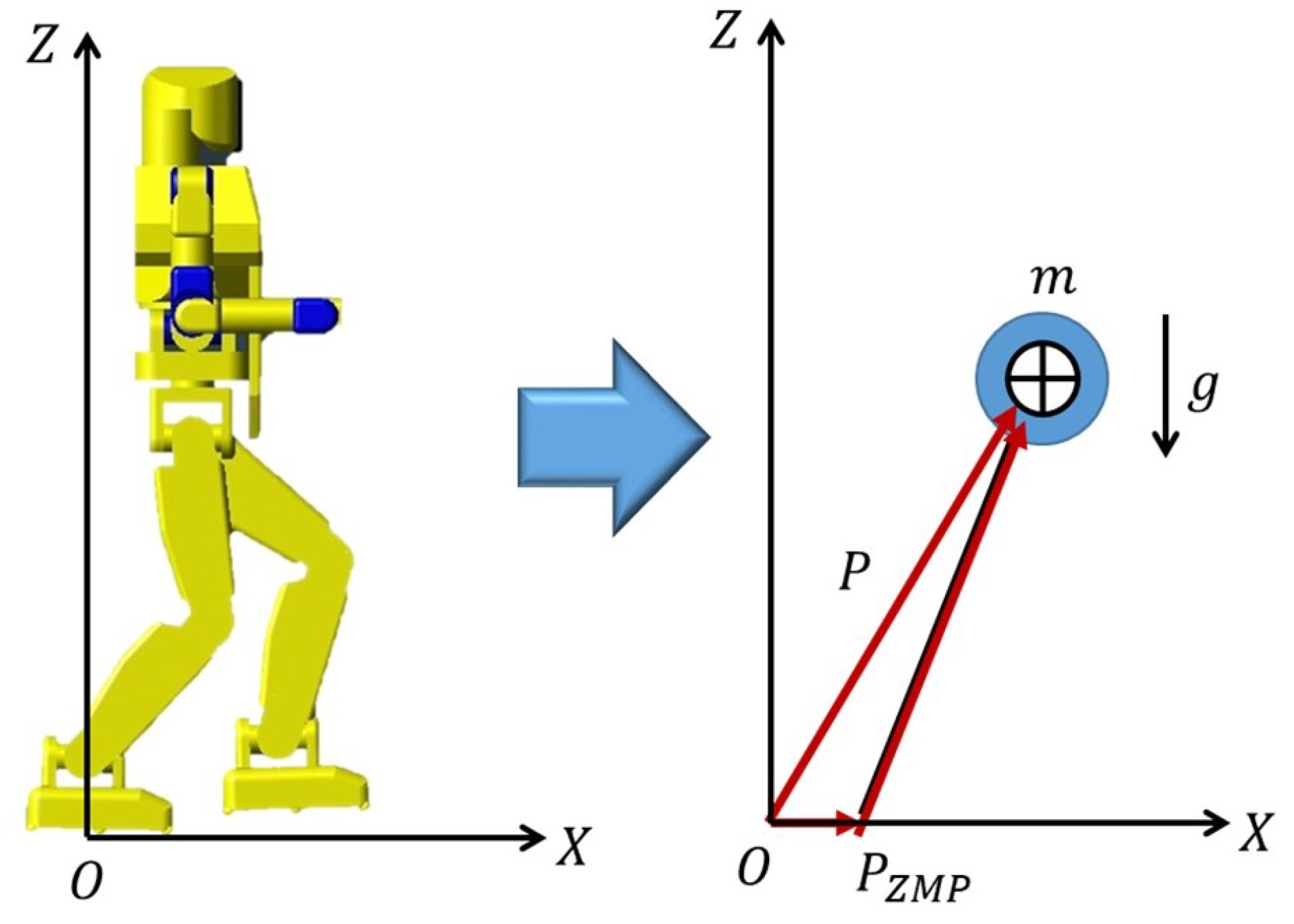
D-LIPM is proposed to be used instead of a nonlinear dynamic model of a biped robot.

(2)

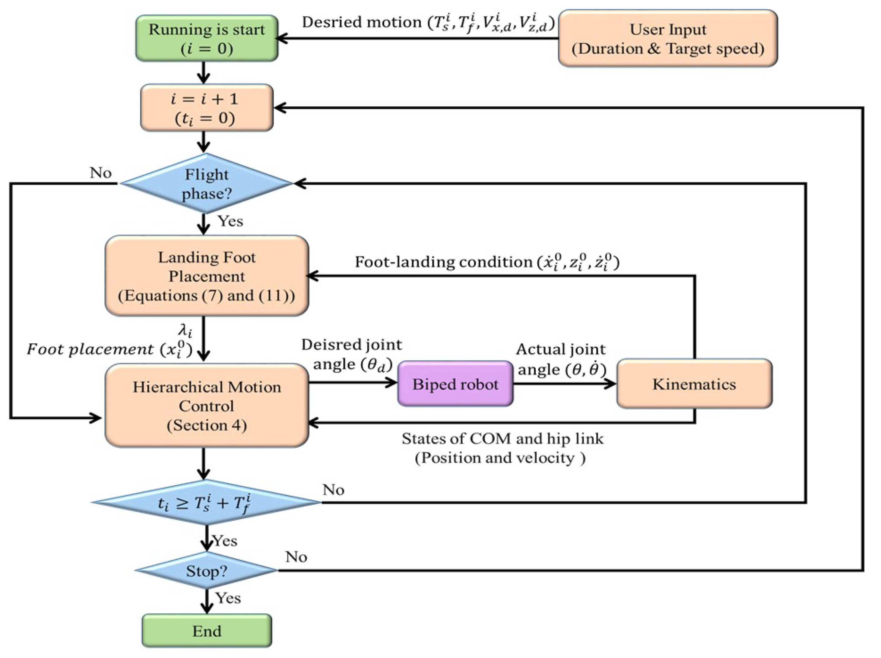
To overcome terrain uncertainties and generate the online running motion of a biped robot, hierarchical motion control with linear MPC and QP-based momentum control is proposed.

(3)

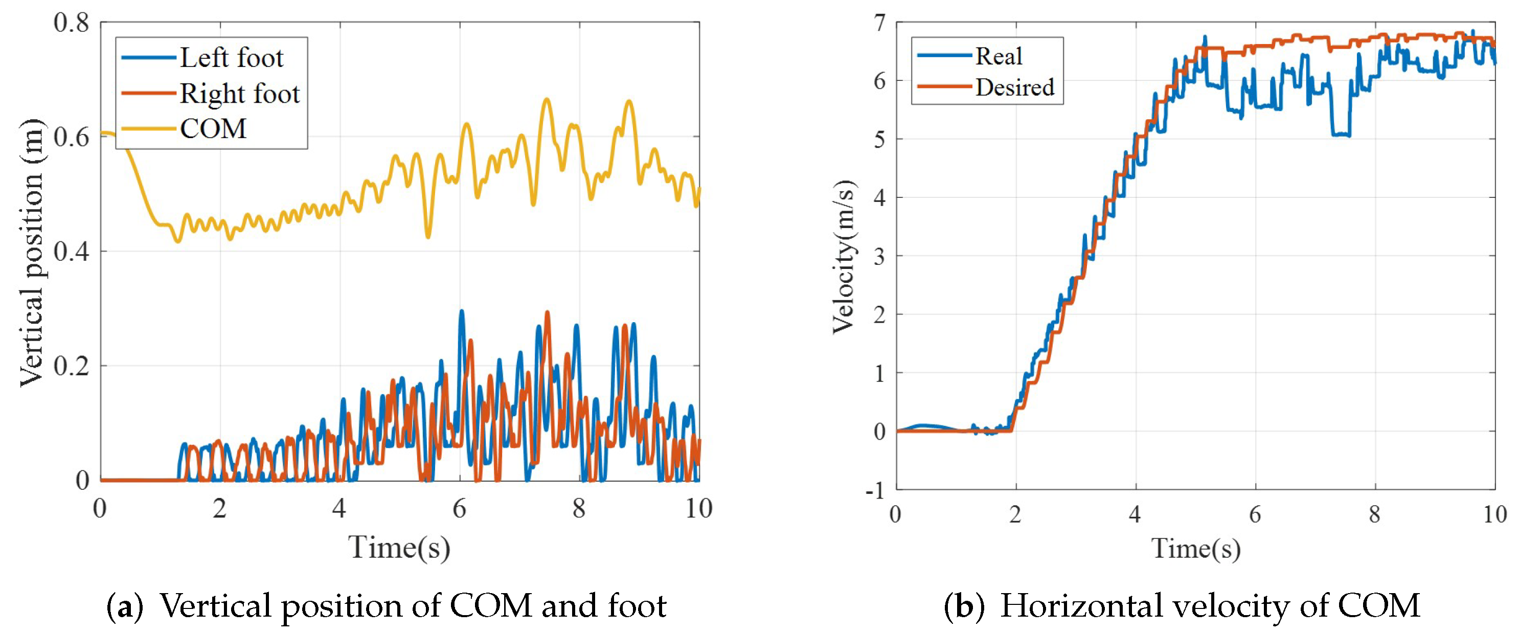
Simulations showed that a biped robot could run at 6.5 m/s even with unobserved obstacles whose height was approximately 10 % of the length of its legs.

The remainder of this paper is organized as follows. A centroidal dynamics model for a running biped robot is described in Section 2. A method to find foot placement for running is discussed in Section 3. In Section 4, the proposed hierarchical online control for the running of the robot is explained. In Section 5, the performance of the proposed method is measured, and its effectiveness is shown through simulations, followed by a few conclusions in Section 6.

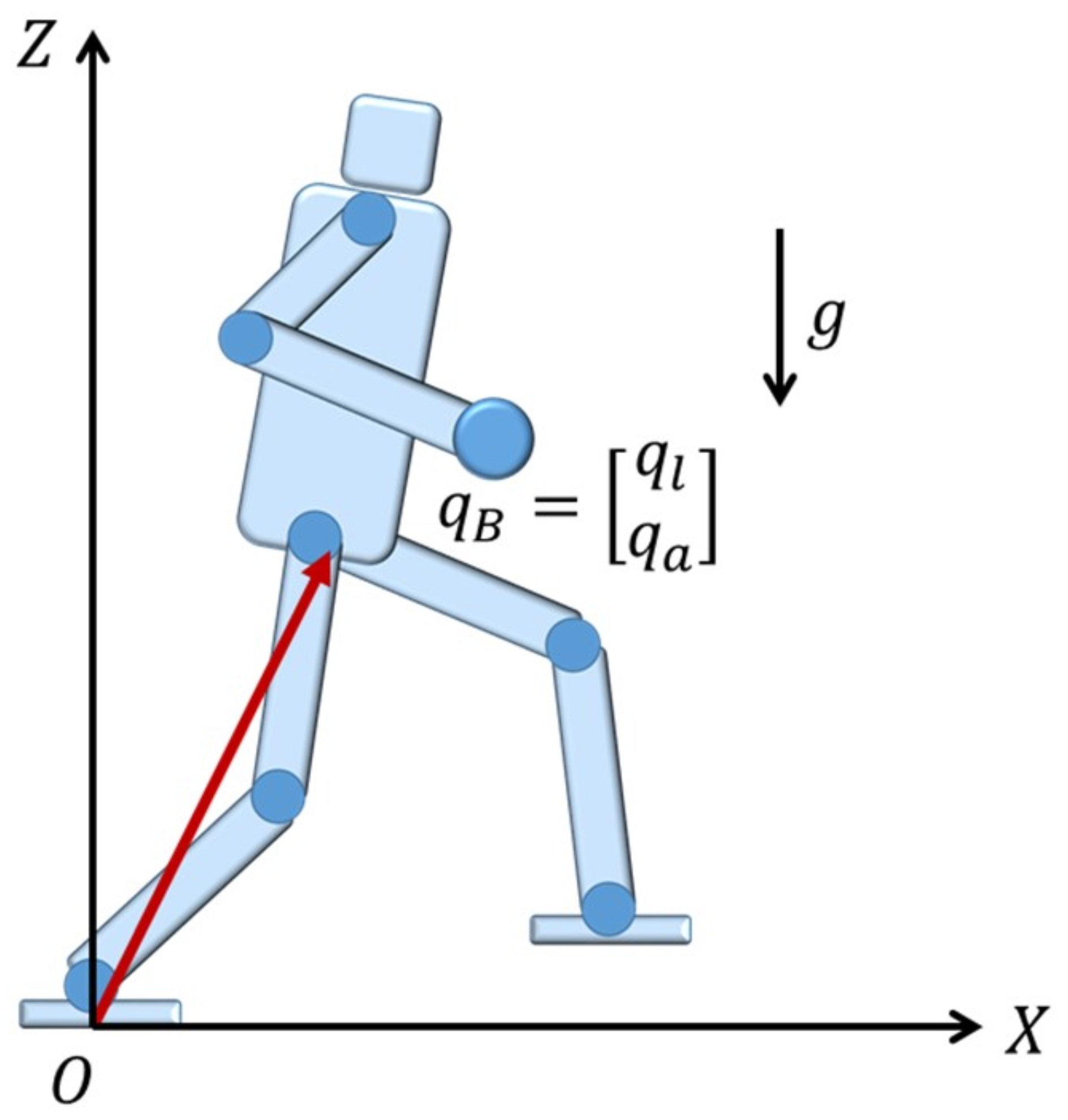
2. Model of Biped Robot

Since the dynamics of a biped robot is nonlinear, it is difficult to generate a running trajectory of a biped robot by using a linear MPC. To address this problem, the model of a biped robot is designed as D-LIPM, which is split into two sub-models: horizontal and vertical models.

For the D-LIPM, the biped robot is assumed as a single mass with a ground contact through a mass-less bar, an IPM, as shown in Figure 1, a single mass of m, located at the COM of the robot, represents the whole body of the robot; point O which is the origin of the X-Y Cartesian coordinate frame denotes the center of the foot on the ground in a support phase; $P={\left[xyz\right]}^T$ denotes the position of the COM of the biped robot; and $P_{ZMP}={\left[x_{ZMP}{y}_{ZMP}0\right]}^T$ denotes the ZMP at which the resultant ground reaction force (GRF) is applied.

The dynamics of this simplified model [18] in the sagittal plane during support phase i can be written as

$$\begin{array}{ccc}\hfill {\ddot{x}}_i\left(t_i\right)& =& \frac{g+{\ddot{z}}_i\left(t_i\right)}{z_i\left(t_i\right)}\left(x_i\left(t_i\right)-x_i^{ZMP}\right),(0\le t_i\le T_s^i),\hfill \end{array}$$

(1)

where $t_i$ denotes the time during i-th phase, since the landing foot landed on the ground at the end of flight phase $i-1$. $T_s^i$ denotes the duration of the support phase i; $x_i$ and $z_i$ denote the horizontal and vertical position of the COM, respectively; g denotes the gravitational acceleration, and $x_i^{ZMP}$ denotes the horizontal coordinate of the ZMP. To separate the horizontal and vertical dynamics, it is assumed that

$$\begin{array}{ccc}\hfill {\lambda }_i^2& \triangleq & \frac{g+{\ddot{z}}_i\left(t_i\right)}{z_i\left(t_i\right)},(0\le t_i\le T_s^i),\hfill \end{array}$$

(2)

where ${\lambda }_i$ is constant at least during $0\le t_i\le T_s^i$. Then, Equation (1) can be split into

$$\begin{array}{ccc}\hfill {\ddot{x}}_i\left(t_i\right)& =& {\lambda }_i^2\left(x_i\left(t_i\right)-x_i^{ZMP}\right),\hfill \end{array}$$

(3)

and

$$\begin{array}{ccc}\hfill {\ddot{z}}_i\left(t_i\right)& =& {\lambda }_i^2{z}_i\left(t_i\right)-g.\hfill \end{array}$$

(4)

This model of split dynamics is linear and thus we called it D-LIPM. An appropriate value will be assigned for ${\lambda }_i$ based on the desired motion in the vertical direction.

The solution to Equation (4) with initial conditions of $z_i\left(0\right)=z_i^0$ and ${\dot{z}}_i\left(0\right)={\dot{z}}_i^0$ is

$$\begin{array}{ccc}\hfill z_i\left(t_i\right)& =& B_z^i{e}^{{\lambda }_i{t}_i}+C_z^i{e}^{-{\lambda }_i{t}_i}+\frac{g}{{\lambda }_i^2},(0\le t_i\le T_s^i),\hfill \end{array}$$

(5)

and thus

$$\begin{array}{c}\hfill {\dot{z}}_i\left(t_i\right)={\lambda }_i(B_z^i{e}^{{\lambda }_i{t}_i}-C_z^i{e}^{-{\lambda }_i{t}_i}),(0\le t_i\le T_s^i),\end{array}$$

(6)

where

$$\begin{array}{ccc}\hfill B_z^i& =& \frac{1}{2}\left(z_i^0+\frac{{\dot{z}}_i^0}{{\lambda }_i}-\frac{g}{{\lambda }_i^2}\right),\hfill \\ \hfill C_z^i& =& \frac{1}{2}\left(z_i^0-\frac{{\dot{z}}_i^0}{{\lambda }_i}-\frac{g}{{\lambda }_i^2}\right).\hfill \end{array}$$

Note that $z_i^0$ and ${\dot{z}}_i^0$ are computed based on the motion at the end of support phase $i-1$ and the subsequent flight phase. If there is no external force applied at the robot other than the gravitational force during a flight phase, whose duration is $T_f^{i-1}$, these initial position and velocity are related to the condition at the end of support phase $i-1$:

$$\begin{array}{ccc}\hfill z_i^0& =& -\frac{g}{2}{\left(T_f^{i-1}\right)}^2+{\dot{z}}_{i-1}\left(T_s^{i-1}\right)T_f^{i-1}+z_{i-1},\hfill \\ \hfill {\dot{z}}_i^0& =& -g{T}_f^{i-1}+{\dot{z}}_{i-1}\left(T_s^{i-1}\right).\hfill \end{array}$$

For easy understanding, all the parameters associated with timing and phases are described in Figure 2.

Suppose there is the desired vertical speed at the end of the support phase i, i.e., $t=T_s^i$, and that is $V_{z,d}^i$. Then, from Equation (6),

$$\begin{array}{c}\hfill V_{z,d}^i={\lambda }_i\left(B_z^i{e}^{{\lambda }_i{T}_s^i}-C_z^i{e}^{-{\lambda }_i{T}_s^i}\right),\end{array}$$

(7)

which can be solved for ${\lambda }_i$ by a numerical method. Note that ${\lambda }_i$ is also dependent on $T_s^i$ and that it remains constant during support phase i. Similarly, ${\lambda }_{i+1}$ is computed based on the desired vertical motion at the end of support phase $i+1$. Also note that $V_{z,d}^{i+1}$ and $T_s^{i+1}$ can change depending on situations such as fluctuations in the height of the terrain and needs to take quick steps. By computing ${\lambda }_{i+1}$ based on the $V_{z,d}^{i+1}$ and $T_s^{i+1}$, the vertical trajectory of the robot for the many different situations can be generated. How to generate the trajectory is covered in Section 4.

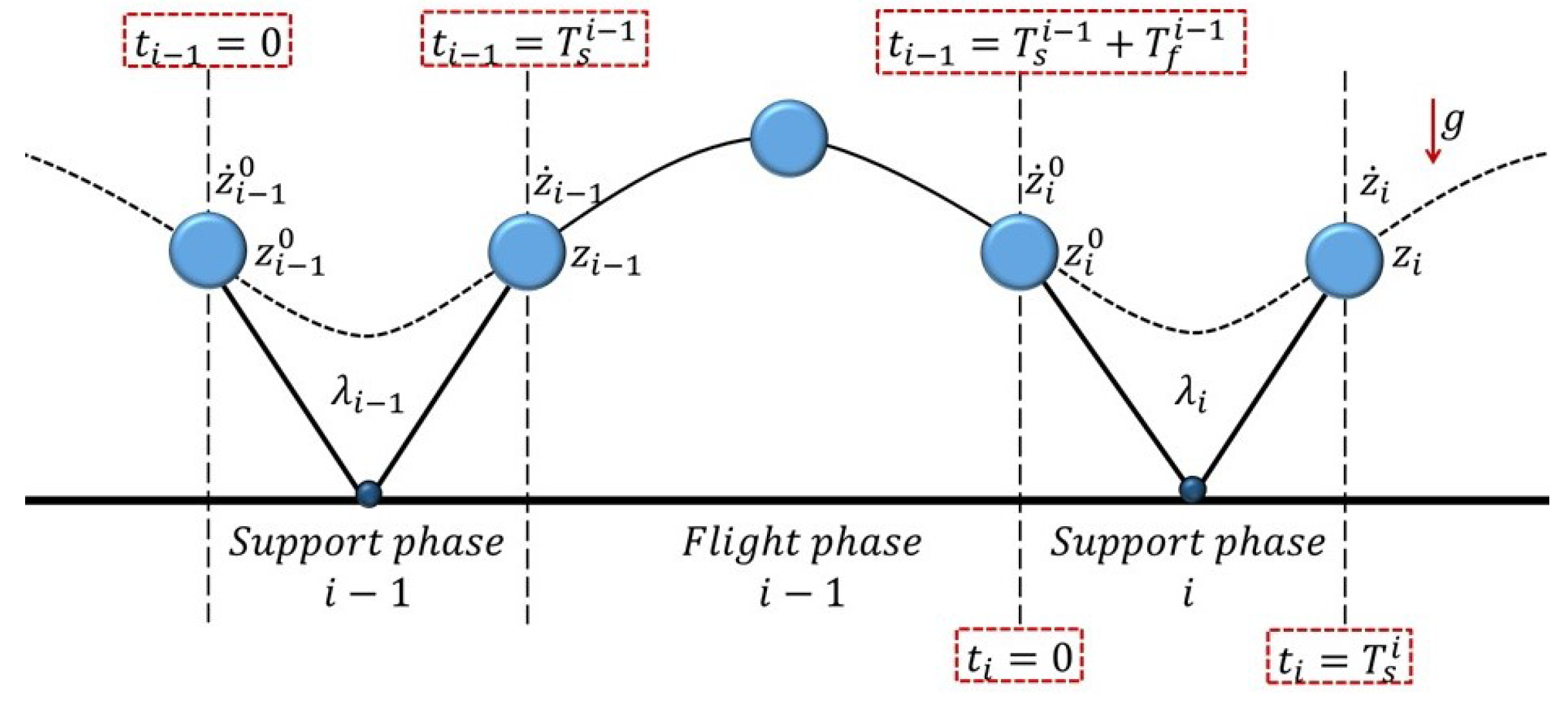
3. Placement of Landing Foot

The ZMP is related to motion stability, and it should stay within the sole of the supporting foot. Besides, it also affects the horizontal acceleration and deceleration of the biped robot. Equation (3) indicates that with the COM ahead of the ZMP, i.e., $x>x_{ZMP}$, the biped robot is accelerated and that with the ZMP ahead of the COM, it is decelerated. This means that the speed of the robot can be controlled by changing the relative horizontal position of the COM with respect to the ZMP.

In this paper, the relative position of the COM with respect to the ZMP of the landing foot is determined for desired motion in the horizontal direction. For this, let’s assume that the ZMP in a support phase is located at the center of the supporting foot, i.e., $x_{ZMP}=0$. Then, Equation (3) becomes

$$\begin{array}{ccc}\hfill {\ddot{x}}_i\left(t_i\right)& =& {\lambda }_i^2{x}_i\left(t_i\right),(0\le t_i\le T_s^i).\hfill \end{array}$$

(8)

Because ${\lambda }_i$ is constant during support phase i, the solution to Equation (8) with initial conditions of $x_i\left(0\right)=x_i^0$ and ${\dot{x}}_i\left(0\right)={\dot{x}}_i^0$ is

$$\begin{array}{ccc}\hfill x_i\left(t_i\right)& =& B_x^i{e}^{{\lambda }_i{t}_i}+C_x^i{e}^{-{\lambda }_i{t}_i},(0\le t_i\le T_s^i),\hfill \end{array}$$

(9)

and thus

$$\begin{array}{c}\hfill {\dot{x}}_i\left(t_i\right)={\lambda }_i(B_x^i{e}^{{\lambda }_i{t}_i}-C_x^i{e}^{-{\lambda }_i{t}_i}),(0\le t_i\le T_s^i),\end{array}$$

(10)

where

$$\begin{array}{ccc}\hfill B_x^i& =& \frac{1}{2}\left(x_i^0+\frac{{\dot{x}}_i^0}{{\lambda }_i}\right),\hfill \\ \hfill C_x^i& =& \frac{1}{2}\left(x_i^0-\frac{{\dot{x}}_i^0}{{\lambda }_i}\right).\hfill \end{array}$$

Note that the initial horizontal velocity at the support phase i, i.e., ${\dot{x}}_i^0$, should be equal to that at the end of support phase $i-1$ since it is assumed that there is no horizontal force applied at the robot during flight phase $i-1$.

The initial position of the COM with respect to the supporting foot, i.e., $x_i^0$, is computed based on desired horizontal motion in the support phase i. Suppose there is the desired horizontal speed at the end of support phase i, i.e., ${\dot{x}}_i\left(T_s^i\right)=V_{x,d}^i$, the initial position of the COM for the desired horizontal motion is computed from Equation (10) as

$$\begin{array}{c}\hfill x_i^0=\frac{2V_{x,d}^i{e}^{{\lambda }_i{T}_s^i}-{\dot{x}}_i^0\left(e^{2{\lambda }_i{T}_s^i}+1\right)}{{\lambda }_i\left(e^{2{\lambda }_i{T}_s^i}-1\right)}.\end{array}$$

(11)

If the horizontal speed does not reach the desired at the end of the support phase i, i.e., ${\dot{x}}_i\left(T_s^i\right)\ne V_{x,d}^i$, the initial COM position of the next support phase, $x_{i+1}^0$, is computed to reach the desired velocity in the next support phase based on Equation (11).

In this paper, $x_i^0\ne -x_i\left(T_s^i\right)$, and thus the generated trajectory is asymmetric, which may cause the robot to exceed its workspace. In order to prevent this, the desired horizontal speed of the support phase should be limited. So, suppose there exists a limit in $x_i\left(T_s^i\right)$, ${\overline{x}}_i$, noting that $x_i\left(t_i\right)$ keeps increasing near the end of the support phase. Then,

$$\begin{array}{c}\hfill x_i\left(T_s^i\right)=B_x^i{e}^{{\lambda }_i{T}_s^i}+C_x^i{e}^{-{\lambda }_i{T}_s^i}\le {\overline{x}}_i,\end{array}$$

(12)

and thus

$$\begin{array}{c}\hfill x_i^0\le \frac{2{\overline{x}}_i{e}^{{\lambda }_i{T}_s^i}}{e^{2{\lambda }_i{T}_s^i}+1}+\frac{{\dot{x}}_i^0}{{\lambda }_i}.\end{array}$$

(13)

From Equations (11) and (13), the constraint to the speed due to the limited workspace of the biped robot is obtained:

$$\begin{array}{c}\hfill V_{x,d}^i\le V_{x,max}^i\triangleq \frac{{\lambda }_i\left(e^{2{\lambda }_i{T}_s^i}-1\right)}{e^{2{\lambda }_i{T}_s^i}+1}{\overline{x}}_i+{\dot{x}}_i^0{e}^{{\lambda }_i{T}_s^i},\end{array}$$

(14)

where $V_{x,max}^i$ denotes the maximum speed that the biped robot can have at the end of the support phase i. With $V_{x,d}^i$ satisfies the constraint, $x_i^0$ can be computed by using Equation (11). However, if the constraint is not satisfied, $V_{x,max}^i$ replaces $V_{x,d}^i$ in computing $x_i^0$. Then $x_{i+1}^0$ is computed to reach the desired velocity in the next support phase.

In this paper, ${\lambda }_i$ and foot placement, $x_i^0$, in the support phase i, is calculated from Equations (7) and (11) based on foot-landing conditions and desired motion and period set by the user, as shown in Figure 3. The computed $x_i^0$ and ${\lambda }_i$ are applied to hierarchical motion control, and desired angle of each joint is generated based on the state of the robot which can be obtained based on kinematics. After the support phase i, the foot placement and ${\lambda }_{i+1}$ for the next support phase are computed based on the desired motion in the next support phase. How to generate the running motion of a biped robot based on hierarchical motion control is introduced in the next section.

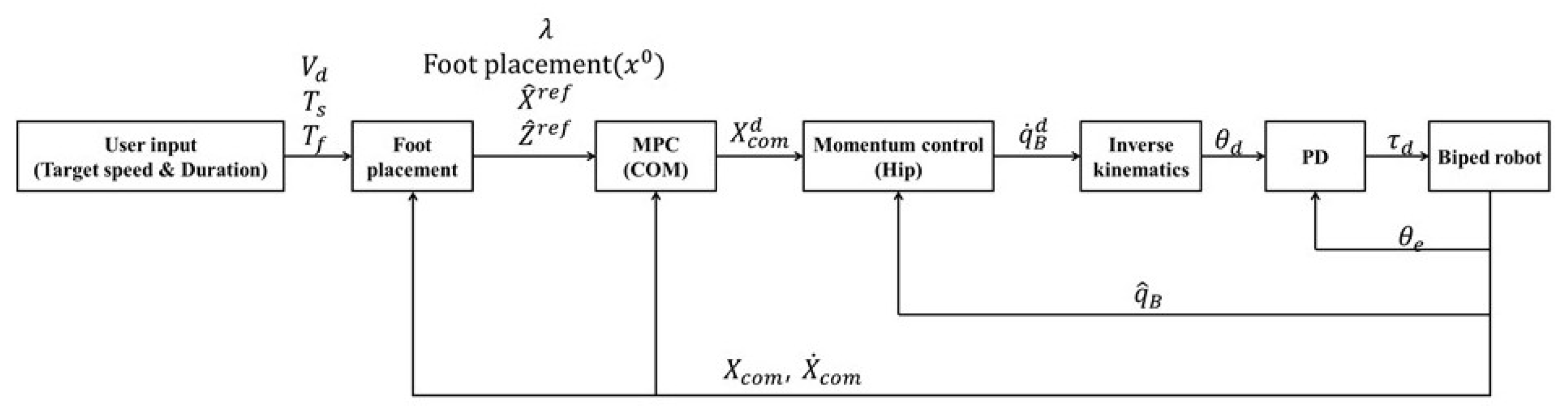
4. Hierarchical Motion Control

For stable locomotion of a biped robot, motion control with constraints for stability, workspace, etc. is needed. MPC is one of the most successful control strategies, which reflects constraints and the actual state of the dynamic system based on the model-based prediction. This paper presents a method to generate stable running motion based on MPC. The proposed method consists of two parts. In the first stage, the trajectory of the COM is generated based on linear MPC with the constraint for stability using a friction cone. In the second stage, a momentum controller based on QP with kinematic constraints on the workspace is applied to make the robot follow the generated COM trajectory.

4.1. COM Trajectory Generation Based on MPC

To generate a COM trajectory, the D-LIPM in Section 2 is used. The position and velocity of the COM are used as the states, and the acceleration is used as the control input. The vertical and horizontal dynamic models of the COM are expressed based on the relation between position, velocity, and acceleration in discrete time as follows

$$\begin{array}{ccc}\hfill \widehat{z}(k+1)& =& A\widehat{z}\left(k\right)+B{u}_z\left(k\right),\hfill \end{array}$$

(15)

$$\begin{array}{ccc}\hfill \widehat{x}(k+1)& =& A\widehat{x}\left(k\right)+B{u}_x\left(k\right),\hfill \end{array}$$

(16)

where

$$\begin{array}{ccc}\hfill \widehat{z}\left(k\right)& =& \left[\begin{array}{c}z\left(k\right)\\ \dot{z}\left(k\right)\end{array}\right],\hfill \\ \hfill \widehat{x}\left(k\right)& =& \left[\begin{array}{c}x\left(k\right)\\ \dot{x}\left(k\right)\end{array}\right],\hfill \\ \hfill A& =& \left[\begin{array}{cc}1& T\\ 0& 1\end{array}\right],\hfill \\ \hfill B& =& \left[\begin{array}{c}\frac{T^2}{2}\\ T\end{array}\right],\hfill \end{array}$$

and constant T denotes the computation step-time interval. Here, $u_x\left(k\right)$ and $u_z\left(k\right)$ are the accelerations in the horizontal and vertical directions. By using the predict models, the states of a biped robot in the prediction horizon of $NT$ can be expressed respectively [37]:

$$\begin{array}{ccc}\hfill \widehat{Z}(k+1)& =& \left[\begin{array}{c}\widehat{z}(k+1)\\ ⋮\\ \widehat{z}(k+N)\end{array}\right]=\widehat{A}\widehat{z}\left(k\right)+\widehat{B}{U}_z\in {\mathbb{R}}^{2N},\hfill \end{array}$$

(17)

$$\begin{array}{ccc}\hfill \widehat{X}(k+1)& =& \left[\begin{array}{c}\widehat{x}(k+1)\\ ⋮\\ \widehat{x}(k+N)\end{array}\right]=\widehat{A}\widehat{x}\left(k\right)+\widehat{B}{U}_x\in {\mathbb{R}}^{2N},\hfill \end{array}$$

(18)

$$\begin{array}{ccc}\hfill {\widehat{Z}}_P(k+1)& =& \left[\begin{array}{c}z(k+1)\\ ⋮\\ z(k+N)\end{array}\right]={\widehat{S}}_P\widehat{Z}(k+1)\in {\mathbb{R}}^N,\hfill \end{array}$$

(19)

$$\begin{array}{ccc}\hfill {\widehat{X}}_P(k+1)& =& \left[\begin{array}{c}x(k+1)\\ ⋮\\ x(k+N)\end{array}\right]={\widehat{S}}_P\widehat{X}(k+1)\in {\mathbb{R}}^N,\hfill \end{array}$$

(20)

where

$$\begin{array}{ccc}\hfill U_x& =& {\left[\begin{array}{ccc}{u}_x\left(k\right)& u_x(k+1)\cdots & u_x(k+N-1)\end{array}\right]}^T\in {\mathbb{R}}^N,\hfill \\ \hfill U_z& =& {\left[\begin{array}{ccc}{u}_z\left(k\right)& u_z(k+1)\cdots & u_z(k+N-1)\end{array}\right]}^T\in {\mathbb{R}}^N,\hfill \\ \hfill \widehat{A}& =& {\left[\begin{array}{ccc}A& A^2\cdots & A^N\end{array}\right]}^T\in {\mathbb{R}}^{2N\times 2},\hfill \\ \hfill \widehat{B}& =& \left[\begin{array}{ccc}B& 0\cdots & 0\\ AB& B\cdots & 0\\ ⋮& ⋮\ddots & 0\\ A^{N-1}B& A^{N-2}B\cdots & B\end{array}\right]\in {\mathbb{R}}^{2N\times N},\hfill \\ \hfill C& =& \left[\begin{array}{cc}1& 0\end{array}\right],\hfill \\ \hfill {\widehat{S}}_P& =& \left[\begin{array}{ccc}C& 0\cdots & 0\\ 0& C\cdots & 0\\ ⋮& ⋮\ddots & 0\\ 0& 0\cdots & C\end{array}\right]\in {\mathbb{R}}^{N\times 2N}.\hfill \end{array}$$

The objective function of the vertical motion is defined to follow the reference position and velocity of the COM and keep the $\lambda$ to the calculated reference value based on Equation (4). The minimized problem for vertical motion can be expressed as

$$\begin{array}{ccc}\hfill \underset{U_z}{min}{\alpha }_{COM}^Z\left|\right|U_z{\left|\right|}^2& +& {\beta }_{COM}^Z\left|\right|{\widehat{Z}}^{ref}-\widehat{Z}(k+1){\left|\right|}^2\hfill \\ & +& {\gamma }_{COM}^Z\left|\right|U_z+\overline{g}-{\lambda }^2{\widehat{Z}}_P(k+1){\left|\right|}^2,\hfill \end{array}$$

(21)

where ${\alpha }_{COM}^Z$, ${\beta }_{COM}^Z$ and ${\gamma }_{COM}^Z$ respectively denote the weights of optimization for control input, position, and $\lambda$. $\overline{g}\in {\mathbb{R}}^N$ consists gravitational acceleration, g. ${\widehat{Z}}^{ref}$ denotes reference position and speed in the vertical direction at the end of each support phase, i.e., $t_i=T_s^i$, which can be calculated based on Equations (5) and (6) with calculated $\lambda$.

Because the GRF in the vertical direction, $F_z\triangleq m(U_z+\overline{g})$, must be positive value in the support phase [26], the contact force in the vertical direction is constrained:

$$\begin{array}{c}\hfill 0\le m(U_z+\overline{g})\le m(U_{z,max}+\overline{g}),\end{array}$$

(22)

where m denotes the total mass of the biped robot; $U_{z,max}$ denotes maximum acceleration in the vertical direction which is applied to constraint $F_z$ within the desired range set by the user. This optimization problem can be expressed as a canonical quadratic problem:

$$\begin{array}{c}\hfill \underset{U_z}{min}\frac{1}{2}{U}_z^T{Q}_z{U}_z+P_z^T{U}_z,\end{array}$$

(23)

subject to

$$\begin{array}{c}\hfill {\underline{U}}_z<U_z<{\overline{U}}_z,\end{array}$$

where

$$\begin{array}{ccc}\hfill Q_z& =& {\alpha }_{COM}^Z{I}_N+{\beta }_{COM}^Z{\widehat{B}}^T\widehat{B}+{\gamma }_{COM}^Z{(I_N-{\lambda }^2{\widehat{S}}_P\widehat{B})}^T(I_N-{\lambda }^2{\widehat{S}}_P\widehat{B})\in {\mathbb{R}}^{N\times N},\hfill \\ \hfill P_z& =& {(\widehat{A}\widehat{z}\left(k\right)-{\widehat{Z}}^{ref})}^T\widehat{B}+{(\overline{g}-{\lambda }^2{\widehat{S}}_P\widehat{A}\widehat{z}\left(k\right))}^T(I_N-{\lambda }^2{\widehat{S}}_P\widehat{B})\in {\mathbb{R}}^N,\hfill \\ \hfill {\underline{U}}_z& =& -\overline{g}\in {\mathbb{R}}^N,\hfill \\ \hfill {\overline{U}}_z& =& U_{z,max}\in {\mathbb{R}}^N,\hfill \end{array}$$

$I_N\in {\mathbb{R}}^{N\times N}$ is identity matrix.

The objective function of horizontal motion is designed to follow the reference position and velocity of the COM and keep the ZMP close to the center of the supporting foot for stability based on Equation (8). The minimized problem for horizontal motion can be expressed as

$$\begin{array}{ccc}\hfill \underset{U_x}{min}{\alpha }_{COM}^X\left|\right|U_x{\left|\right|}^2& +& {\beta }_{COM}^X\left|\right|{\widehat{X}}^{ref}-\widehat{X}(k+1){\left|\right|}^2\hfill \\ & +& {\gamma }_{COM}^X\left|\right|U_x-{\lambda }^2{\widehat{X}}_P(k+1){\left|\right|}^2,\hfill \end{array}$$

(24)

where ${\alpha }_{COM}^X$, ${\beta }_{COM}^X$ and ${\gamma }_{COM}^X$ respectively denote the weights of optimization for control input, the position of the COM, and ZMP. ${\widehat{X}}^{ref}$ denotes reference position and speed in the horizontal direction at the end of each support phase, i.e., $t_i=T_s^i$, which can be calculated based on Equations (9) and (10) with calculated foot placement.

For the stable dynamic motion of the COM, constraints based on the friction cone are applied [38]. The contact force in the horizontal plane is constrained to lie in the friction cone defined by

$$\begin{array}{c}\hfill -\overline{\mu }{F}_z<m{U}_x<\overline{\mu }{F}_z,\end{array}$$

(25)

where $\overline{\mu }$ denotes the friction coefficient between the ground and the foot of the robot. These minimized problems can be also expressed as a canonical quadratic form:

$$\begin{array}{c}\hfill \underset{U_x}{min}\frac{1}{2}{U}_x^T{Q}_x{U}_x+P_x^T{U}_x,\end{array}$$

(26)

subject to

$$\begin{array}{c}\hfill {\underline{U}}_x<U_x<{\overline{U}}_x,\end{array}$$

where

$$\begin{array}{ccc}\hfill Q_x& =& {\alpha }_{COM}^{X}E+{\beta }_{COM}^X{\widehat{B}}^T\widehat{B}+{\gamma }_{COM}^X{(I_N-{\lambda }^2{\widehat{S}}_P\widehat{B})}^T(I_N-{\lambda }^2{\widehat{S}}_P\widehat{B})\in {\mathbb{R}}^{N\times N},\hfill \\ \hfill P_x& =& {(\widehat{A}\widehat{x}\left(k\right)-{\widehat{X}}^{ref})}^T\widehat{B}+{(-{\lambda }^2{\widehat{S}}_P\widehat{B})}^T(I_N-{\lambda }^2{\widehat{S}}_P\widehat{B})\in {\mathbb{R}}^N,\hfill \\ \hfill {\underline{U}}_x& =& -\overline{\mu }\frac{F_z}{m}\in {\mathbb{R}}^N,\hfill \\ \hfill {\overline{U}}_x& =& \overline{\mu }\frac{F_z}{m}\in {\mathbb{R}}^N.\hfill \end{array}$$

From the object functions, the control inputs in the horizontal and vertical direction, i.e., $U_x$ and $U_z$, are obtained, which are used to generate the COM trajectory of the biped robot based on Equations (17) and (18).

Typically, a biped robot has several joints, and the motion of each joint affects its COM. To follow the generated COM trajectories, for this reason, trajectory generation of the joints which realize the desired COM trajectory is needed [18,26,39]. To generate the trajectory of joints to follow the COM trajectory, in this paper, momentum control is applied, which is presented in Section 4.2.

4.2. Momentum Control Based on Optimization

In this paper, a QP-based momentum control, taking into account the constraints of the workspace, is proposed to follow the desired COM trajectory. When the floating-base of the biped robot has n degree-of-freedom (DOF), as shown in Figure 4, its linear and angular momentum, $\widehat{K}$ and $\widehat{H}$, are described by

$$\begin{array}{c}\hfill \widehat{L}\triangleq \left[\begin{array}{c}\widehat{K}\\ \widehat{H}\end{array}\right]=M_B(q_B,\theta ){\dot{q}}_B+H_{\theta }\dot{\theta },\end{array}$$

(27)

where $q_B\triangleq {\left[q_l^T{q}_a^T\right]}^T\in {\mathbb{R}}^n$ is the position and orientation vector of the hip link with respect to the supporting foot; $q_l$ and $q_a$ are respectively the position and orientation of the hip link; $\theta$ denotes the joint angle of the arms and legs; $\widehat{K}$ and $\widehat{H}$ are respectively the linear and angular momentum of the robot; and $M_B$ and $H_{\theta }$ are the inertia matrices which indicate how the velocity of hip link and all the joints affect the linear and angular momentum respectively. For the momentum control, the dynamics model is defined based on Equation (27) and the relation between position, velocity, and acceleration in discrete time:

$$\begin{array}{ccc}\hfill {\widehat{q}}_B^{k+1}& =& A{\widehat{q}}_B^k+B{u}_B,\hfill \end{array}$$

(28)

$$\begin{array}{ccc}\hfill {\widehat{L}}^{k+1}& =& {\widehat{M}}_B{\widehat{q}}_B^{k+1}+H_{\theta }\dot{\theta },\hfill \end{array}$$

(29)

where

$$\begin{array}{ccc}\hfill {\widehat{q}}_B& =& \left[\begin{array}{c}{q}_B^k\\ {\dot{q}}_B^k\end{array}\right]\in {\mathbb{R}}^{2n},\hfill \\ \hfill A& =& \left[\begin{array}{cc}{I}_n& T{I}_n\\ {\mathbf{0}}_{n\times n}& I_n\end{array}\right]\in {\mathbb{R}}^{2n\times 2n},\hfill \\ \hfill B& =& {\left[\begin{array}{cc}\frac{T^2}{2}{I}_n& T{I}_n\end{array}\right]}^T\in {\mathbb{R}}^{2n\times 2},\hfill \\ \hfill {\widehat{M}}_B& =& \left[\begin{array}{cc}{\mathbf{0}}_{n\times n}& M_B\end{array}\right]\in {\mathbb{R}}^{n\times 2n},\hfill \end{array}$$

${\mathbf{0}}_{n\times n}$ and $I_n$ denote $n\times n$ zero and identity matrix, respectively; $u_B\in {\mathbb{R}}^n$ denotes the acceleration of the hip link; and T denotes the sampling time of the controller. By using the dynamic model, the optimization problem is formulated as

$$\begin{array}{c}\hfill \underset{u_B}{min}{\alpha }_B^L\left|\right|u_B{\left|\right|}^2+{\beta }_B^L\left|\right|{\widehat{q}}_B^{ref}-{\widehat{q}}_B^{k+1}{\left|\right|}^2+{\gamma }_B^L\left|\right|{\widehat{L}}^{ref}-{\widehat{L}}^{k+1}{\left|\right|}^2,\end{array}$$

(30)

where ${\alpha }_B^L$, ${\beta }_B^L$ and ${\gamma }_B^L$ are the weights. Typically, weights in many optimization problems are constant [23,26,31]. However, for ${\gamma }_B^L$, a variable weight with respect to the velocity of the biped robot is used instead:

$$\begin{array}{c}\hfill {\gamma }_B^L={\gamma }_B\left|\right|1+\rho {\dot{x}}_{COM}\left|\right|,\end{array}$$

(31)

where ${\gamma }_B$ is its initial weight for momentum; ${\dot{x}}_{com}$ is the actual horizontal velocity of the biped robot; and $\rho$ is a constant scale factor for the velocity of the robot. With this, the effect of the actual velocity of the robot is reflected in the momentum control. The optimization problem for momentum control, i.e., Equation (30), can be expressed as a canonical quadratic problem as

$$\begin{array}{c}\hfill \underset{u_B}{min}\frac{1}{2}{u}_B^T{Q}_B{u}_B+P_B^T{u}_B,\end{array}$$

(32)

subject to

$$\begin{array}{c}\hfill {\widehat{q}}_l<{\widehat{q}}_B^{k+1}<{\widehat{q}}_u\end{array}$$

where

$$\begin{array}{ccc}\hfill Q_B& =& {\alpha }_B^{L}E+{\beta }_B^L{\widehat{B}}^T\widehat{B}+{\gamma }_B^L{\left({\widehat{M}}_B\widehat{B}\right)}^T\left({\widehat{M}}_B\widehat{B}\right),\hfill \\ \hfill P_B& =& {(\widehat{A}{\widehat{q}}_B-{\widehat{q}}_B^{ref})}^T\widehat{B}+{({\widehat{M}}_B\widehat{A}{\widehat{q}}_B-{\widehat{L}}^{ref}+H_{\theta }\dot{\theta })}^T\left({\widehat{M}}_B\widehat{B}\right),\hfill \end{array}$$

where ${\widehat{L}}^{ref}\triangleq {\left[K^{ref}{H}^{ref}\right]}^T$ denotes reference momentum with $K^{ref}$ and $H^{ref}$ respectively denoting the linear and angular reference momentum; and ${\widehat{q}}_u$ and ${\widehat{q}}_l$ respectively denote upper and lower boundary of workspace.

Here, the reference momentum is generated based on the COM trajectory and reference angular motion of the hip link:

$$\begin{array}{ccc}\hfill {\widehat{K}}^{ref}& =& m{\dot{X}}_{com}^d,\hfill \end{array}$$

(33)

$$\begin{array}{ccc}\hfill {\widehat{H}}^{ref}& =& I_B{\dot{q}}_a^d,\hfill \end{array}$$

(34)

where m denotes the total mass of the biped robot; $I_B$ denotes the inertia of the hip link; ${\dot{X}}_{com}^d\triangleq {\left[{\dot{x}}^d{\dot{z}}^d\right]}^T$ is desired velocity of the COM generated in the first stage of the proposed method; $q_a^d$ is desired angular trajectory of the hip link. The desired angular motion of the hip link is generated based on the PD scheme:

$$\begin{array}{c}\hfill {\dot{q}}_a^d=P_a(q_a^{ref}-q_a)+D_a({\dot{q}}_a^{ref}-{\dot{q}}_a),\end{array}$$

(35)

where $q_a^{ref}$ and ${\dot{q}}_a^{ref}$ are reference orientation and angular velocities of the hip link, respectively; $P_a$ and $D_a$ are proportional and derivative gain, respectively. By minimizing the object functions with the reference momentum, the control input of the hip link, $u_B$, is obtained, and the desired trajectory of the hip link is computed based on Equation (28).

Figure 5 describes the block diagram for proposed methods. First, $\lambda$ and foot placement is computed based on the periods, $T_s$ and $T_f$, and desired velocity, $V_d\triangleq {\left[V_{x,d}{V}_{z,d}\right]}^T$, set by the user. Based on $\lambda$ and the foot placement, the reference position of the COM for each support phase, i.e., ${\widehat{X}}^{ref}$ and ${\widehat{Z}}^{ref}$, are computed. Then, a running trajectory is generated based on the proposed MPC, where the trajectory of COM, $X_{COM}^d$, is generated based on linear MPC with its states, $X_{COM}\triangleq {\left[xz\right]}^T$, and stability constraints using a friction cone. Then, the computed COM trajectory is used as the input to QP based momentum controller as a reference momentum, where the trajectory of the hip link, $q_B^d$, is computed based on its state, ${\widehat{q}}_B$. From the generated trajectory of the hip link and foot, the trajectory of each joint, ${\theta }_d$, is obtained by inverse kinematics, A PD controller generates the input torque for each joint, ${\tau }_d$.

5. Performance Validation

To show the effectiveness of the proposed methods and at the same time to measure their performance, computer simulations of the running of a biped robot were performed in a 2-dimensional environment. For the simulations, Mathworks’ Matlab and a commercial dynamics simulator called RecurDyn were used. The latter offers various kinds of contact models, joints, force, and dynamic modeling tools such as link length, mass, geometrical constraints, etc., and has the advantage of convenience to execute simulations without developing mathematical dynamic equations.

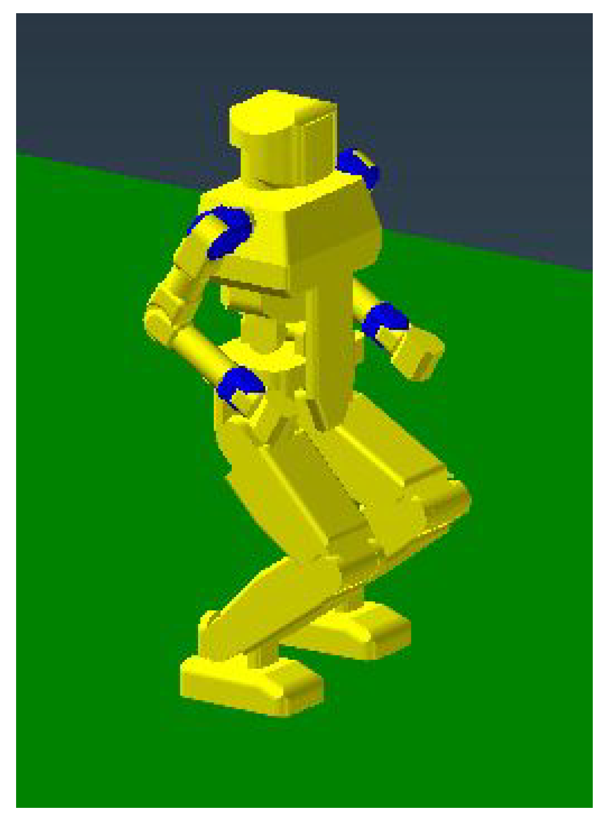
5.1. Simulation Environment

A simulation model based on our biped robot called HYBRO (Hanyang Biped Robot) is created as shown in Figure 6. The total weight of the robot model was about 33 kg and the weight of the upper body including the arms was about 18 kg. The height of the robot was 1.15 m and the height of the hip was 0.625 m. All of its parameters computed from CAD data of HYBRO are summarized in

Table 1. Robot parameters.

Parts	Mass (kg)	Height/Length (m)
Hip	18.01
Thigh (2EA)	2.93	0.265
Shank (2EA)	2.75	0.265
Foot (2EA)	1.93	0.1
Total	33.32	0.625

. This model has 28 DOFs; however, just 6 DOFs of the lower body were used and other joints were fixed for the simulations in a 2D environment.

A model of contact between the supporting foot and the ground is very important for more realistic simulations. In this paper, the Hunt–Crossley model was used [40], where the vertical component of the GRF was computed by

$$F_n=k{\delta }^{m1}+c\frac{\dot{\delta }}{\left|\delta \right|}{\left|\dot{\delta }\right|}^{m_2}{\delta }^{m_3},$$

(36)

where k and c denote the spring and damping coefficients, respectively; $\delta$ denotes the amount of deformation at the foot on the ground; and $m_1$, $m_2$ and $m_3$ respectively denote the stiffness, damping, and indentation exponents. The horizontal component of the contact force was calculated as

$$\begin{array}{ccc}\hfill F_f& =& \mu \left(\nu \right)|F_n|,\hfill \end{array}$$

(37)

where $\mu \left(\nu \right)$ is the friction coefficient depending on slip velocity, $\nu$. The coefficient is calculated based on the offered friction model by RecurDyn [41,42] with ${\nu }_s$, ${\nu }_d$, ${\mu }_s$, and ${\mu }_d$, where ${\nu }_s$ and ${\nu }_d$ are respectively the static and dynamic threshold velocities; and ${\mu }_s$ and ${\mu }_d$ respectively denote the static and dynamic friction coefficients. The numerical values of all these parameters used in the simulations are summarized in

Table 2. Friction parameters.

Symbols	Values	Unit	Symbols	Values	Unit
k	2000	kN/m	${\mu }_d$	0.8	-
c	1.0	kNs/m	${\mu }_s$	1.0	-
$m_1$	1.3	-	${\nu }_d$	0.15	m/s
$m_2$	1.0	-	${\nu }_s$	0.1	m/s
$m_3$	2.0	-

.

To verify the performance of the proposed algorithm, simulations of the running of a biped robot in several different environments were carried out. Firstly, the biped robot running on flat terrain was simulated to show that the velocity of the robot was controlled well with the proposed method. Secondly, to confirm the adaptability to the uncertainties in the environment, simulations for running on unobserved uneven terrains were performed.

All the simulations used an identical scenario as follows. Firstly, the robot bent its knees 55 degrees to avoid kinetic singularity at $t=1.1$ s, such that the hip was located at 0.4 m from the ground and the forward lean angle of the upper body was 7.5 degrees. Afterward, the robot started running to reach the target speed. Until $t=1.8$ s, the reference speed in the horizontal direction of the support phase is 0 m/s, afterwards, it is increased gradually to the target speed.

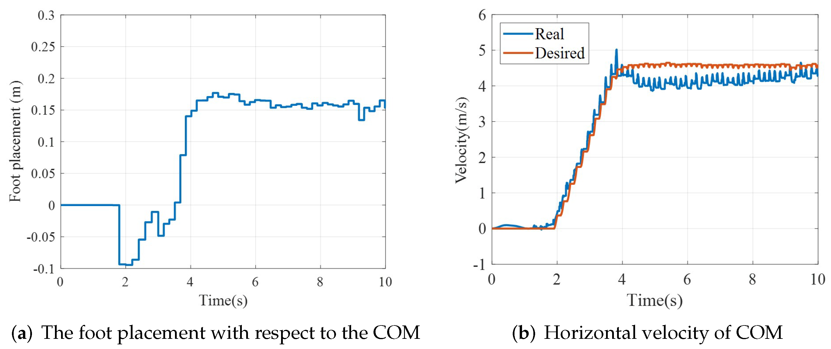
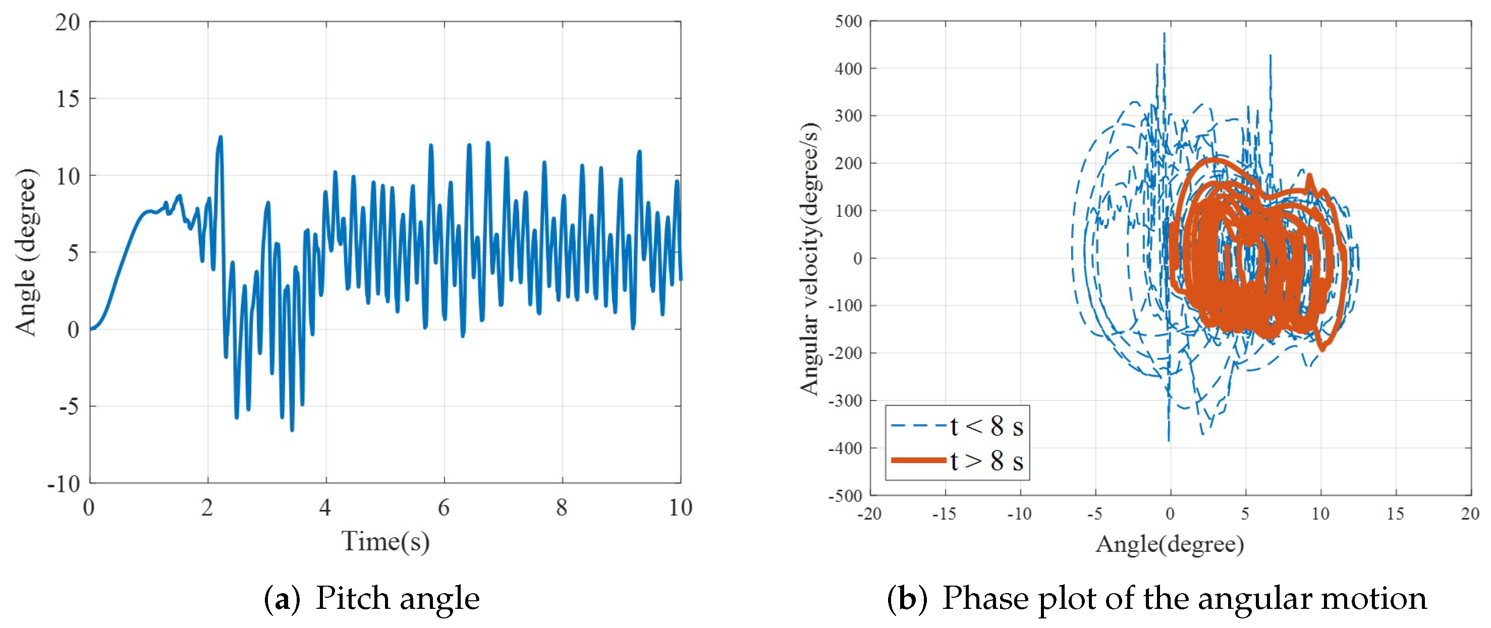
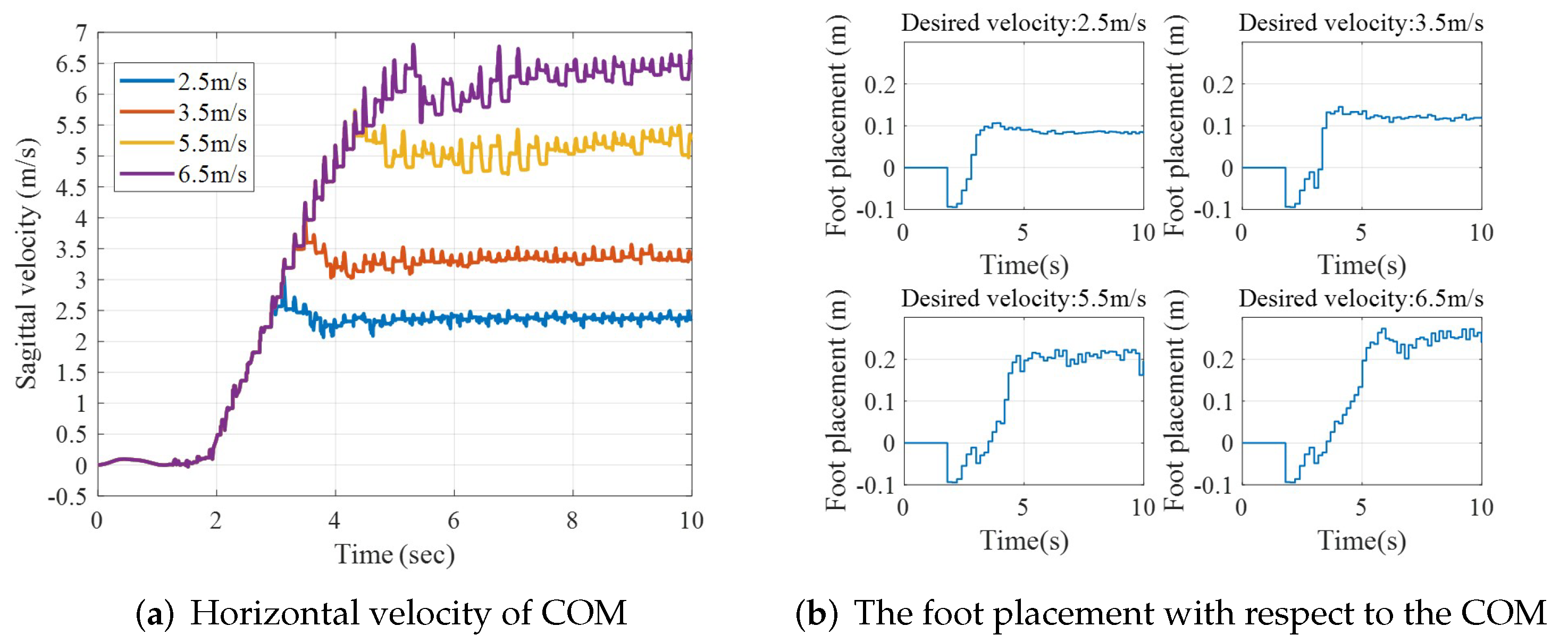
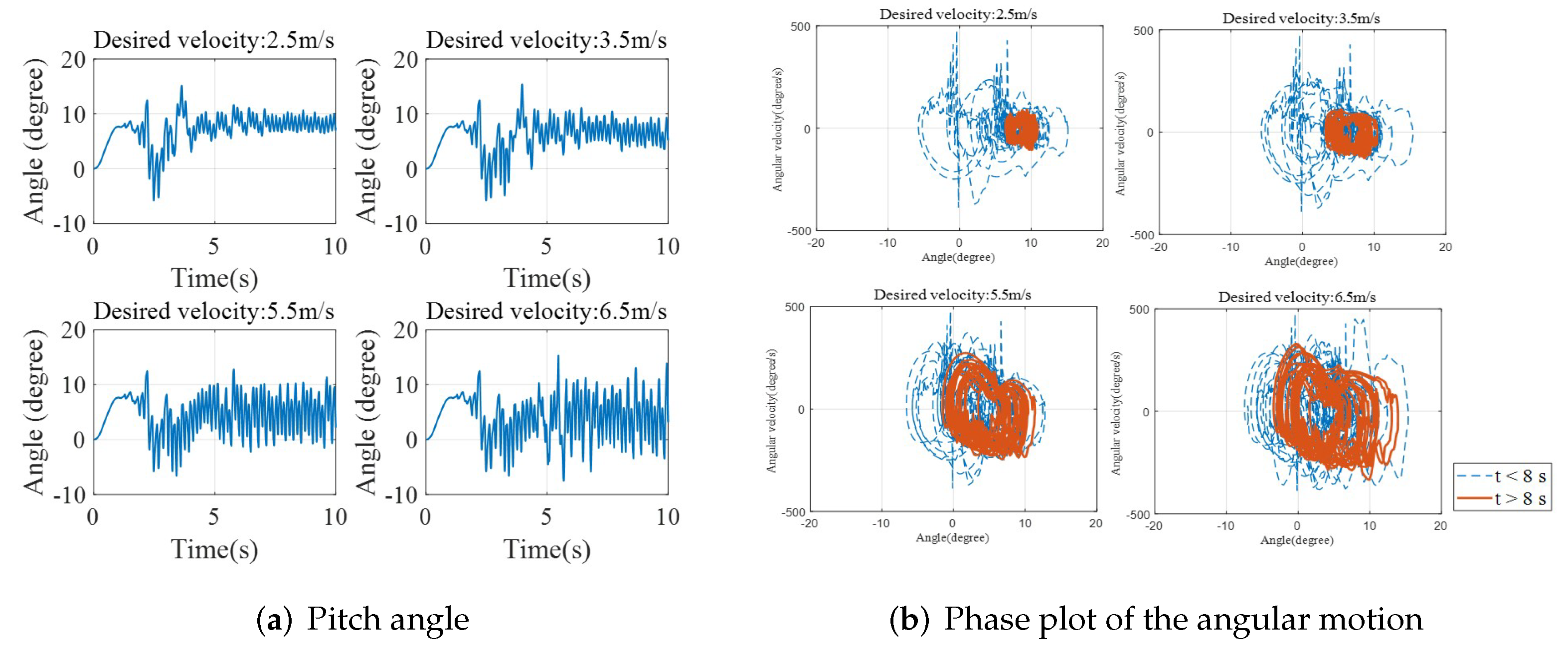
5.2. Running on Flat Terrain

Simulations of the biped robot running on a flat terrain were performed. The duration of the support phase, $T_s$, was initially set at 0.1 s and it was gradually decreased to 0.07, 0.065, and 0.060 s as the robot sped up. The duration of the flight phase, $T_f$, remained constant at 0.1 s in all runs. Before the robot started running, it bent its knees such that making the COM located 0.4469 m from the ground, which was used as $Z^{ref}$.

Table 3. Duration of support phase.

${\mathit{T}}_{\mathit{s}}$	Simulation Time	$\mathit{\lambda }$
0.100 s	1.10 s∼3.00 s	6.69
0.070 s	3.00 s∼4.02 s	7.35
0.065 s	4.02 s∼5.34 s	7.51
0.060 s	5.34 s∼10.00 s	7.69

shows how $T_s$ and $\lambda$ changed in a simulation.

The control parameters used in the simulations, such as the weights and parameters for constraints of MPC and momentum control, were listed in

Table 4. Control parameters.

Symbols	Description	Value
${\alpha }_{COM}^X$	Weight of MPC for control input in the horizontal direction	1.0
${\beta }_{COM}^X$	Weight of MPC for speed in the horizontal direction	$2.9\times {10}^7$
${\gamma }_{COM}^X$	Weight of MPC for ZMP	$1.1\times {10}^{11}$
${\alpha }_{COM}^Z$	Weight of MPC for control input in the vertical direction	1.0
${\beta }_{COM}^Z$	Weight of MPC for speed in the vertical direction	$3.9\times {10}^7$
${\gamma }_{COM}^Z$	Weight of MPC for $\lambda$	$1.2\times {10}^{11}$
$\overline{\mu }$	Friction coefficient for friction cone of MPC	$0.65$
${\alpha }_B^L$	Weight of momentum control for control input	$1.0$
${\beta }_{B,l}^L$	Weight of momentum control for position of linear motion	$0.0$
${\gamma }_{B,l}^L$	Weight of momentum control for linear momentum	$4.7\times {10}^7$
${\beta }_{B,a}^L$	Weight of momentum control for angle of angular motion	$7.6\times {10}^7$
${\gamma }_{B,a}^L$	Weight of momentum control for angular momentum	$2.2\times {10}^4$
${\rho }_l$	Scale factor of variable weight for linear momentum	$0.1$
${\rho }_a$	Scale factor of variable weight for angular momentum	$0.1$

.

To measure the running speed relative to the size of the robot, Froude number ($F_r$), a dimensionless number defined by

$$\begin{array}{c}\hfill F_r=\frac{v^2}{gl},\end{array}$$

was often used (e.g., Refs. [43,44,45]), where v is the speed of the robot and l is the leg length. Five simulations were carried out, each with a different target speed: 2.5 m/s ($F_r=1.0194$), 3.5 m/s ($F_r=1.9980$), 4.5 m/s ($F_r=3.3028$), 5.5 m/s ($F_r=4.9337$) and 6.5 m/s ($F_r=6.8909$).

Figure 7a shows how the foot placement relative to the hip changed when the target speed was 4.5 m/s. Companying this with Figure 7b, it is clear that the size of the footstep gradually increased as the speed of the robot increased in $1.8\le t\le 4$, and finally settled around 0.15 m. The speed of the robot closely tracked the desired at 4.5 m/s as shown in Figure 7b.

The angular motion of the upper body was generated based on momentum control. Figure 8a shows how the pitch angle of the hip changed. During 1.8 s $<t<$ 4 s, the robot’s upper body leaned backward 5 degrees due to the body acceleration. However, after reaching the target speed, 4.5 m/s, the body leaned forward at an angle between 0 and 15 degrees. Figure 8b shows the phase plot for the angle and angular velocity of the upper body, where the dotted line represents the region of the speed increase, and the solid line represents the region of a constant speed. In this figure, it can be confirmed that the pitch motion did not deviate from a certain range. From Figure 7b and Figure 8b, it was also shown that the motion of the biped robot was well controlled for stable running with the use of the proposed method, and the robot tracked the desired speed without any fails.

Figure 9 shows how the robot ran with different target speeds summarized in

Table 5. Simulation results for running in various target velocity.

Target Velocity	Foot Placement	Velocity	${\mathit{F}}_{\mathit{r}}$
2.5 m/s	0.085 m	2.49 m/s	1.0162
3.5 m/s	0.119 m	3.55 m/s	2.0659
5.5 m/s	0.214 m	5.49 m/s	4.9195
6.5 m/s	0.263 m	6.70 m/s	7.3185

.

When the desired velocity was 2.5 m/s, the foot placement was settled at 0.085 m. The foot placement relative to the hip increased as the target speed increased, and became 0.263 m when the target speed was 6.5 m/s. This result confirms that the speed of the robot changed depending on the foot placement, and that the speed of the robot was controlled by proper foot placement. Because the stride changed according to the speed of the biped robot, the trajectory of the swing leg changed, and the upper body motion also changed to compensate for the angular momentum change due to the swing leg. At low speeds, the scale of the swing leg moved slowly for short strides, and the motion of the upper body was also small to compensate for this. On the other hand, when the speed increased, the velocity of the swing leg also increased, and the motion of the upper body for momentum compensation also increased. Figure 10 shows the angle of the upper body and the phase plot of the angular motion for each target speed. In the case of low target speed, the range of motion of the upper body was small and so was the range of the phase plot. When the target speed increased, the motion of the upper body also increased. However, it did not deviate from a certain range. Companying this with Figure 9a, it was confirmed that the motion of the biped robot was well controlled and the robot tracked each desired speed without any fails with the proposed method.

5.3. Running on Uneven Terrain: Case 1

To show the adaptability of the robot to various uncertainties in the environment, simulations of running on shallow stairs shown in Figure 11 were carried out. The elevation of each stair was 30 mm, so the level of stair H was 240 mm from the ground. The highest level was 6 m-long, and then there were downhill stairs to the level 30 mm from the ground. The heights of all the obstacles are listed in

Table 6. The heights of the obstacles.

Symbols	Height (mm)	Symbols	Height (mm)	Symbols	Height (mm)
A	30	F	180	K	150
B	60	G	210	L	120
C	90	H	240	M	90
D	120	I	210	N	60
E	150	J	180	O	30

.

The targeted running speed was 6.5 m/s. Figure 12a shows the trajectory of the COM and feet in the vertical direction. The foot-landing positions were changed due to the differences in the heights of the obstacles. Despite this, the posture of the robot was controlled well based on the proposed method, and the biped robot passed through obstacles without falling. And the running speed gradually increased up to the target speed, 6.5 m/s, as shown in Figure 12b.

5.4. Running on Uneven Terrain: Case 2

In this simulation, unobserved obstacles with different heights were randomly placed as shown in Figure 13. The left and right feet were raised such that only on a flat part of obstacles, whose level is randomly selected. The height of the obstacles has two cases: 30 mm (Orange) and 60 mm (Blue). The maximum variation in the level of the obstacles was 60 mm, requiring about 10 % of leg length.

Again, the targeted running speed of running was 6.5 m/s. Figure 14a shows the trajectory of the COM and foot in the vertical direction. The foot-landing positions were different due to the differences in the heights of the obstacles. Since the variation in the levels of the foot-landing was more significant and irregular than that of case1, the vertical position of the COM fluctuated more, as observed in Figure 14a. Despite this, the posture of the robot was controlled well based on the proposed method, and the biped robot passed through obstacles without falling.

The horizontal motion also fluctuated because of the uncertainty of the environment as shown in Figure 14b. Companying this with Figure 14a, especially, the fluctuating was more significant when the difference in the vertical position of any consecutive foot-landing was large. Despite this, The trajectory of the COM generated based on the MPC and the robot tracked the desired speed as shown in Figure 14b. The speed of the robot successfully reached 6.72 m/s without falling.

5.5. Discussion

Simulations of the running biped robot on various terrain with uncertainties were carried out. The online running motion according to the variation in the levels of the foot-landing was generated based on the proposed methods, and the speed of the robot successfully reached the target speed with overcoming the uncertainty of the environment. In the simulations, $\lambda$ was calculated according to the duration change of the support phase, and the level change of the terrain was not considered. The situations such as fluctuations in the height of terrain can be reflected by desired vertical motion, which is used to calculate the $\lambda$. The online running motion for various environments can be generated by applying the $\lambda$ according to the situation.

6. Conclusions

This paper proposes a method for online motion control of a running biped robot on an uneven terrain based on D-LIPM and hierarchical control which consists of linear MPC and QP-based momentum control. To generate the running motion through linear MPC, D-LIPM, which splits the nonlinear dynamics model of the running biped robot into two linear models, is proposed. The D-LIPM is applied to the proposed hierarchical control, and the online running motion of the robot is generated. In the first stage of the hierarchy, linear MPC with its states and stability constraints based on a friction cone is applied to generate the COM trajectory. In the second stage, QP-based momentum control with constraints on the workspace is applied to follow the generated COM trajectory.

For the performance validation of the proposed methods, simulations were performed in various environments. In the case of flat terrain, it was shown that the bipedal running motion for each desired speed was generated based on the proposed method and the robot ran at the speed of up to 6.70 m/s. In the case of uneven terrain, simulations are carried out in environments that include unobserved obstacles whose maximum height difference between the obstacles was about 10% of the length of its legs. In these simulations, it was shown that the speed of the robot successfully reached the target speed, 6.5 m/s, without falling despite the uncertainty of the environment. From the simulations, it was shown that the proposed method had stability and robustness to environmental uncertainties.

In the near future, additional studies will be carried out on online trajectory generation and control for bipedal running in more diverse 3-dimensional environments and possibly with deformable and slippery terrains.

References

1. Kajita, S.; Tani, K. Study of dynamic biped locomotion on rugged terrain-theory and basic experiment. In Proceedings of the Fifth International Conference on Advanced Robotics’ Robots in Unstructured Environments, Pisa, Italy, 19–22 June 1991. [Google Scholar]
2. Lee, J.H.; Park, J.H. Optimization of Postural Transition Scheme for Quadruped Robots Trotting on Various Surfaces. IEEE Access 2019, 7, 168126–168140. [Google Scholar] [CrossRef]
3. Chen, Z.; Li, J.; Wang, S.; Wang, J.; Ma, L. Flexible gait transition for six wheel-legged robot with unstructured terrains. Robot. Auton. Syst. 2022, 150, 103989. [Google Scholar] [CrossRef]
4. Waldron, K.J. Mobility and controllability characteristics of mobile robotic platforms. In Proceedings of the IEEE International Conference on Robotics and Automation, St. Louis, MO, USA, 25–28 March 1985. [Google Scholar]
5. Kajita, S.; Kanehiro, F.; Kaneko, K.; Yokoi, K.; Hirukawa, H. The 3rd linear inverted pendulum mode: A simple modeling for biped walking pattern generation. In Proceedings of the International Conference on Intelligent Robots and Systems, Maui, HI, USA, 29 October–3 November 2001. [Google Scholar]
6. Park, J.H.; Kim, K.D. Biped robot walking using gravity-compensated inverted pendulum mode and computed torque control. In Proceedings of the International Conference on Advanced Robotics, Leuven, Belgium, 20–20 May 1998. [Google Scholar]
7. Morimoto, J.; Endo, G.; Nakanishi, J.; Cheng, G. A Biologically Inspired Biped Locomotion Strategy for Humanoid Robots: Modulation of Sinusoidal Patterns by a Coupled Oscillator Model. IEEE Trans. Robot. 2008, 24, 1. [Google Scholar] [CrossRef] [Green Version]
8. Shimmyo, S.; Sato, T.; Ohnishi, K. Biped Walking Pattern Generation by Using Preview Control Based on Three-Mass Model. IEEE Trans. Ind. Electron. 2013, 60, 11. [Google Scholar] [CrossRef]
9. Flayols, T.; Prete, O.D.A.D.; Khadiv, M.; Mansard, N.; Righetti, L. Reactive Balance Control for Legged Robots under Visco-Elastic Contacts. Appl. Sci. 2021, 11, 353. [Google Scholar] [CrossRef]
10. Lu, Y.; Gao, J.; Shi, X.; Tian, D.; Liu, Y. Sliding Balance Control of a Point-Foot Biped Robot Based on a Dual-Objective Convergent Equation. Appl. Sci. 2021, 11, 4016. [Google Scholar] [CrossRef]
11. Kamioka, T.; Sugihara, T. Survey on model-based biped motion control for humanoid robots. Adv. Robot. 2020, 34, 21–22. [Google Scholar]
12. Reibert, M.H.; Tello, T.R. Legged robots that balance. IEEE Expert 1986, 1, 4. [Google Scholar] [CrossRef]
13. Hodgins, J.K.; Raibert, M.H. Adjusting Step Length for Rough Terrain Locomotion. IEEE Trans. Robot. Autom. 1991, 7, 3. [Google Scholar] [CrossRef]
14. Saranli, U.; Schwind, W.J.; Koditschek, D.E. Toward the Control of a Multi-Jointed, Monoped Runner. In Proceedings of the International Conference on Advanced Robotics, Leuven, Belgium, 20–20 May 1998. [Google Scholar]
15. Kwon, O.; Park, J.H. Asymmetric trajectory generation and impedance control for running of biped robots. Auton. Robot. 2009, 26, 47–78. [Google Scholar] [CrossRef]
16. Thanh, D.N.; Hayashi, T.; Yamakita, M. High speed running of flat foot Biped robot with Inerter using SLIP. In Proceedings of the IEEE International Conference on Advanced Intelligent Mechatronics, Busan, Korea, 7–11 July 2015. [Google Scholar]
17. Kajita, S.; Nagasaki, T.; Kaneko, K.; Yokoi, K.; Tanie, K. A Running Controller of Humanoid Biped HRP-2LR. In Proceedings of the International Conference on Robotics and Automation, Barcelona, Spain, 18–22 April 2005. [Google Scholar]
18. Kajita, S.; Nagasaki, T.; Kaneko, K.; Hirukawa, H. ZMP-Based Biped Running Control. IEEE Robot. Autom. Mag. 2007, 14, 63–72. [Google Scholar] [CrossRef]
19. Tajima, R.; Honda, D.; Suga, K. Fast running experiments involving a humanoid robot. In Proceedings of the IEEE International Conference on Robotics and Automation, Kobe, Japan, 18 August 2009. [Google Scholar]
20. Kajita, S.; Kanehiro, F.; Kaneko, K.; Fujiwara, K.; Harada, K.; Yokoi, K.; Hirukawa, H. Biped walking pattern generation by using preview control of zero-moment point. In Proceedings of the International Conference on Advanced Robotics, Taipei, Taiwan, 14–19 September 2003. [Google Scholar]
21. Wu, A.; Geyer, H. Highly robust running of articulated bipeds in unobserved terrain. In Proceedings of the IEEE/RSJ International Conference on Intelligent Robots and Systems, Chicago, IL, USA, 14–18 September 2014. [Google Scholar]
22. Nir, O.; Degani, A. Reactive Control for Bipedal Running Over Random Discrete Terrain Under Uncertainty. In Proceedings of the IEEE/RSJ International Conference on Intelligent Robots and Systems (IROS), Prague, Czech Republic, 27 September–1 October 2021. [Google Scholar]
23. Wensing, P.M.; Orin, D.E. High-Speed Humanoid Running Through Control with a 3D-SLIPM Model. In Proceedings of the IEEE/RSJ International Conference on Intelligent Robot and Systems, Tokyo, Japan, 3–7 November 2013. [Google Scholar]
24. Boroujeni, M.G.; Daneshman, E.; Righetti, L.; Khadiv, M. A unified framework for walking and running of bipedal robots. In Proceedings of the International Conference on Advanced Robotics, Ljubljana, Slovenia, 6–10 December 2021. [Google Scholar]
25. Kuindersma, S.; Permenter, F.; Tedrake, R. An Efficiently Solvable Quadratic Program for Stabilizing Dynamic Locomotion. In Proceedings of the International Conference on Robotics and Automation, Hong Kong, China, 31 May–5 June 2014. [Google Scholar]
26. Dai, H.; Valenzuela, A.; Tedrake, R. Whole-body Motion Planning with Centroidal Dynamics and Full Kinematics. In Proceedings of the IEEE-RAS International Conference on Humanoid Robots, Madrid, Spain, 18–20 November 2014. [Google Scholar]
27. Rathod, N.; Bratta, A.; Focchi, M.; Zanon, M.; Villarreal, O.; Semini, C.; Bemporad, A. Model Predictive Control with Environment Adaptation for Legged Locomotion. IEEE Access 2021, 9, 145710–145727. [Google Scholar] [CrossRef]
28. Xi, Y.-G.; Li, D.-W.; Lin, S. Model Predictive Control—Status and Challenges. Acta Autom. Sin. 2013, 39, 222–236. [Google Scholar] [CrossRef]
29. Rossiter, J.A. Model-Based Predictive Control; CRC Press: Boca Raton, FL, USA, 2017; pp. 1–318. [Google Scholar]
30. Parisio, A.; Rikos, E.; Glielmo, L. A Model Predictive Control Approach to Microgrid Operation Optimization. IEEE Trans. Control. Syst. Technol. 2014, 22, 1813–1827. [Google Scholar] [CrossRef]
31. Wieber, P.-B. Trajectory Free Linear Model Predictive Control for Stable Walking in the Presence of Strong Perturbations. In Proceedings of the IEEE-RAS International Conference on Humanoid Robots, Genova, Italy, 4–6 December 2006. [Google Scholar]
32. Scianca, N.; Simone, D.D.; Lanari, L.; Oriolo, G. MPC for Humanoid Gait Generation: Stability and Feasibility. IEEE Trans. Robot. 2020, 36, 1171–1188. [Google Scholar] [CrossRef] [Green Version]
33. Rutschmann, M.; Satzinger, B.; Byl, M.; Byl, K. Nonlinear model predictive control for rough-terrain robot hopping. In Proceedings of the IEEE/RSJ International Conference on Intelligent Robots and Systems, Vilamoura, Portugal, 7–12 October 2012. [Google Scholar]
34. Carlo, J.D.; Wensing, P.M.; Katz, B.; Bledt, G.; Kim, S. Dynamic Locomotion in the MIT Cheetah 3 Through Convex Model-Predictive Control. In Proceedings of the IEEE/RSJ International Conference on Intelligent Robots and Systems, Madrid, Spain, 1–5 October 2018. [Google Scholar]
35. Hopkins, M.A.; Hong, D.W.; Leonessa, A. Humanoid locomotion on uneven terrain using the time-varying divergent component of motion. In Proceedings of the IEEE-RAS International Conference on Humanoid Robots, Madrid, Spain, 18–20 November 2014. [Google Scholar]
36. Griffin, R.J.; Leonessa, A. Model predictive control for dynamic footstep adjustment using the divergent component of motion. In Proceedings of the IEEE International Conference on Robotics and Automation, Stockholm, Sweden, 16–21 May 2016. [Google Scholar]
37. Joe, H.-M.; Oh, J.-H. Balance recovery through model predictive control based on capture point dynamics for biped walking robot. Robot. Auton. Syst. 2018, 105, 1–10. [Google Scholar] [CrossRef]
38. Hirukawa, H.; Hattori, S.; Harada, K.; Kajita, S.; Kaneko, K.; Kanehiro, F.; Fujiwara, K.; Morisawa, M. A Universal Stability Criterion of the Foot Contact of Legged Robots-Adios ZMP. In Proceedings of the IEEE International Conference on Robotics and Automation, Orlando, FL, USA, 15–19 May 2006. [Google Scholar]
39. Kajita, S.; Kanehiro, F.; Kaneko, K.; Fujiwara, K.; Harada, K.; Yokoi, K.; Hirukawa, H. Resolved Momentum Control: Humanoid Motion Planning based on the Linear and Angular Momentum. In Proceedings of the IEEE/RSJ International Conference on Intelligent Robots and Systems, Las Vegas, NV, USA, 27–31 October 2003. [Google Scholar]
40. Hunt, K.H.; Crossley, F.R.E. Coefficient of Restitution Interpreted as Damping in Vibroimpact. J. Appl. Mech. 1975, 42, 440–445. [Google Scholar] [CrossRef]
41. FunctionBay. Recurdyn, Solver Theoretical Manual. Available online: https://functionbay.com/documentation/onlinehelp/default.htm (accessed on 1 October 2022).
42. Cha, H.-Y.; Choi, J.; Ryu, H.S.; Choi, J.H. Stick-slip algorithm in a tangential contact force model for multi-body system dynamics. J. Mech. Sci. Technol. 2011, 25, 1687–1694. [Google Scholar] [CrossRef]
43. Donelan, J.M.; Kram, R. Exploring dynamic similarity in human running using simulated reduced gravity. J. Exp. Biol. 2000, 203, 2405–2415. [Google Scholar] [CrossRef]
44. Vaughan, C.L.; O’Malley, M.J. Froude and the contribution of naval architecture to our understanding of bipedal locomotion. Int. J. Adv. Robot. Syst. 2005, 21, 350–362. [Google Scholar] [CrossRef]
45. Omer, A.; Hashimoto, K.; Lim, H.-O.; Takanishi, A. Study of Bipedal Robot Walking Motion in Low Gravity: Investigation and Analysis. Int. J. Adv. Robot. Syst. 2014, 11, 139. [Google Scholar] [CrossRef]
Figure 1. A simplified model of a biped robot in a support phase.
Applsci 12 11183 g001
Figure 2. The motion of the COM in the vertical direction.
Applsci 12 11183 g002
Figure 3. Flow chart about trajectory planning process.
Applsci 12 11183 g003
Figure 4. The floating base configuration.
Applsci 12 11183 g004
Figure 5. A block diagram for the proposed control loop.
Applsci 12 11183 g005
Figure 6. HYBRO.
Applsci 12 11183 g006
Figure 7. Simulation result when the target speed is 4.5 m/s.
Applsci 12 11183 g007
Figure 8. Angular motion of the upper body when the target speed is 4.5 m/s.
Applsci 12 11183 g008
Figure 9. Simulation results for different target velocity.
Applsci 12 11183 g009
Figure 10. Angular motion of the upper body.
Applsci 12 11183 g010
Figure 11. Simulation environment for uneven terrain (Case 1): The heights of all the obstacles used here are summarized in Table 6.
Applsci 12 11183 g011
Figure 12. Simulation of running up and down stairs (Case 1).
Applsci 12 11183 g012
Figure 13. Simulation environment for uneven terrain (Case 2): 30 mm (Orange), 60 mm (Blue).
Applsci 12 11183 g013
Figure 14. Simulation of running on the ground with randomly distributed obstacles (Case 2).
Applsci 12 11183 g014