Abstract
For low-voltage three-phase systems, the deep fault arc features are difficult to extract, and the phase information has strong timing. This phenomenon leads to the problem of low accuracy of fault phase selection. This paper proposes a three-phase fault arc phase selection method based on a global temporal convolutional network. First, this method builds a low-voltage three-phase arc fault data acquisition platform and establishes a dataset. Second, the experimental data were decomposed by variational mode decomposition and analyzed in the time-frequency domain. The decomposed data are reconstructed and used as input to the model. Finally, in order to reduce the fault features lost during the causal convolution operation, the global attention mechanism is used to extract deep fault characterization to identify faults and their differences. The experimental results show that the accuracy of the three-phase arc fault arc phase selection of the model can reach 98.62%, and the accuracy of single-phase fault detection can reach 99.39%. This model can effectively extract three-phase arc fault and phase characteristics. This paper provides a new idea for series fault arc detection and three-phase fault arc phase selection research.
1. Introduction
With the development of power systems and the increasing diversification of electrification equipment, the low-voltage power load is increasing year by year, and the frequent occurrence of electrical fire has caused huge losses to the national economic security. As one of the main causes of electrical fire, fault arc is often accompanied by high temperature and arc light as well as other physical characteristics. Taking a copper electrode as an example, when the arc is freely ignited in air, the arc length is 5–20 mm, and the current is about 2–20 A. The average temperature of the fault arc is about 2500 K, and the arc column area can even reach about 6500 K. There is a relatively complete protection system for the short circuit and overload faults. Meanwhile, the arc grounding fault and parallel electric arc fault also had a more reliable protection. However, a series of arc fault detection is required for more common usage scenarios. Its concealment of failure can affect fire prevention, and protecting user security is a difficult problem in equipment maintenance and repair work.
There are three main types of research on low-voltage series fault arc. (1) The method based on an arc mathematical model is difficult to be used in practice due to the large number of parameters required and many constraints. (2) The fault arc is detected by various sensors at the arc location to detect the physical characteristics when the fault occurs, such as arc light and sound. Because the actual circuit is long and the arc occurrence time and location are random, it is difficult to realize series fault arc detection. (3) At present, the mainstream trend of research on low-voltage series fault arc is to use a deep learning algorithm to extract category features for fault arc detection after the current data are processed by signal or mathematical operations such as wavelet transform [1] and Fourier transform [2]. Among them, Zhang et al. [3] normalized current waveforms of different loads and transformed gray data to generate two-dimensional images, and they used self-normalized convolutional neural network to identify features. Zhang used the generative adversarial network to enhance the original data, and they design an adaptive asymmetric convolution kernel according to the data distribution characteristics to improve the accuracy of fault detection [4]. Su et al. [5] used chaotic fractal theory to study the spatial characteristics of AC fault arc current and established a fault arc diagnosis model, making up for the deficiency of time-frequency characteristics in fault arc detection. Hu CQ [6] proposes an arc fault detection method of channel threshold (DRSN-CW) based on continuous wavelet transform and a deep residual shrinkage network to effectively reduce the impact of a less fault arc public dataset in the deep learning model of arc fault diagnosis.
In the research of low-voltage series three-phase fault arc, fault phase classification is a difficult problem to be solved because its characteristics are not easy to extract. Guo et al. [7] used the first-order difference to enhance the mutation component and constructed the rectangular fault arc region through time-frequency domain analysis. This method can effectively detect fault arc in a low-voltage three-phase system. Wang et al. [8] improved the fault arc characteristics in the singular value vector obtained by an attractor trajectory matrix on the basis of first-order difference, and they proved that when three-phase series fault arc was generated, any electrical signal of one phase contained the fault arc and fault phase information of each phase. At present, the research on three-phase fault arc phase selection mainly relies on signal and mathematical transformation to extract fault features, and the construction of neural networks is relatively simple, ignoring the mining of deep information by complex neural networks in deep learning.
The attention mechanism In deep learning [9] is a mechanism that focuses on local feature extraction. Since different segments of the dataset have different contributions to the task, the attention mechanism only focuses on the feature vectors in the time-frequency domain that are highly correlated with the target features. At present, the attention mechanism is widely used in the predicted task [10,11], image processing [12,13], target tracking [14], fault diagnosis [15,16,17] and other fields. Among all kinds of deep learning network models, Temporal Convolutional neural Network (TCN) [18] is a neural network model with causal Convolutional Network as the main body, interlayer connection supplemented by extended convolution [19] and residual connection [20]. The TCN is convolved with dilation at different dilation rates to increase the receptive field. TCN as the overall network infrastructure is more suitable for extracting a high order of magnitude timing features. Therefore, TCN is currently applied in various timing signal processing tasks [21,22,23].
In this paper, a method of Global Temporal Convolutional Neural Network (GTCN) based on global attention mechanism (GAM) is proposed for three-phase arc fault phase selection by building a low-voltage three-phase arc fault data acquisition platform, the voltage data between the stationary phase and the neutral line of the inverter in the low-voltage three-phase system are collected. The variational mode decomposition is used to capture the initial features of the experimental data, and the eigenmode function with obvious fault features are reconstructed into neural network training and testing datasets. In order to reduce the computational burden of the network model and reduce the size of the model. the expansion rate of the main network TCN is increased in a nonlinear way, and the global attention mechanism is used to extract deep and high-dimensional features every two layers. Finally, the fully connected laver is used to determine the data category.
To summarize, our main contributions are:
- (1)
- Proposing a detection method based on sequential convolutional neural network (GTCN) to solve the problem of three-phase series fault detection in a low-voltage three-phase system.
- (2)
- Introducing Variational Mode Decomposition (VMD) and analyzes the data in frequency domain.
- (3)
- Building the simulation experiment platform of fault arc, and the experimental data of fault arc phase selection using the voltage between the fixed phase and the zero line is creatively proposed.
This paper consists of six sections. The first section introduces the fault arc detection methods and research status. The second section introduces the simulation experiment and analyzes the data in time domain. The third section introduces VMD and analyzes the data in frequency domain. The fourth section introduces the neural network model of fault arc phase selection named GTCN. The fifth and sixth sections analyze the experimental results and draw conclusions.
2. Experimental Design and Data Collection
2.1. The Experiment Platform
The three-phase fault arc data acquisition platform is shown in Figure 1. Low-voltage 220 V/50 Hz AC power supply was used for the experiment, and a JDG4-0.5 220 V/10 V voltage transformer was used for data acquisition. The frequency conversion device adopts a EV4300 type 0.75 kW inverter, the motor adopts a 6KI400A-YF type three-phase motor. This motor is a three-phase asynchronous motor, and its rated voltage is 380 V, rated frequency is 50 Hz, rated current is 3.05 A, and speed range is 90–1300 r/min. The circuit connection line is a 4 mm experimental copper wire, with two circuit breakers as the main switch and an obvious disconnect point as the protection device. The TiePieSCOPE HS801 5-in-1 virtual comprehensive tester was used for data acquisition.
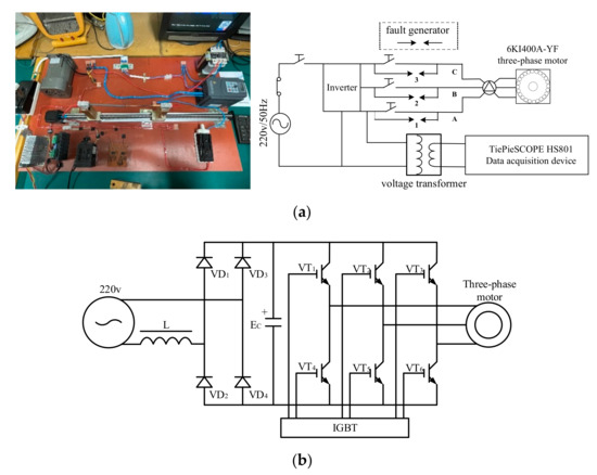
Figure 1.
Experimental platform. (a) Physical and simulation diagrams of the experimental platform; (b) Working principle diagram of inverter.
2.2. The Experiment Design
The fault arc signal is obtained by drawing—arc fault simulation. The main body of the fault occurrence device is composed of a 6 mm carbon rod and 6 mm copper rod, in which the carbon rod is used as the static electrode and the copper rod is used as the moving electrode. The electrodes are moved under the control of a stepper motor to adjust the gap between the electrodes to produce an arc. The fault occurrence device is shown in Figure 2:
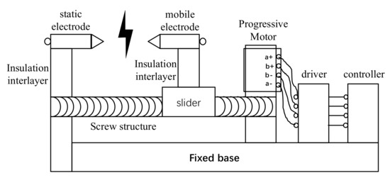
Figure 2.
Fault generator.
In order to ensure the generality of the simulation system, this paper uses the frequency converter to convert single-phase electricity into three-phase electricity, and it uses the triangle connection method to connect a 220 V three-phase motor. In this paper, when the maximum speed of the motor is working normally, one of the branches simulates the fault. The collection point is fixed in phase A, and arc faults occur in three phases of A, B and C respectively. The voltage between the collection point of phase A and the neutral line of the inverter is collected as experimental data. An experimental circuit diagram is shown in Figure 1. Four groups of experiments are carried out: namely normal, A-phase fault, B-phase fault and C-phase fault. Here, 1, 2, and 3 are the locations where faults occur. The switch is on to simulate the occurrence of faults, and the switch is closed to simulate the normal situation of branches. In total, 2000 groups of experimental data were collected for each group.
2.3. Data Acquisition and Preprocessing
The voltage frequency of the input three-phase motor is 50 kHz, the sampling number is 10,000 as the sampling condition, and the sample duration is 0.2 s, including 10 cycles of voltage waveform. When there are 15 or more fault arc features in the sample, the sample is identified as a fault sample, and a label is added at the end of the data according to its fault type. The host used in this experiment is configured with an Intel (R) Core (TM) i7-7700 hq processor, the GPU is an NVIDIA GeForce GTX 1080 Ti dual graphics card, and it has 16.00 GB running memory. Under the Windows 10 system, Python is used to realize the algorithm of the experimental system. Two thousand sets of data were collected for each group of experiments, and the training and testing datasets were allocated by 7:3.
2.4. Waveform Analysis
The waveform obtained from the three-phase fault arc simulation experiment is shown in Figure 3. Here, the abscissa is the time axis, and the unit is second (s). The ordinate is voltage, expressed in volts (V). According to the experimental waveform, the frequency converter uses SPWM, that is, sinusoidal pulse width modulation, for single-phase to three-phase conversion and speed regulation. Different from the regular high-frequency waveform with large amplitude variation, the fault is characterized by a chaotic high-frequency burr waveform with small amplitude variation. Among them, the fault characteristics of phase A are more obvious in each stage. The fault characteristics of B and C two-phase faults are different in different stages. The phase B fault is more obvious in the first and third stages, and the phase C fault is more obvious in the second and fourth stages, indicating that the phase characteristics of different faults have strong timing.
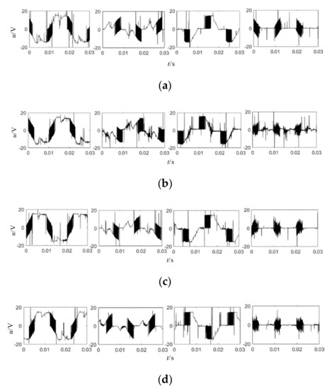
Figure 3.
Experimental waveform. (a) Normal operating state; (b) Phase A fault status; (c) Phase B fault status; (d) Phase C fault status.
Taking the A-phase fault as an example, as shown in Figure 4, due to the change of experimental environment, the different intensity of arc combustion, the uncontrollable length of arc pulling gap and the change of contact area between fault poles caused by dust after carbon rod combustion, the fault characteristics of the same type of data are quite different. Therefore, the robustness of the model is required.
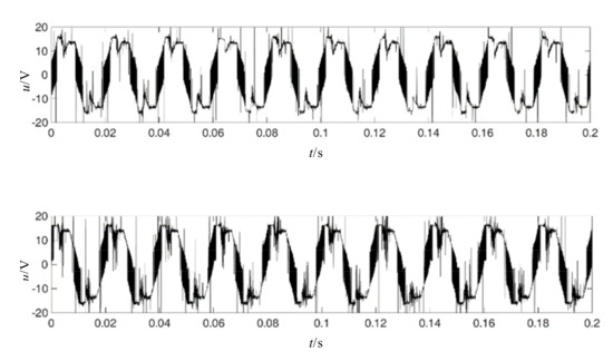
Figure 4.
A phase fault comparison chart.
3. Variational Mode Decomposition
Variational mode decomposition (VMD) [24] is an adaptive signal processing method based on the use of non-recursive and variational mode decomposition. Variational theory is derived from mathematical functional analysis. This method can suppress the aliasing of EMD by controlling the bandwidth. VMD decomposition uses an iterative search for the optimal solution of the variational model to determine the component center frequency and bandwidth of each decomposition, which is a completely non-recursive model. Its mode is defined as the AM/FM signal, and its function is expressed as:
where is the signal phase and is the instantaneous amplitude. k is the BIMF component with specific sparsity, and the optimal solution of each component is obtained by constantly updating each mode function and center frequency through iteration. For the signal, its constrained variational model is:
where represents each BIMF component composition and then represents the center frequency of each component. is the pulse signal, * is the symbol of convolution operation, and is the convolution operation.
As shown in Equations (3) and (4), in order to obtain the optimal solution of Equation (2), the initial , , values are given, and the penalty factor and Lagrange operator are introduced to update each mode and its center frequency. The specific solution steps are as follows:
After the NTH cycle, the Lagrange operator is updated according to Equation (5)
As shown in Equation (5), cyclic iteration steps (2) and (3) are carried out until the total deviation is less than the ε preset error, and the cycle is stopped to obtain the k group of modal functions.
Taking the normal state and phase A fault stage 1 as an example, the optimal solution of VMD decomposition k is 6, so the original signal f is decomposed to obtain six groups of components, and the eigenmode functions of six groups of BIMF components are obtained, as shown in Figure 5.
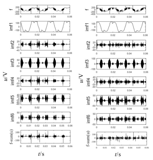
Figure 5.
Eigenmode functions of normal and faulty BIMF components.
It can be seen from the figure that there are great differences in the fault feature content among waveforms with different center frequencies, and the content of the fault feature in IMF1–IMF3 is low and similar to that in non-fault waveforms. The fault features in IMF4–IMF6 are obvious but have strong correlation with the time sequence of non-fault waveform, so it is difficult to extract.
4. GTCN Neural Network Model
4.1. GTCN Neural Network
Aiming at the difficulty of extracting the fault features of different stages and frequencies of experimental data, a GTCN neural network model is proposed in this paper. As shown in Figure 6, global temporal convolutional neural network (GTCN) consists of data preprocessing, an initial extraction layer, a feedforward network layer and a classification and recognition layer.
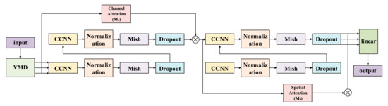
Figure 6.
GTCN neural network model.
Firstly, the signal data collected by the arc data acquisition platform are formatted, classified and sorted by the data preprocessing layer, and labels are added according to the data types. Secondly, the preprocessed data are decomposed by VMD with the optimal solution k = 6, and the decomposed IMF4, IMF5 and IMF6 are, respectively, used as the input of the three channels of the sequential convolution feedforward neural network in the GTCN network. CCNN is a causal convolutional layer, and the main body of the network is a temporal convolutional network with four layers of CCNN. The channel attention in GAM is used between the data input terminal and the second causal convolution layer, and the feedforward operation is continued after each channel is dotted with the channel attention map. The spatial attention map of each channel between the output of the second layer and the output of the fourth layer is formed after dimension reduction by point multiplication. Finally, the fused feature vectors are brought into the fully connected layer for classification and recognition. In order to improve the effect of fault classification, the Mish activation function is used as the activation function in GTCN, the Adam algorithm is used as the optimizer, and the cross-entropy function is used as the loss function. To prevent the problem of overfitting in the training process of the network, the dropout training mechanism is added into the model, and its value is set to 0.2. The main network of this model is a four-layer TCN, and the number of hidden layers is 2. The initial learning rate is 0.001. The maximum number of iterations follows.
4.2. Global Attention Mechanism
As shown in Figure 7, the Global Attention Mechanism (GAM) [25] is compared with the original CBAM Attention Mechanism; it reduces the loss of information in transmission and expands the attention span. Its working principle is shown in the GAM module. The operation is as follows:
where Mc and Ms are the attention map of channel and space, respectively, and is the dot product operation. In order to adapt the experimental data, the two-dimensional convolution in the structure is changed to one-dimensional convolution, and the original dimensional transformation of the three-dimensional data is omitted.
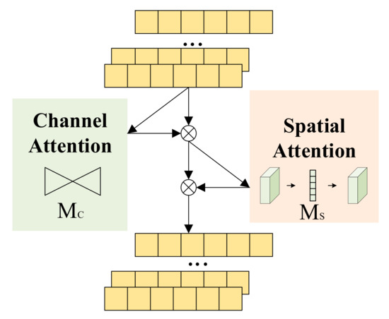
Figure 7.
Global attention mechanism.
There is a two-layer MLP in channel attention, which enhances the dependence of classification on temporal information. The spatial attention is a two-layer one-dimensional convolution, which integrates the spatial information, uses the reduction rate R and eliminates the pooling layer, so as to maximize the retention of fault and phase features.
4.3. Activation Function Selection
The function of activation function is to bring nonlinear elements into the linear model to complete nonlinear tasks such as classification. Choosing an appropriate activation function can improve the efficiency and accuracy of this kind of work. The original Temporal Convolutional Network uses the classical Relu activation function, whose function expression is shown in (9), and the function image is shown in Figure 8.

Figure 8.
Relu, PRelu and Mish activation functions.
The Relu function is not activated when the input is negative, which indicates that Relu will be invalid if the input is negative. In the back propagation process, the gradient is zero. However, the fault arc data will have negative values in the propagation process, so it is necessary to select the activation function used in the model.
The PRelu (Parametric Reasonable Linear Unit) activation function [26], that is, the activation function expressed in Equation (10) can provide a reasonable solution to the problem of Relu failure, as shown in Figure 8.
As a self-learnable activation function, its learning rate update method adopts a momentum method, namely:
Although PRelu solves the failure problem of Relu, its function curve is not smooth enough, which will lead to the lack of generalization ability when performing nonlinear work. Compared with PRelu, the Mish activation function based on the self-gating characteristic of Swish activation function is more likely to match or improve the performance of neural network architecture [27]. Its expression is as follows:
According to Equation (12) and Figure 8, the Mish activation function is a continuous, smooth, regularized and non-monotonic activation function, which performs well on gradient flows. The formula structure of multiplying the nonmodulated input with the output of the input nonlinear function eliminates the prerequisite for problems such as Relu failure.
4.4. Basic Principles of TCN
The causal convolution operation in Temporal Convolutional Network (TCN) has a logic similar to Markov chain, that is, the current input only depends on the current value and the value at the previous time, which not only ensures the timing of feature extraction but also avoids the problem of redundant network structure in order to retain temporal information. As shown in Figure 9, on the basis of causal convolution, dilated convolution does not increase the convolution kernel size and the number of network layers, but it only increases a dilated rate D, namely the time range of input data, to enhance its receptive field. The expression of extended causal convolution is:
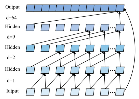
Figure 9.
Dilated Causal Convolution.
On the premise of ensuring the performance of neural networks, higher requirements are also put forward for the stability of multilayer expansive causal convolution. Residual network ResNets provide a solution for multilayer network optimization. As shown in Figure 10, in the residual block, four layers of extended causal convolution and nonlinear mapping are used to ensure the classification performance. In order to reduce the computational burden of the network model and reduce the model size, the convolution kernel size of the expanded causal convolution is 13, and the expansion rate D is 1, 2, 9 and 64, respectively. That is, the nonlinear growth method is adopted. Mish activation function and weight normalization are used between layers to improve the convergence efficiency of the network.
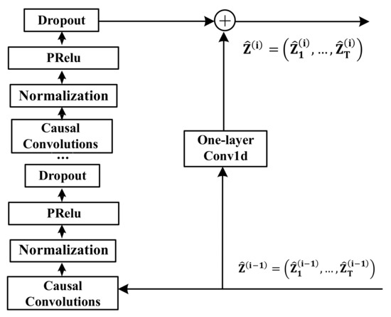
Figure 10.
TCN neural network.
5. Experiment and Result Analysis
5.1. Criteria
In this paper, accuracy rate, precision rate, recall rate, F1 value and confusion matrix are used as the evaluation criteria of the model:
In Equations (14)–(17), TP stands for the number of actual categories predicted as true categories, TN stands for the number of actual wrong categories predicted as false categories, FP stands for the number of actual wrong categories predicted as true categories, and FN stands for the number of actual right categories predicted as false categories.
5.2. The Experimental Results
Various existing models and comparative experimental designs are shown in Table 1. All kinds of existing models directly use the original data for three-phase fault detection. Each phase fault detection dataset and three-phase fault mixture dataset were used as the input of different network models for fault diagnosis and fault phase selection. Since there is no global attention in GRU, LSTM and original TCN, IMF4, IMF5 and IMF6 after VMD decomposition are superimposed and reconstructed as the input of the three networks. The Mish activation function was used in both networks. The detection results of each phase fault and fault phase selection of GTCN are compared with the detection results of traditional recurrent neural network GRU, LSTM and original TCN. The experimental results are selected after the network iteration process is stable.

Table 1.
Fault identification and phase selection accuracy of each model.
Experimental results show that the detection accuracy of GTCN is higher than that of existing deep learning fault detection models. In recurrent neural networks, the detection accuracy of the model using VMD for initial feature extraction is significantly higher than that of the model without VMD. Only models using VMD are analyzed below.
The phase selection accuracy of GRU and LSTM reached 93.87% and 96.13%, respectively. Compared with LSTM, the accuracy of fault arc detection in each phase of GRU is reduced by about 1%, and the accuracy of fault phase selection is reduced by about 2.3%. This indicates that although GRU has fewer parameters and a relatively simple structure, compared with the special gate structure of LSTM, GRU has insufficient ability to capture depth features.
The phase selection accuracy of the original TCN network is 95.37%, and the fault detection accuracy of phase A, phase B and phase C is 96.38%, 94.98% and 96.98%. Compared with the recurrent neural network, although TCN has a larger receptive field, the causal convolutional neural network loses some fault and dissimilarity features during the convolutional operation, resulting in its accuracy being similar to that of LSTM and unstable.
The fault arc phase selection accuracy of GTCN is 98.62%, and the fault detection accuracy of each phase is about 99%. Compared with the original TCN network, the classification and detection accuracy is improved by about 3%. The global attention mechanism improves the ability of the network to mine deep information by extracting faults and different features. Compared with LSTM, the fault phase selection accuracy of GTCN is increased by about 3%, indicating that GTCN has a large receptive field to sense the phase differentiation characteristics of strong timing.
To visually demonstrate the detection effect of the GTCN model, the detection results are visualized and the confusion matrix is generated, as shown in Figure 11. The larger the value on the diagonal of the confusion matrix, the better the detection effect of the model. Here, 0, 1, 2 and 3 represent the normal working state, A-phase fault state, B-phase fault state and C-phase fault state, respectively.
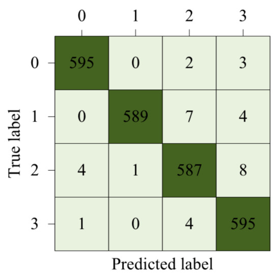
Figure 11.
Confusion matrix of GTCN three-phase fault arc detection.
In order to verify the impact of the difference of activation functions on the overall architecture, GTCN neural network models under different activation functions were trained, and the evaluation criteria were accuracy, precision, recall and F1 value.
The experimental results are shown in Table 2. The accuracy rate and recall rate of the original Relu activation function for fault phase selection reach the lowest 95%. The accuracy, precision and recall of the PRelu activation function and F1 value reached 97.75%, 97.76%, 97.75% and 97.74%, respectively. The Mish activation function in GTCN shows that the accuracy, precision, and recall of fault arc phase selection are 98.63%, while the F1 value drops slightly to 98.26%.
Table 2.
Fault phase selection accuracy of GTCN under each activation function.
The experimental results show that GTCN will appear negative during the propagation process, so the failure of Relu function reduces the accuracy of phase selection classification. In the process of GTCN iteration, the Mish activation function can better capture category features than PRelu activation function in the feature classification task. Therefore, the Mish activation function is used in GTCN for low-voltage three-phase fault arc phase selection.
6. Conclusions
In this paper, a detection method based on a global temporal convolutional network (GTCN) is proposed to solve the problem of three-phase series fault detection in a low-voltage three-phase system. The global attention mechanism and Mish activation function are used to optimize the algorithm. The simulated three-phase fault arc experiment was carried out, and VMD was used to analyze the data in the time-frequency domain and extract the initial features. The global attention mechanism improves the mining ability of deep feature information and improves the accuracy of complex fault identification.
The fault arc phase selection accuracy of the GTCN model reaches 98.62%, and the fault detection accuracy reaches 99.39%. Compared with the traditional neural network model, the GTCN model has better performance in extracting deep features and processing long time-series information, has good performance, and has a good application prospect.
However, due to the complex operation of the actual low-voltage three-phase power system, the experiment in this paper only simulates one of the typical operation states. In the future, we will continue to discuss different practical application scenarios, establish a more complete experimental database, and combine time-frequency domain analysis with spatial domain analysis to optimize low-voltage three-phase fault arc detection and phase selection models.
Author Contributions
Conceptualization, Q.Y.; Data curation, L.Z.; Project administration, Q.Y.; Resources, Q.Y.; Software, L.Z.; Supervision, Y.Y.; Validation, Y.Y.; Writing—original draft, L.Z. All authors have read and agreed to the published version of the manuscript.
Funding
This work was supported by [2018 China Postdoctoral Science Foundation] grant number [No. 2018M641287] and [The National Natural Science Foundation of China] grant number [No. 61601172].
Conflicts of Interest
The authors declare no conflict of interest.
References
- Wang, Y.; Liu, L.M.; Li, S.N.; Feng, L.; Liu, Q.L.; Song, R.N. Fault Arc Detection Based on Empirical Wavelet Transform Composite entropy value and feature fusion. Power Grid Technol. 2022, 2022, 1–8. [Google Scholar]
- Chen, X.; Leng, J.W.; Li, H.F. Series fault arc identification method based on all-phase spectrum and deep learning. Prot. Control Electr. Power Syst. 2020, 48, 1–8. [Google Scholar]
- Zhang, T.; Wang, H.Q.; Zhang, Z.C.; Yang, K. Arc fault detection method based on self-normalized neural network. Chin. J. Sci. Instrum. 2021, 42, 141–149. [Google Scholar] [CrossRef]
- Zhang, T.; Zhang, R.; Wang, H.; Tu, R.; Yang, K. Series AC Arc Fault Diagnosis Based on Data Enhancement and Adaptive Asymmetric Convolutional Neural Network. IEEE Sens. J. 2021, 21, 20665–20673. [Google Scholar] [CrossRef]
- Su, J.J.; Xu, Z.H. Research on fault arc diagnosis method based on chaotic fractal theory. Electr. Mach. Control 2021, 25, 125–133. [Google Scholar]
- Hu, C.Q.; Qu, N.; Zhang, S. Series arc fault detection based on continuous wavelet transform and DRSN-CW with limited source data. Sci. Rep. 2022, 12, 12809. [Google Scholar] [CrossRef]
- Guo, F.Y.; Gao, H.X.; Wang, Z.Y.; Ren, Z.L.; Li, X.J. Characteristics analysis of series fault arc based on SVD filter. J. Electr. Power Syst. Autom. 2019, 31, 39–44. [Google Scholar]
- Wang, Z.L.; Gao, H.X.; Guo, F.Y. Application of SVD in series fault arc detection and phase selection. China Saf. Prod. Sci. Technol. 2020, 16, 160–165. [Google Scholar]
- Niu, Z.Y.; Zhong, G.Q.; Yu, H. A review on the attention mechanism of deep learning. Neurocomputing 2021, 452, 48–62. [Google Scholar] [CrossRef]
- Chen, Z.H.; Wu, M.; Zhao, R.; Guretno, F.; Yan, R.Q.; Li, X.L. Machine Remaining Useful Life Prediction via an Attention-Based Deep Learning Approach. IEEE Trans. Ind. Electron. 2021, 68, 2521–2531. [Google Scholar] [CrossRef]
- Kruthiventi, S.S.S.; Ayush, K.; Babu, R.V. DeepFix: A Fully Convolutional Neural Network for Predicting Human Eye Fixations. IEEE Trans. Image Process. 2017, 26, 4446–4456. [Google Scholar] [CrossRef] [PubMed]
- Yan, C.; Hao, Y.; Li, L.; Yin, J.; Liu, A.; Mao, Z.; Chen, Z.; Gao, X. Task-Adaptive Attention for Image Captioning. IEEE Trans. Circuits Syst. Video Technol. 2022, 32, 43–51. [Google Scholar] [CrossRef]
- Chen, Y.; Liu, L.; Phonevilay, V.; Gu, K.; Xia, R.; Xie, J.; Zhang, Q.; Yang, K. Image super-resolution reconstruction based on feature map attention mechanism. Appl. Intell. 2021, 51, 4367–4380. [Google Scholar] [CrossRef]
- Liu, F.; Pu, Z.H.; Zhang, S.C. Unmanned aerial vehicle (uav) multiple target tracking algorithm based on attention features fusion. Control. Decis. 2021, 2021, 1–9. [Google Scholar]
- Wang, H.; Liu, Z.L.; Peng, D.D.; Qin, Y. Understanding and Learning Discriminant Features based on Multiattention 1DCNN for Wheelset Bearing Fault Diagnosis. IEEE Trans. Ind. Inform. 2020, 16, 5735–5745. [Google Scholar] [CrossRef]
- Feng, Y.; Chen, J.L.; Zhang, T.C.; He, S.L.; Xu, E.Y.; Zhou, Z.T. Semi-supervised meta-learning networks with squeeze-and-excitation attention for few-shot fault diagnosis. ISA Trans. 2022, 120, 383–401. [Google Scholar] [CrossRef]
- Cap, Q.H.; Uga, H.; Kagiwada, S.; Iyatomi, H. LeafGAN: An Effective Data Augmentation Method for Practical Plant Disease Diagnosis. IEEE Trans. Autom. Sci. Eng. 2022, 19, 1258–1267. [Google Scholar] [CrossRef]
- Bai, S.; Kolter, J.Z.; Koltun, V. An empirical evaluation of generic convolutional and recurrent networks for sequence modeling. arXiv 2018, arXiv:1803.01271. [Google Scholar]
- Yu, F.; Koltun, V. Multi-scale context aggregation by dilated convolutions. In Proceedings of the International Conference on Learning Representations, New Orleans, LA, USA, 6–9 May 2019. [Google Scholar]
- He, K.M.; Zhang, X.Y.; Ren, S.Q.; Sun, J. Deep residual learning for image recognition. In Proceedings of the IEEE Conference on Computer Vision and Pattern Recognition, Las Vegas, NV, USA, 27–30 June 2016; IEEE Press: Washington, DC, USA, 2016; pp. 770–778. [Google Scholar]
- Xu, Y.Q.; Xu, G.X.; Ma, C.; An, Z.L. An Advancing Temporal Convolutional Network for 5G Latency Services via Automatic Modulation Recognition. IEEE Trans. Circuits Syst. II-Express Briefs 2022, 69, 3002–3006. [Google Scholar] [CrossRef]
- Lin, J.; van Wijngaarden, A.J.D.; Wang, K.C.; Smith, M.C. Speech Enhancement Using Multi-Stage Self-Attentive Temporal Convolutional Networks. IEEE-ACM Trans. Audio Speech Lang. Process. 2021, 29, 3440–3450. [Google Scholar] [CrossRef]
- Bian, H.H.; Wang, Q.; Xu, G.Z.; Zhao, X. Load forecasting of hybrid deep learning model considering accumulated temperature effect. Energy Rep. 2022, 8, 205–215. [Google Scholar] [CrossRef]
- Dominique, Z.; Konstantin, D. Variational Mode Decomposition. IEEE Trans. Signal Process. A Publ. IEEE Signal Process. Soc. 2014, 62, 531–544. [Google Scholar]
- Yichao, L.; Zongru, S.; Nico, H. Global Attention Mechanism: Retain Information to Enhance Channel-Spatial Interactions. arXiv 2021, arXiv:2112.0556. [Google Scholar]
- He, K.M.; Zhang, X.Y.; Ren, S.Q. Delving deep into rectifiers: Surpassing human-level performance on image net classification. In Proceedings of the IEEE International Conference on Computer Vision, Santiago, Chile, 7–13 December 2015; IEEE Press: Washington, DC, USA, 2015; pp. 1026–1034. [Google Scholar]
- Mish, M.D. A self regularized non-monotonic neuralacti-vation function. arXiv 2020, arXiv:1908.08681. [Google Scholar]


Publisher’s Note: MDPI stays neutral with regard to jurisdictional claims in published maps and institutional affiliations. |
© 2022 by the authors. Licensee MDPI, Basel, Switzerland. This article is an open access article distributed under the terms and conditions of the Creative Commons Attribution (CC BY) license (https://creativecommons.org/licenses/by/4.0/).