Finite Element Simulation of HELICOIL^® Inserts

Abstract

This paper details the possibility of simulating HELICOIL^® inserts using Finite Element Analysis and contact technology. The main procedure is based on the use of contact elements in the Glue–Cohesive setting, which is usually considered for the simulation of composites. The contact represents the behaviour of an interface, including the HELICOIL^® insert, the sample threads, and the screw threads. The behaviour of the cohesive contact is determined by a multi-linear curve, and is described by several parameters. Our main goal is to determine the number of parameters and their values to provide a defined accuracy. The sample is made of ABS-M30 material, while the screw is made of steel. The Finite Element Model Updating method is used to determine the parameters from experimental data. The problem regarding the addition of a point (parameter) to a multi-linear curve is solved using the principle of halving intervals. A gradient approach combined with a penalisation method is used to identify the parameters of the interface model. The simulation results are compared with data obtained through Digital Image Correlation measurements.

1. Introduction

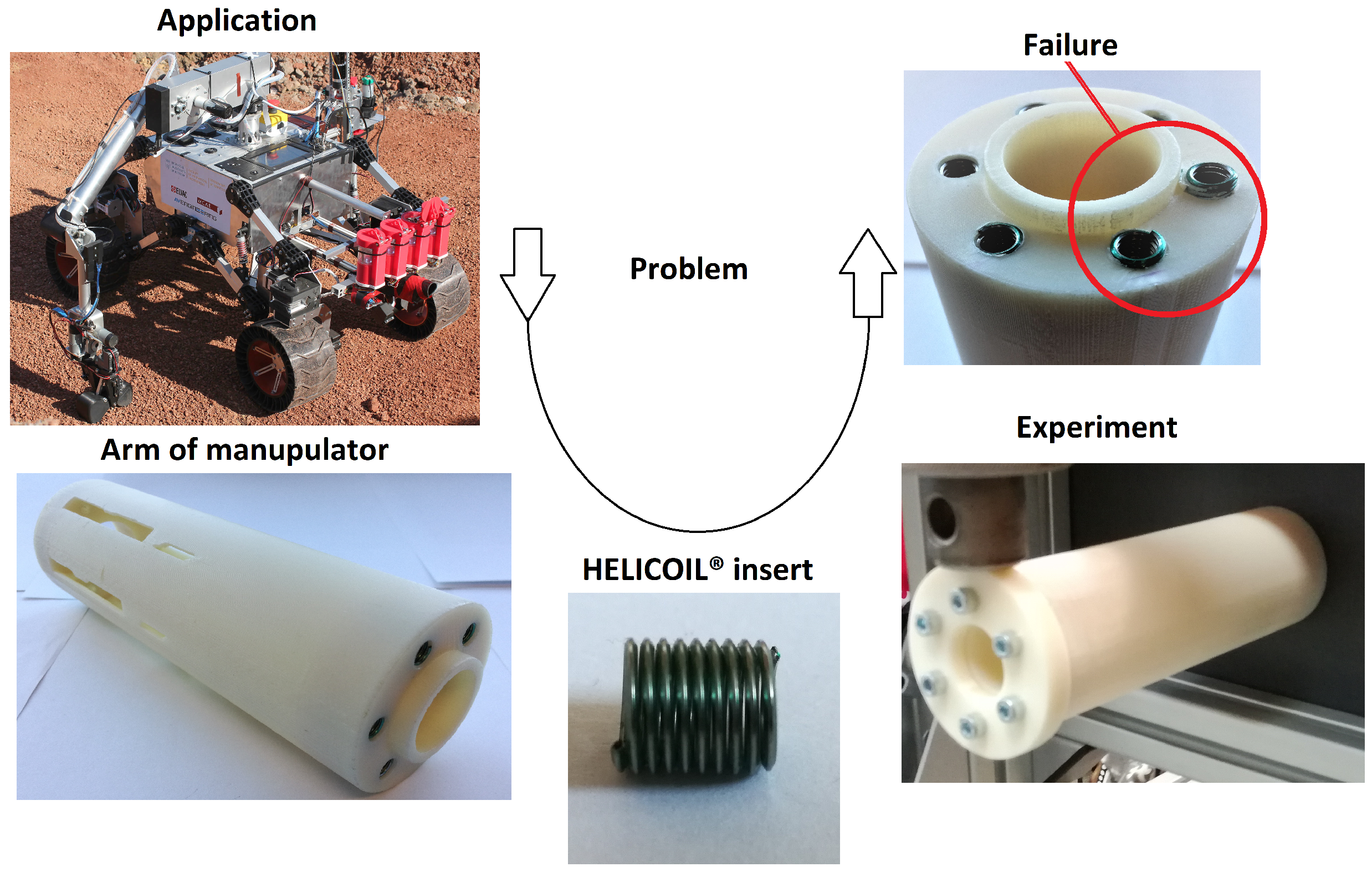
HELICOIL^® inserts are a type of threaded insert, which are typically used to repair damaged threads or to increase the load-bearing capacity of a bolt connection for softer materials. The insert allows for a better stress distribution in the threads and, thus, an increase in the load-bearing capacity of the connection [1]. This system is suitable for connections which are often disassembled, and where the thread may be damaged by wear. The application range of threaded inserts is wide; however, in our case it is used in robotics, for the design of manipulator arms [2] (see Figure 1).

Experiments and simulations with HELICOIL^® inserts have been described in a relatively small number of articles. In [2], tension experiments with different force–time dependences have been presented and, for the simulation Finite Element Analysis (FEA), the MSC Marc software [3] was used. HELICOIL^® inserts are simulated using a so-called cohesive zone, interpreted as a part of the body that contains the threads and the threaded insert. The cohesive zone is modelled as a type of contact. In [4], experiments based on compression and torsion tests have been published. In addition to experiments (e.g., tightening tests, crash load tests, strength tests), the use of Finite Element Analysis (FEA; Abaqus, simplified with axisymmetry) has been presented in [5]. Another procedure to reduce the computational complexity has been presented in [6]. FEA is used for the simulation of one thread and, for the simulation, the entire screw connection is applied as an interface to simplify the thread hypotheses.

The cohesive zone model was developed to simulate damage in composite laminates [7]. At present, this model can be used in various software (FEA), as a type of element. So-called interface elements are available, for example, in MSC Marc [3] and ANSYS [8]. These elements connect two different bodies; in this case, a specimen and a screw. Simplistically, we can imagine that a spring (normal and shear orientation) is defined between two elements (one for the specimen and one for the screw). The stiffness varies depending on the relative position of the two elements. The behaviour of the spring is non-linear and is defined by an equation. The software implementation may vary. The behaviour of the interface (cohesive zone) can be represented by a bilinear constitutive equation [3,8], an exponential model, or a linear–exponential model. However, while models have been developed for the delamination of composite laminates [9], no similar theoretical model has been published for HELICOIL^® inserts. Contact elements [3] allow us to define the behaviour of the cohesion zone using a multi-linear curve. We assume that a multi-linear curve can be described by a set of parameters. The interface model parameters in [2] were determined by hand, and the paper did not include a more detailed analysis.

In this paper, we use the Finite Element Model Updating (FEMU) approach to identify the interface model parameters. In particular, the Finite Element Model Updating (FEMU) approach is used to identify material parameters through a FEA simulation; see [10]. This approach has been used in several areas; see, for example, [11] (indentation test) and [12] (composite materials). For the identification of parameters in an interface model, the extended Kalman filter (EKF) has been used in [13].

Experiments and simulations of the behaviour of screws (with threads) can be found more frequently in the literature. Experiments using elevated strain rates with results have been presented in [14], and experiments with 2D simulations have been presented in [15]. 3D thread simulations have been presented in [16,17]; for shear behaviour, see [18]. Screws are also used in biomechanical areas; see [19]. The measured (Force–Displacement) curves in this case were very similar to those of HELICOIL^® inserts; see, for example, [2,15]. The curve gradually changes until the thread breaks, there are no jumps in this first part, and the experiments correspond very well to the simulations. In the second part of the curve, both the simulation and the various experiments differ more significantly, and contain significant jumps (i.e., the so-called saw curve appears). In this part, there seems to have already been significant breaks, which significantly affects the results.

In the paper we used the material ABS-M30, which presents a time-dependent behaviour, see [20]. This behaviour can be expected even with a threaded insert applied to the material [2]. Currently used cohesive zone models [3], represented in terms of stress–displacement dependence, cannot capture time-dependent behaviour. Neither a time-dependent nor a time-independent model was found for HELICOIL^® inserts. The break occurs in the area of the thread; see [2,15]. Here, we simulate this area using the cohesion zone. Therefore, we only consider the linearly elastic behaviour of the specimen material.

In this article, we use penalty functions to dampen or suppress unwanted behaviours. Penalty methods are generally used in constrained optimisation; see, for example, [21,22], or [23]. This method has been used in many areas; see [24] or [25]. For example, the volume penalisation method has been used to solve model obstacles in viscous flows; see [26]. A basic idea of the approach applied to model fluid–porous–solid systems is to penalise solid obstacles as a porous medium whose permeability g tends to zero.

The Digital Image Correlation method (DIC) [27] optically measures macroscopic parameters, such as displacement. A contrast pattern is applied to the surface of the sample. Consider a test specimen that is illuminated by a light source. Its deformation corresponds to the difference between the light reflected by an undeformed object and that by the deformed object. This method is independent of other experimental equipment, and was used to validate the results [28].

2. Background

In [2], the HELICOIL^® insert was replaced by a contact with a cohesive zone setting for simulation purposes. The cohesive zone behaviour was defined by a multi-linear curve, which was identified manually. The follow-up step was to identify this curve using a gradient algorithm. During testing, it was found that the task occasionally converges to a sawtooth waveform (see Appendix A) in the initial part of the curve. This problem could be corrected manually; however, this is inappropriate for practical use. The second option was to find or design a suitable algorithm that would not lead to a sawtooth waveform. The last option was to design a mathematical model of the HELICOIL^® insert that would clearly prescribe the shape, such that the problem would not occur. From our point of view, the second option was the most logical; that is, to test other known algorithms. During testing, it was found that the sawtooth waveform arises depending on:

• The number and position of the points of the multi-linear curve;
• The settings of the algorithm used;
• The magnitude of the multi-linear curve update.

Conditions were set that limited the formation of the saw curve shape. These conditions relate to the method of identifying the multi-linear curve, not the definition of the curve. The curve definition—that is, the mathematical model of the HELICOIL^® insert—will be the next step, and multi-linear curves can be used for its analysis and validation. The associated conditions are as follows:

• Gradual adding of points to the curve;
• Frequent updating of the gradient after a pre-defined number of cycles;
• Multi-linear curve update size limit;
• Reducing the effect of thread damage at the end of the measured time, when the HELICOIL^® insert is gradually pulled out of the hole and the threads are already broken.

The first point led to a proposal inspired by the interval halving method, which adds only one point to the interval found in the previous cycle. Next, we defined a partial objective function, which describes the influence of each point of the multi-linear curve on the value of the objective function, as well as a screening approach, which identifies the most appropriate place to add a new point. Thus, the curve could be identified successively with an increasing number of points, until the defined accuracy given by the objective function value is met. The points identified in previous cycles no longer change, in some cases, so a simple constraint based on the sign of the gradient was added to reduce the number of points identified.

The second point added to the convergence check, allowing for checking of the maximum number of cycles per gradient calculation. The third point led to the use of a so-called normalised gradient, for which the magnitude of the added value can be controlled very well. The last point led to the correction of the values of the objective function with respect to time.

These modifications were implemented into the algorithm and objective function using a penalty function. In the resulting algorithm, the formation of a sawtooth waveform no longer occurred in the test example. The conditions were not applied to the multi-linear curve; which, in our opinion, would lead to the construction of a mathematical model for the HELICOIL^® insert. Instead, the conditions were applied to the method of identifying the parameters of the multi-linear curve. The proposed identification method differs from standard procedures and, in our opinion, some of the modifications used may be useful in other cases.

3. Task Definition

In [2], for FEA, it was proposed to replace the HELICOIL^® insert with a type of cohesive contact, where the behaviour of the cohesive contact was defined by a multi-linear curve, which was determined by trial and error. This method is not suitable for practical use, and does not guarantee optimal results.

The main objective of the paper is to present an algorithm designed to solve the given problem, to highlight its application, and to test the results of the solution using the DIC method.

The following simplification conditions are considered in the article:

• We assume a correlation between the measured data (Force–Displacement) and a multi-linear curve (Shear Stress–Displacement) which defines cohesive zone;
• The behaviour of all materials is considered to be linearly elastic;
• The initial estimate is based on the bilinear model of a cohesive zone;
• The interface (cohesive contact) is defined by the normal stress–displacement curve and the shear stress–displacement curve;
• The influence of normal stress–displacement is assumed to be negligible. It is constant and the same for all analyses performed;
• Time-independent behaviour is assumed;
• The behaviour is sufficiently described by a simple tensile test. Only one experiment is used as input to the identification process;
• The threads (comprising a screw and a hole) are not modelled.

The proposed algorithm is described in Section 4. The application itself is split into three sections: the first describes the experiment (Section 5), the second describes the simulation model (Section 6), and the third describes the identification process and results (Section 7). Finally, a comparison of the results with the data obtained with DIC is presented in Section 8.

4. Materials and Methods

In this paper, we use following notation: ${\mathbb{N}}^{+}$ is the set of positive whole numbers and $\mathbb{R}$ is the set of all real numbers.

Suppose a relation $\mathsf{\Gamma }$ is a FEM simulation, which maps inputs $\mathbf{P}$ and $\mathbf{R}$ to an output $\mathbf{Y}$, as follows:

$$\mathbf{Y}=\mathsf{\Gamma }(\mathbf{P},\mathbf{R}),$$

(1)

where

• $\mathbf{P}=\{[u_i,p_i]:i=0,1,\dots ,N\}$ is a set of points of a multi-linear curve (parameter points), and $N+1$ is the number of points ($2\le N\in {\mathbb{N}}^{+}$). Each point is defined by the position $u_i\in \mathbb{R}$ and by the parameter value $p_i\in \mathbb{R}$. The parameter value $p_i$ is variable, the position $u_i$ is a constant and, for two positions, the following are satisfied: $u_i<u_{i+1}:i=0,1,\dots ,N-1$, and $[u_i,p_i],[u_{i+1},p_{i+1}]\in \mathbf{P}$. For simplicity, we consider a vector of parameters $p=[p_i:i=0,1,\dots ,N]$. We assume that the initial estimate is for $N=2$, and N is also variable;
• $\mathbf{R}=[[t_k,r_k]:k=0,1,\dots ,N_T]$, $t_k\in \mathbb{R}$, $r_k\in {\mathbb{R}}^n$, n, $N_T$ are a vector of loading steps, the time step, the loading step, the dimension of the loading, and the number of loading steps, respectively. We assume that $N\le N_T$ holds for the number of parameter points;
• $\mathbf{Y}=[[t_k,y_k]:k=0,1,\dots ,N_T]$, $y_k\in {\mathbb{R}}^m$, m are the set of results, the result step, and the dimension of the results, respectively.

Let a vector of data $\widehat{\mathbf{Y}}$ obtained from an experiment be as follows:

$$\widehat{\mathbf{Y}}=[[t_k,{\widehat{y}}_k]:k=0,1,\dots ,N_T],{\widehat{y}}_k\in {\mathbb{R}}^m,$$

(2)

where ${\widehat{y}}_k$ denote the results of experiment k.

A classical objective function (COF) $g(\mathbf{Y},\widehat{\mathbf{Y}})$ indicates the agreement of the current solution with the experiment, which is described as follows:

$$g(\mathbf{Y},\widehat{\mathbf{Y}})={\parallel \widehat{\mathbf{Y}}-\mathbf{Y}\parallel }_C,$$

(3)

where $\parallel \widehat{\mathbf{Y}}{-\mathbf{Y}\parallel }_C$ is the norm for COF calculation.

A partial objective function $f_i(\mathbf{Y},\widehat{\mathbf{Y}})$ (POF) describes the effect of the $i^{\mathrm{th}}$ parameter on the agreement of the current solution with the experiment, described as follows:

$$f_i(\mathbf{Y},\widehat{\mathbf{Y}})={\parallel \widehat{\mathbf{Y}}-\mathbf{Y}\parallel }_i,$$

(4)

where $\parallel \widehat{\mathbf{Y}}{-\mathbf{Y}\parallel }_i$ is the norm for POF calculation. An objective function, $f(\mathbf{Y},\widehat{\mathbf{Y}})$ (OF), is calculated as follows:

$$f(\mathbf{Y},\widehat{\mathbf{Y}})=\sum _{i=1}^N{f}_i(\mathbf{Y},\widehat{\mathbf{Y}}).$$

(5)

Both types of objective functions—that is, $g(\mathbf{Y},\widehat{\mathbf{Y}})$, $f(\mathbf{Y},\widehat{\mathbf{Y}})$—include the effects of all parameters, so we will assume that they are interchangeable and the following applies: $g(\mathbf{Y},\widehat{\mathbf{Y}})\approx f(\mathbf{Y},\widehat{\mathbf{Y}})$. In this article, these values are briefly referred to as g, $f_i$, and f, respectively.

This section describes the basic considerations for finding the values of the parameters that represent a multi-linear curve. The procedure is designed with regard to the occurrence of local minima for some parameters during the identification process, and can be divided into several parts. First, the idea of the solution is described in Section 4.1. Second, the objective functions are defined in Section 4.2. Third, a minimisation method is described in Section 4.3. Fourth, the screening is described in Section 4.4. Finally, two algorithms are presented in Section 4.5: a basic framework for the whole algorithm and a minimisation algorithm based on the minimisation method.

4.1. Idea of Solution

We assumed that the identification can be described as a type of optimisation. If we want to identify the values of parameters, we have to first know their number N (and positions). The value N is variable, and we can add ($N\leftarrow N+1$) a point $[u_i,p_i]$ to the current vector of parameter points $\mathbf{P}$. Note that a similar procedure can be applied when deleting a parameter point; however, this is not considered in this article and, therefore, is not addressed here. Simply put, we solve two problems, described as follows:

• Minimisation method: Find the vector of parameter values $\mathbf{p}$ (the number of parameter points N does not change):

  $${\mathbf{P}}^{*},f^{*}\leftarrow {\mathbf{min}}_{\mathbf{p},{\epsilon }_{min}}f(\mathsf{\Gamma }(\mathbf{P},\mathbf{R}),\widehat{\mathbf{Y}}),$$

  (6)

  where ${\epsilon }_{min}$ is the minimum convergence rate, ${\mathbf{P}}^{*}$ is the set of points with the found parameter values, and $f^{*}$ is the minimum OF value found.
• Screening: Find a new set of parameter points $\mathbf{P}$ (the number of parameter points N increases). The step is represented by a screening procedure $S(\mathbf{P},\dots )$:

  $$\mathbf{P}\leftarrow S(\mathbf{P},\dots ).$$

  (7)

The convergence rate $\epsilon$ is monitored during minimisation (6). If it drops below the minimum convergence rate ${\epsilon }_{min}$, the screening procedure is started. Suppose we look for the results of the minimisation problem using an iterative approach, where a and $a+1$ represent two consecutive steps in our simulation. The current convergence rate (the difference between two consecutive steps) is defined as follows:    

$$\epsilon =\frac{f(\mathsf{\Gamma }({\mathbf{P}}^{\mathbf{a}},\mathbf{R}),\widehat{\mathbf{Y}})-f(\mathsf{\Gamma }({\mathbf{P}}^{\mathbf{a}+\mathbf{1}},\mathbf{R}),\widehat{\mathbf{Y}})}{f(\mathsf{\Gamma }({\mathbf{P}}^{\mathbf{a}},\mathbf{R}),\widehat{\mathbf{Y}})}.$$

(8)

4.2. Objective Functions

The vector of data $\widehat{\mathbf{Y}}$ and the vector of results $\mathbf{Y}$ are used as inputs to the objective functions. It is obvious that the $y_k$ values are obtained from FEA, while the ${\widehat{y}}_k$ values are obtained from an experiment. The dimension and the physical meaning of both is the same. We assume deformation loading in one axis (i.e., $n=1$) in this article. The results contain a vector $[t_k,F_k]$ ($m=1$), where $t_k$ and $F_k$ are the $k^{\mathrm{th}}$ time point [s] and the $k^{\mathrm{th}}$ force [N], respectively. The time points are the same for vectors $\mathbf{R}$, $\mathbf{Y}$, and $\widehat{\mathbf{Y}}$.

Based on the least squares method, COF $g(\mathbf{Y},\widehat{\mathbf{Y}})$ is defined by the following norm:

$$\parallel \widehat{\mathbf{Y}}{-\mathbf{Y}\parallel }_C=\frac{1}{N_T}\sum _{k=1}^{N_T}{(F_k^{\mathrm{EXP}}-F_k^{\mathrm{FEA}})}^2,\left[N^2\right],$$

(9)

where the superscript FEA denotes an element of the vector $\mathbf{Y}$ and the superscript EXP denotes an element of the vector $\widehat{\mathbf{Y}}$.

For the use of some methods, it may be advantageous to divide the OF into several parts. We want individual POFs to indicate the influence of individual parameters on the result. Therefore, there are the same number of POFs as the searched parameters. The parameter point is described by its position $u_i$ and by the value of the parameter itself $p_i$, as defined in the previous section. Suppose a POF $f_i(\mathbf{Y},\widehat{\mathbf{Y}})$ is defined in the following form:

$$\parallel \widehat{\mathbf{Y}}{-\mathbf{Y}\parallel }_i=\frac{1}{N_T}\sum _{k=1}^{N_T}{(F_k^{\mathrm{EXP}}-F_k^{\mathrm{FEA}})}^2{h}_t(t_k)h_p(t_k,\dots ),\left[N^2\right],$$

(10)

where $h_t(t_k)$ and $h_p(t_k,\dots )$ are correction functions.

We define a time correction function $h_t(t_k)$, which reduces the effect of data differences with increasing time. The time correction function is defined as follows:

$$h_t(t_k)=a_1+a_2{t}_k:0\le h_t(t_k)\le 1,[-],$$

(11)

where $a_1$ and $a_2$ are parameters of the time correction function.

A parameter correction function $h_p(t_k,p_i)$ is used to include the effect of the $i^{\mathrm{th}}$ parameter. To determine $h_p(t_k,p_i)$, we start from the classical objective function and attempt to identify the effect of the parameter, as follows:

$$\frac{\partial \parallel \widehat{\mathbf{Y}}{-\mathsf{\Gamma }(\mathbf{P},\mathbf{R})\parallel }_C}{\partial p_i}=\frac{\partial }{\partial p_i}(\frac{1}{N_T}\sum _{k=1}^{N_T}{(F_k^{\mathrm{EXP}}-F_k^{\mathrm{FEA}})}^2)=\frac{2}{N_T}\sum _{k=1}^{N_T}(F_k^{\mathrm{EXP}}-F_k^{\mathrm{FEA}})\frac{\partial \mathsf{\Gamma }(\mathbf{P},\mathbf{R})}{\partial p_i}.$$

We use the forward difference formula to solve the partial derivative, as follows:

$$\frac{\partial \mathsf{\Gamma }(\mathbf{P},\mathbf{R})}{\partial p_i}\approx \frac{\mathsf{\Gamma }(\{\dots [u_i,p_i+\Delta p],\dots \},\mathbf{R})-\mathsf{\Gamma }(\{\dots [u_i,p_i],\dots \},\mathbf{R})}{\Delta p}.$$

(12)

Here, the value $\Delta p$ is the search step size, and we use the same value for all parameters. Based on Equations (1), (9), and (12), we assume that the parameter correction function will correspond to a difference of the forces $\Delta F_{i,k}^{\mathrm{FEA}}$, as follows:

$$\Delta F_{i,k}^{\mathrm{FEA}}=F_k^{\mathrm{FEA}}-F_{i,k}^{\mathrm{FEA}},\left[N\right],$$

(13)

where k is the subscript of the time point, i is the subscript of the parameter ($p_i+\Delta p$), $F_k^{\mathrm{FEM}}$ is a reference value for the force, and $F_{i,k}^{\mathrm{FEM}}$ is a modified value for the force. The reference value is taken from the current best solution. The parameter correction function is designed as follows:

$$h_p(t_k,p_i)=\frac{\left|\Delta F_{i,k}^{\mathrm{FEM}}\right|}{\parallel \Delta F_{i,k}^{\mathrm{FEM}}{\parallel }_{\infty ,i}}:0\le h_p(t_k,p_i)\le 1,[-],$$

(14)

where $\parallel \Delta F_{i,k}^{\mathrm{FEM}}{\parallel }_{\infty ,i}$ is an infinite norm.

4.3. Minimisation Method

Many methods described in the literature can be used to solve minimisation problems (6). We first assumed that we are able to find a local/global minimum. However, in the task, we solve the problem (6) repeatedly with a different number of parameters, and assume a gradually increasing number of parameters. Some parameters may reach a local minimum earlier if parameter values are read from the previous minimisation phase. Other parameters may reach theirs later, if they were added in the previous screening phase. The solution method was designed with this problem in mind.

Our update strategy is based on the following iterative formula for a parameter value:

$$p_i^{a+1}=p_i^a+\Delta p_i^a=p_i^a+d_i^a\Delta p,$$

(15)

where $\Delta p$, $\Delta p_i^a$, and $d_i^a$ are the search step size, step size, and search direction, respectively, and a and $a+1$ again represent two consecutive steps. For simplicity, we chose the same search step size for all parameters. For two consecutive steps, we require:

$$f(\mathsf{\Gamma }({\mathbf{P}}^{\mathbf{a}+\mathbf{1}},\mathbf{R}),\widehat{\mathbf{Y}})-f(\mathsf{\Gamma }({\mathbf{P}}^{\mathbf{a}},\mathbf{R}),\widehat{\mathbf{Y}})<0.$$

(16)

From (5) and the Taylor polynomial of the first degree of a function of N variables, the following applies ($f_j(\mathsf{\Gamma }({\mathbf{P}}^{\mathbf{a}},\mathbf{R}),\widehat{\mathbf{Y}})=f_j^a$):

$$\sum _{j=1}^N(\sum _{i=1}^N\frac{\partial f_j^a}{\partial p_i}\Delta p_i^a+r_j^a)<0,$$

(17)

where $r_j^a$ is a residual value of the $j^{\mathrm{th}}$ POF. We can use the forward differences, as follows:

$$\frac{\partial f_j^a}{\partial p_i}\approx \frac{f_j(\mathsf{\Gamma }([\dots ,[u_i,p_i^a+\Delta p_i^{*}],\dots ],\mathbf{R}),\widehat{\mathbf{Y}})-f_j(\mathsf{\Gamma }([\dots ,[u_i,p_i^a],\dots ],\mathbf{R}),\widehat{\mathbf{Y}})}{\Delta p_i^{*}}=\frac{\Delta f_{j,\Delta i}^a}{\Delta p_i^{*}},$$

$$\frac{\partial f^a}{\partial p_i}\approx \frac{f(\mathsf{\Gamma }([\dots ,[u_i,p_i^a+\Delta p_i^{*}],\dots ],\mathbf{R}),\widehat{\mathbf{Y}})-f(\mathsf{\Gamma }([\dots ,[u_i,p_i^a],\dots ],\mathbf{R}),\widehat{\mathbf{Y}})}{\Delta p_i^{*}}=\frac{\Delta f_{\Delta i}^a}{\Delta p_i^{*}},$$

where $\Delta f_{j,\Delta i}^a$ is the difference for the $j^{\mathrm{th}}$ POF, $\Delta f_{\Delta i}^a$ is the difference for the OF, and $\Delta p_i^{*}$ is the parameter change. The Equation (17) changes as follows:

$$\sum _{j=1}^N(\sum _{i=1}^N\frac{\Delta f_{j,\Delta i}^a}{\Delta p_i^{*}}\Delta p_i^a+r_j^a)<0,$$

(18)

and can also be modified as follows:

$$\sum _{i=1}^N\frac{\Delta p_i^a}{\Delta p_i^{*}}(\sum _{j=1}^N\Delta f_{j,\Delta i}^s+r_i^a)=\sum _{i=1}^N\frac{\Delta p_i^a}{\Delta p_i^{*}}(\Delta f_{\Delta i}^a)<0,$$

(19)

where $r_i^a$ is a residual value of $i^{\mathrm{th}}$ parameter, and we assume that $r_i^a\approx 0$. $\Delta p_i^a$ and $\Delta p_i^{*}$ can generally have different sizes and signs. Therefore, we introduce the following condition:

$$sig(\Delta p_i^a)=sig(\Delta p_i^{*}).$$

(20)

The condition (20) must be fulfilled, which ensures that a sign vector is obtained. The initial values of the sign vector are:

$$K^0=[{\kappa }_i^0=1:i=1,2,\dots ,N].$$

(21)

The elements of the sign vector are calculated as follows:

$${\kappa }_i^{a+1}=\mathbf{IF}\Delta f_{\Delta i}^a>-r_{min}\approx 0\left\{\begin{array}{c}\hfill \mathbf{THEN}-{\kappa }_i^a,\hfill \\ \hfill \mathbf{ELSE}{\kappa }_i^a,\hfill \end{array}\right.$$

(22)

where $r_{min}$ is a residual value.

A penalisation function ${\varphi }_i^a$ for the search direction (15) is defined as follows:

$${\varphi }_i^a=\mathbf{IF}(\Delta f_{\Delta i}^a>0)\left\{\begin{array}{c}\hfill \mathbf{THEN}0,\hfill \\ \hfill \mathbf{ELSE}1.\hfill \end{array}\right.$$

(23)

For all parameters, we define ${\Phi }^s=[{\varphi }_i^s:i=1,2,\dots ,N]$ as a penalty vector. Note that, if we introduce the sign vector $K^a$ in the form ${\kappa }_i^a\in \{1,0,-1\}$ (as in (23)), then ${\varphi }_i^a=\left|{\kappa }_i^a\right|$ is valid.

To estimate the value of the parameter in the next step $p_i^{a+1}$, it is sufficient to determine the value of the search direction $d_i^a$ in the interval $0\le d_i^a\le 1$. For the value $d_i^a=0$, the value of the parameter does not change ($p_i^{a+1}=p_i^a$); meanwhile, for the value $d_i^a=1$, the value of the parameter changes by $\Delta p$, as follows: $p_i^{a+1}=p_i^a+\Delta p$. The search direction is determined as follows:

$$d_i^a=\mathbf{IF}{\parallel {\varphi }_i^a\Delta f_{\Delta i}^a\parallel }_{\infty ,i}\ne 0\left\{\begin{array}{c}\hfill \mathbf{THEN}\left|\frac{{\varphi }_i^a\Delta f_{\Delta i}^a}{\parallel {\varphi }_i^a\Delta f_{\Delta i}^a{\parallel }_{\infty ,i}}\right|,\hfill \\ \hfill \mathbf{ELSE}0,\hfill \end{array}\right.$$

(24)

where $\Delta f_{\Delta i}^a$ represents the effect of the $i^{\mathrm{th}}$ parameter on the results, and an infinite norm $\parallel \Delta f_{\Delta i}^a{\parallel }_{\infty ,i}$ corresponds to the greatest effect on the result of all parameters.

The final update strategy can be formulated as follows:

$$p_i^{a+1}=p_i^a+d_i^a{\kappa }_i^a\Delta p.$$

(25)

4.4. Screening

The screening procedure ${\mathbf{P}}^{a+1}\leftarrow S({\mathbf{P}}^a,\dots )$ changes the set of parameter points $\mathbf{P}$, the number of points, and determines their initial values. The screening procedure can be divided into three steps:

• Adding new parameter points to the set ${\mathbf{P}}^a$, for which an adding function $Add({\mathbf{P}}^a,\dots )$ is formulated:

  $${\mathbf{P}}^{*}\leftarrow Add({\mathbf{P}}^a,\dots ).$$

  (26)
  More detailed descriptions are provided in Section 4.4.1 and Section 4.4.2.
• Simulation (by FEA) and calculation of $f_i$, f, g, and so on. The results are presented in tables and graphs. A description of the results is provided in Section 4.4.3.
• Selection of parameters for the next identification phase, for which a re-selection function $Re({\mathbf{P}}^{*},\dots )$ is formulated:

  $${\mathbf{P}}^{a+1}\leftarrow Re({\mathbf{P}}^{*},\dots ).$$

  (27)
  More detailed descriptions can be found in Section 4.4.4.

The upper index * denotes the tested values; for example, the number of divisions $N^{*}$ or a point $[u^{*},p^{*}]$.

We assume that we have an initial estimate (e.g., for $N=2$). The parameters of the initial estimate are known (identified). The interval in which the parameters lie is known, for example, from the vector of loading steps $\mathbf{R}$. We also have a zero parameter ($p_0=0$, $u_0=0$), the value of which does not change during the identification process. Therefore, N is the number of search parameters, while the number of points is $N+1$.

4.4.1. Adding Function 1

The idea of the first adding method is based on dividing the whole area $(u_0,u_N)$ defined by P into a given number of parts $N^{*}>2$ of the same dimension, where

$\Delta u=(u_N-u_0)/N^{*}$. An initial tested value of the parameter position is $u_0^{*}=u_0$, and the other(s) can be calculated as follow:

$$u_{i+1}^{*}=u_i^{*}+\Delta u:i=0,1,\dots N^{*}-1.$$

(28)

We assume that $\exists u_i^{*}\approx u_j$ for the position of new ($u_i^{*}$) and old ($u_j$) points.

The tested values of parameters $p_i^{*}$ can be calculated by linear approximation from $\mathbf{P}$. For $N=2$, an initial estimation is $p_0^{*}=p_0$; meanwhile, for i and j, $u_j<u_i^{*}\le u_{j+1}$ are satisfied. The parameter values are calculated as follows:

$$p_{i+1}^{*}=p_i^{*}+\frac{p_{j+1}-p_j}{u_{j+1}-u_j}(u_i^{*}-u_j):i=0,1,\dots N^{*}-1.$$

(29)

The tested vector of points is defined as:

$${\mathbf{P}}^{*}=[[u_i^{*},p_i^{*}]:i=0,1,\dots ,N^{*}],$$

(30)

and Adding function 1 is defined as:

$${\mathbf{P}}^{*}\leftarrow Ad{d}_1(\mathbf{P},N^{*}).$$

(31)

Note: Adding function 1 is used in the initial phase of solution ($N=2$).

4.4.2. Adding Function 2

The idea is based on the interval halving method: an interval of the parameter positions $(u_i,u_{i+1})$ is divided into two equal parts. The interval (i) is selected based on the POF value, as follows:

$$\mathbf{IF}{f}_i>f_S\mathbf{THEN}\mathrm{divide}(u_{i-1},u_i),(u_i,u_{i+1}):i=0,1,\dots ,N,$$

(32)

where $f_S$ is a limit value of POF. The values and their selection are described in the second (application) part of the article. The tested value for a position $u_j^{*}$ is calculated as:

$$u_{j-1}^{*}=(u_{i-1}+u_i)/2,u_j^{*}=(u_i+u_{i+1})/2,$$

(33)

and the tested value for a parameter $p_j^{*}$ is calculated as:

$$p_{j-1}^{*}=(p_{i-1}+p_i)/2,p_j^{*}=(p_i+p_{i+1})/2.$$

(34)

Then, Adding function 2 is defined as follows:

$${\mathbf{P}}^{*}\leftarrow Ad{d}_2(\mathbf{P},f_S)=\mathbf{IF}{f}_i>f_S\mathbf{THEN}[u_{j-1}^{*},p_{j-1}^{*}],[u_j^{*},p_j^{*}]:j=0,1,\dots ,N^{*}.$$

(35)

4.4.3. Result Sets

The basis for the calculation of POF is $\Delta F_{j,k}^{\mathrm{FEA}}$ (13). For determination of $\Delta F_{j,k}^{\mathrm{FEA}}$, $1+N^{*}$ FEA is conducted. The first is FEA of the reference solution, while $N^{*}$ is the number of screening parameters. The reference solution is used as the current best solution, and it is known from the previous identification phase. The reference solution does not change during the screening phase. Data from screening simulations are shown in a screening table; see

Table 1. Example of screening data.

i	1	2	3	…
$u_i^{*}$ [mm]	$0.1$	$0.2$	$0.3$	…
$p_i^{*}$ [MPa]	$8.25$	$16.5$	$24.75$	…
i	1	2	3	…
$g^{*}$ [N${}^2$]	532,321	$532,408$	$534,356$	…
$f^{*}$ [N${}^2$]	$613,231$	$612,804$	$615,016$	…
$f_1^{*}$ [N${}^2$]	$197,132$	$198,858$	$199,402$	…
$f_2^{*}$ [N${}^2$]	$269,807$	$268,337$	$270,229$	…
$f_3^{*}$ [N${}^2$]	$87,798$	$87,243$	$87,040$	…
…	…	…	…	…

.

The table consists of two parts: the first contains the screening parameter points ${\mathbf{P}}^{*}$, while the second contains the COF, OF, and POF values. Column i describes the effect of the change of the $i^{\mathrm{th}}$ parameter with respect to the reference value.

The influence of parameters on the result can be determined from (13) at the selected times. The resulting graph is shown in Figure 2. The index i indicates the subscript of the parameter, the curves are distinguished by colour, and $\Delta F_{i,k}^{\mathrm{FEA}}$ is denoted shortly as $\Delta F$.

It can be seen, from the graph, that the parameters $p_1$–$p_5$ have a certain effect on the result, while parameter $p_6$ does not have an effect on the result. It can also be seen that, up to $Time\approx 7$ [s], the results are affected only by parameter $i=1$. Conversely, only the parameters $i=4,5$ affect the results for $Time>16$ [s]. The graph clearly shows at which time point the effect of a given parameter is valid.

4.4.4. Selection Function

The key for any selection is the POF value ($f_i$). The parameters $p_i$ with the lowest values of $f_i$ have the lowest effect on f, and it can be considered non-effective to further divide the corresponding intervals or to identify the values of parameters. Conversely, the parameters $p_i$ with the highest value of $f_i$ have a key effect on f and must, therefore, be selected preferentially for dividing the interval or for identifying parameter values. Several variants of the selection function (${\mathbf{P}}^{a+1}\leftarrow Re({\mathbf{P}}^{*},\dots )$) were tested during algorithm debugging. The superscripts a, $a+1$, and * indicate two consecutive steps and the tested variant, respectively. The following rules can be used for the task:

• All points are used; it is not necessary to calculate the value of $f_i$. This variant is not used in this article, but was used during debugging of the adding functions:

  $$\mathbf{P}=R{e}_1({\mathbf{P}}^{*})={\mathbf{P}}^{*}.$$

  (36)
  This option leads to a shortening of the time needed for screening, but usually increases the number of points and, thus, the time-consuming identification of corresponding parameter values.
• All points from previous step are used. This rule was always used:

  $$\mathbf{P}=R{e}_2({\mathbf{P}}^a)={\mathbf{P}}^a.$$

  (37)
  For Adding function 1, we consider it sufficient that $\exists u_i^{*}\approx u_j^a$.
• The parameters with the highest value of $f_i^{*}$ are selected. The rule $R{e}_3({\mathbf{P}}^{*},f_S)$ can be formulated with respect to the limit value $f_S$, as follows:

  $$\mathbf{P}=R{e}_3({\mathbf{P}}^{*},f_S)=\mathbf{IF}{f}_i^{*}>f_S\mathbf{THEN}[u_i^{*},p_i^{*}]:i=1,\dots ,N^{*}.$$

  (38)
• The parameters/intervals with the lowest value $f_i$ are excluded from the selection. The procedure is similar to the previous case; therefore, it was no longer used.
• For parameter identification, only one new parameter can be added to each interval. With respect to Adding function 2, a point lying approximately in the middle of the interval was added. The rule can be formulated as follows:

  $$\mathbf{P}=R{e}_4({\mathbf{P}}^{*},{\mathbf{P}}^a)=\mathbf{IF}\exists u_j^{*}\approx (u_i^a+u_{i+1}^a)/2\mathbf{THEN}[u_j^{*},p_j^{*}]:i=0,1,\dots ,N^a,$$

  (39)

  where $[u_j^{*},p_j^{*}]\in {\mathbf{P}}^{*}$. This rule greatly simplifies the identification of parameter values.

When using Adding function 1 ($Ad{d}_1(P^a,N^{*})$), the following combination of rules (40) was used, in order to determine a new set of parameters ${\mathbf{P}}^{a+1}$:

$${\mathbf{P}}^{a+1}=S_1({\mathbf{P}}^a,N^{*},f_S)=\left\{\begin{array}{c}\hfill Ad{d}_1(P^a,N^{*})\to {\mathbf{P}}^{*},\hfill \\ \hfill R{e}_2({\mathbf{P}}^a)\cup (R{e}_3({\mathbf{P}}^{*},f_S)\cap R{e}_4({\mathbf{P}}^{*},{\mathbf{P}}^a)).\hfill \end{array}\right.$$

(40)

When using Adding function 2 ($Ad{d}_2(P^a,f_S)$), the following combination of rules (41) was used, in order to determine a new set of parameters ${\mathbf{P}}^{a+1}$:

$${\mathbf{P}}^{a+1}=S_2({\mathbf{P}}^a,f_S)=\left\{\begin{array}{c}\hfill Ad{d}_2(P^a,f_S)\to {\mathbf{P}}^{*},\hfill \\ \hfill R{e}_2({\mathbf{P}}^a)\cup R{e}_3({\mathbf{P}}^{*},f_S).\hfill \end{array}\right.$$

(41)

4.5. Algorithm

FEAs were performed using the MSC Marc software. Algorithms were created, using an application programming interface (API), as Python scripts. The API was used to improve the functionality of MSC Mentat. We used two modules: the PyMentat module and the PyPost module. The former was used to modify the parameters and monitor the simulations, while the latter was used to work with a Marc post file. The simulation model can be created independently and imported, or created in the PyMentat module.

The entire algorithm was divided into two parts: the screening phase and the identification phase. In this section, the basic framework of the algorithm and the identification phase are described. The screening phase is defined as a set of rules, and its use is tied to the current data. The procedure used in this paper is presented in Algorithm 1, which depends on the initial estimate of the curve, its shape, POF values, and so on. Therefore, the use of rules, and not a complete algorithm, is described here.

In the basic framework of the algorithm, the identification phase alternates with the screening phase. The number of these cycles is denoted by s. The phase changes according to the current convergence value $\epsilon$ (8) and the minimum convergence rate ${\epsilon }_{min}$. The set of parameters is identified when the objective function value drops to/below the desired value $f_L$. The limit value $f_S$ changes during the solution, and is chosen based on the current values. The current best values are denoted as ${\mathbf{P}}^F$ and $f^F$. The procedure is described in detail in Algorithm 1.

Algorithm 1 Find $\mathbf{P}$

Require:  $\mathbf{P}$; $f_L$; ${\epsilon }_{min}$; $\mathsf{\Gamma }()$; $\mathbf{R}$; $\widehat{\mathbf{Y}}$; $N^1$  Ensure:  ${\mathbf{P}}^F$  1: ${\mathbf{P}}^F\leftarrow {\mathbf{P}}^0\leftarrow \mathbf{P}$                                              ▹ Start  2: ${\mathbf{P}}^F,f^F\leftarrow {\mathbf{P}}^1,f^1\leftarrow {\mathbf{min}}_{\mathbf{p},{\epsilon }_{min}}f(\mathsf{\Gamma }({\mathbf{P}}^0,\mathbf{R}),\widehat{\mathbf{Y}})$                       ▹ Identification phase  3: $s\leftarrow 1$  4: ${\mathbf{P}}^{*}\leftarrow Ad{d}_1({\mathbf{P}}^F,N^1)$; ($f_S$)                                    ▹ Screening phase  5: while$(R{e}_3({\mathbf{P}}^{*},f_S)\cap R{e}_4({\mathbf{P}}^{*},{\mathbf{P}}^F))\ne \varnothing$do  6:     ${\mathbf{P}}^{s+1}=R{e}_2({\mathbf{P}}^F)\cup (R{e}_3({\mathbf{P}}^{*},f_S)\cap R{e}_4({\mathbf{P}}^{*},{\mathbf{P}}^F))$                        ▹ Screening phase  7:     ${\mathbf{P}}^F,f^F\leftarrow {\mathbf{P}}^{s+2},f^{s+2}\leftarrow {\mathbf{min}}_{\mathbf{p},{\epsilon }_{min}}f(\mathsf{\Gamma }({\mathbf{P}}^{s+1},\mathbf{R}),\widehat{\mathbf{Y}})$; ($f_S$)                 ▹ Identification phase  8:     $s\leftarrow s+2$  9: end while  10: while$f^F>f_L$do  11:     ${\mathbf{P}}^{*}\leftarrow Ad{d}_2({\mathbf{P}}^F,f_S)$                                    ▹ Screening phase  12:     ${\mathbf{P}}^{s+1}=R{e}_2({\mathbf{P}}^F)\cup R{e}_3({\mathbf{P}}^{*},f_S)$                              ▹ Screening phase  13:     ${\mathbf{P}}^F,f^F\leftarrow {\mathbf{P}}^{s+2},f^{s+2}\leftarrow {\mathbf{min}}_{\mathbf{p},{\epsilon }_{min}}f(\mathsf{\Gamma }({\mathbf{P}}^{s+1},\mathbf{R}),\widehat{\mathbf{Y}})$; ($f_S$)                ▹ Identification phase  14:     $s\leftarrow s+2$  15: end while                                                ▹ Finish

During the identification phase, the parameter values are searched, but their number does not change. Cycles are denoted as follows: a represents the total number of FEA cycles for identification, b represents the number of calculations of the search direction, and c represents the number of iterative formula calculations for the current search direction. The basic description is given in Section 4.3. An accelerator ${\alpha }_a\approx$ 0–1 is also used in the algorithm. Universal termination criteria based on the number of computation cycles were used during the testing of this algorithm: $c_{max}$ is the maximum number of steps to restart the search direction, and $a_{max}$ is the maximum number of steps to restart Algorithm 2. Both values were determined according to the number of parameters, and were found to be easier to determine and use than ${\epsilon }_{min}$; therefore, they were retained. This task (${\mathbf{min}}_{\mathbf{p},{\epsilon }_{min}}f(\mathsf{\Gamma }(\mathbf{P},\mathbf{R}),\widehat{\mathbf{Y}})$) is described by Algorithm 2. In the initial cycle, the initial values are the best (${\ast }^F\leftarrow {\ast }^a$). The algorithm to solve for the value of the search direction is given in the Appendix B.

Algorithm 2 Find ${\mathbf{min}}_{\mathbf{p},{\epsilon }_{min}}f(\mathsf{\Gamma }(\mathbf{P},\mathbf{R}),\widehat{\mathbf{Y}})$

Require:  $\mathbf{P}$; $\mathbf{R}$; $\widehat{\mathbf{Y}}$; ${\epsilon }_{min}$; ${\alpha }_a$; $a_{max}$; $c_{max}$   Ensure:  ${\mathbf{P}}^F$, $f^F$  1: ${\mathbf{P}}^F\leftarrow {\mathbf{P}}^0\leftarrow \mathbf{P}$; $K^0$; $a,b\leftarrow 0,0$; $h_t(t_k)$                                          ▹ Start  2: ${\mathbf{Y}}^a=\mathsf{\Gamma }({\mathbf{P}}^a,\mathbf{R})$; (${*}^F\leftarrow {*}^a$)                                           ▹ Calculations  3: $a\leftarrow a+1$  4: while ($a<a_{max}$) or ($\epsilon >{\epsilon }_{min}$) do  5:     ${\Phi }^b$; $K^{b+1}$; $K^b$; $f^b=f^a$; $f_i^b=f_i^a,d_i^b,h_p(t_k,p_i):i=1,2,\dots N$                        ▹ Search direction  6:     $c\leftarrow 0$; $b\leftarrow b+1$  7:     while ($c<c_{max}$) or ($\epsilon >{\epsilon }_{min}$) do  8:         $p_i^{a+1}=p_c^F+d_i^b{\kappa }_i^b\Delta p:i=1,2,\dots N$                                  ▹ Iterative formula  9:         $c\leftarrow c+1$  10:         ${\varphi }_i^b\leftarrow {\varphi }_i^b{\alpha }_a:i=1,2,\dots N$                                         ▹ Accelerator  11:         ${\mathbf{Y}}^{a+1}=\mathsf{\Gamma }({\mathbf{P}}^{a+1},\mathbf{R})$; $f_j^{a+1}$; $f^{a+1}$                                      ▹ Calculations  12:         if $f^{a+1}<f^F$ then  13:            ${\mathbf{P}}^F\leftarrow {\mathbf{P}}^{a+1}$; $f^F\leftarrow f^{a+1}$                                      ▹ It is current minimum  14:         end if  15:         $a\leftarrow a+1$  16:     end while  17: end while

5. Experiments

HELICOIL^® inserts were tested on a Testometric M500 50CT machine [29]. The experiments were loaded at a constant speed of 5 [mm/min] or 2 [mm/min]. The machine stored data on the axial forces loaded on the specimen and the displacement of the upper crossbar. Displacement values were used to describe the behaviour of the whole sample, as well as the effect of its attachment. The DIC method was also used to measure displacements. For the DIC measurements, a Mercury RT^® system from Sobriety s.r.o. was used in a configuration for 2D measurements with a single camera (1 × 5 MPx@60 fps, max 400 fps). A more detailed description of the DIC method can be found in [30]. An illustrative photo of the measurement system is shown in Figure 3.

A set of experiments was carried out, as previously described in [2]. The dimensions of the specimen, including the position of the HELICOIL^® insert, are shown in Figure 4b. The average length of the HELICOIL^® insert was 7 [mm], and it consisted of 9 threads. A contrast pattern was applied to the samples for DIC measurements; a specimen photograph is shown in Figure 4a.

The force $F^{\mathrm{EXP}}$ was measured using the Testometric M500-50CT test machine, while the displacement $u^{\mathrm{EXP}}$ was estimated using the DIC measure. Schematically, this is the situation described in Figure 5, where the interface represents screw threads, the HELICOIL^® insert, and specimen threads. Displacements $u^{T1}$, $u^{T2}$ were measured at points $T1$, $T2$ and in the vertical direction. The displacement $u^{\mathrm{EXP}}$ was then calculated as:

$$u^{\mathrm{EXP}}=u^{T1}-u^{T2}.$$

(42)

Data from points $T1$ and $T2$ were used to identify the parameters for the HELICOIL^® insert model. The position of the points was determined in terms of dimensions a and b; see Figure 5. Strains measured at the top of the sample, defined by dimension c, were used to validate the results. Strain values at selected points (marked in white in the figure) were also used for validation.

Input Data

The behaviour of a HELICOIL^® insert differs under different configurations and load cases; see [2]. In this article, only the basic loading scheme was used, where the displacement increases linearly with time. The designation H or V indicates a horizontal or vertical orientation of the sample hole in the printing process, and the numbers 1 and 3 indicate the number of contour layers during printing. The figure shows that different print configurations significantly affected the results. The measured curves for five variants are shown in Figure 6 [2].

For each sample, the positions of points $T1$ and $T2$ differed slightly, due to the clamp tolerances of the sample; these positions are represented by the dimensions a and b. The values for the five variants are shown in

Table 2. Values of dimensions a and b for the experiments depicted in Figure 6.

Configuration	H1		H2		H3		V1		V3
Dimensions	a	b	a	b	a	b	a	b	a	b
[mm]	13.67	2.12	18.18	1.80	18.05	2.25	14.03	2.66	14.84	1.94

.

The following simplifying assumptions were used: Only one experiment was used for identification, and load cases that presented time-dependent behaviour were not addressed. Variant H1 was selected for further analysis, with loading at a constant speed of 5 [mm/min]. The data ($t_k$, $u_k^{\mathrm{EXP}}$,$F_k^{\mathrm{EXP}}$,$N_T=26$) for experiment H1 and the selected time points are presented in

Table 3. Measured data at selected time points.

k	[-]	1	2	3	4	5	6	7	8	9	10	11	12	13	14
$t_k$	[s]	0	1	2	3	4	5	6	7	8	9	10	11	12	13
$u_k^{\mathrm{EXP}}$	[mm]	0	$0.023$	$0.042$	$0.059$	$0.075$	$0.095$	$0.116$	$0.140$	$0.164$	$0.189$	$0.214$	$0.244$	$0.278$	$0.313$
$F_k^{\mathrm{EXP}}$	[N]	0	$297.6$	$586.3$	$849.4$	$1094.6$	$1313.9$	$1517.9$	$1727.0$	$1974.7$	$2218.9$	$2437.7$	$2666.7$	$2872.3$	$3045.9$
$\mathit{k}$	[-]	15	16	17	18	19	20	21	22	23	24	25	26
$t_k$	[s]	14	15	16	17	18	19	20	21	$21.49$	22	23	24
$u_k^{\mathrm{EXP}}$	[mm]	$0.350$	$0.392$	$0.456$	$0.573$	$0.727$	$0.819$	$0.920$	$1.066$	$1.312$	$1.399$	$1.490$	$1.572$
$F_k^{\mathrm{EXP}}$	[N]	$3179.5$	$3285.6$	$3336.2$	$3069.6$	$2608.9$	$2489.1$	$2366.4$	$2156.8$	$2022.2$	$927.3$	$861.6$	$823.8$

.

6. Simulation Model for the HELICOIL^® Insert

The simulation model consists of three parts: A screw, a sample, and an interface. The interface includes the screw threads, the HELICOIL^® insert, and the sample threads. The situation is depicted in Figure 7.

The dimension c denotes the modelled part of the specimen. The behaviour of the interface is determined by the shapes, materials, and imperfections of the HELICOIL^® insert and threads. We assumed non-linear behaviour of the specimen material, threads, its failure, and so on, to describe the interface. Therefore, the screw model and the specimen were simulated using a linear elastic material model; see Appendix C. For simulation of the interface, a cohesive contact [3] was used, with behaviour represented by a multi-linear curve. The description of the model is given in Section 6.4.

6.1. Material

The specimen was made of ABS-M30 material, which was simulated as a linear elastic material model with Young’s modulus $E=1196$ [MPa] and Poisson’s ratio $\nu =0.33$ [-] [20]. The screw was made of steel, which was simulated as a linear elastic material model with Young’s modulus E = 210,000 [MPa] and Poisson’s ratio $\nu =0.3$ [-].

The HELICOIL^® insert (including threads) was replaced by a cohesive contact for simulation purposes, and its behaviour was represented by a multi-linear curve, which was identified during the solution. This is addressed in more detail in Section 6.4.

6.2. FE Model

For the simulation, solid models were created. These models include two bodies: A screw (H1, a; see Table 2) and a specimen (c = 15 [mm]). The screw was modelled as a cylinder with a radius of $2.5$ [mm], and the effect of the threads on the solution was neglected. The sample was modelled as a cube with dimensions $20\times 20$ [mm] and height 15 [mm], having a cylindrical hole with a radius of $2.5$ [mm]. The model was simplified by using two planes of symmetry. A load was applied by a Rigid Contact Body (RCB), mounted on top of the screw. Node N2604 was used as point T2 ($\mathbf{b}\approx 4·0.5=2.0$ [mm], where $0.5$ [mm] is the vertical dimension of an element and 4 is the number of elements). The FE model included 4728 nodes and 3750 elements (8 nodes, Hex, type 7; see [3]). The mesh, with a basic description of the geometry of the model, is shown in Figure 8. The screw is marked in red, while the area of the sample with the HELICOIL^® insert is marked in blue. The point $T2$ lies at the interface of grey and blue colours.

For simulation of the interface between the screw and the specimen (i.e., HELICOIL^® insert and threads), a cohesive contact was used. In MSC Marc, the implementation was performed within the glued contact capability, where the relative motion between the two bodies is small and a slight penetration may occur between them. The stiffness of the contact was defined by the contact stress, as a function of displacement. The behaviour can be defined for normal and tangential directions in an independent manner. In our example, we used two planes of symmetry, such that only the behaviour in the tangent direction needed to be identified. Due to the use of cohesive contact, the segment-to-segment contact procedure without augmentation was used. A detailed description can be found in [3]. The values that define the stiffness in the normal direction are shown in

Table 4. Table of values in a normal direction for the cohesive contact.

Displacement [mm]	0	1
Normal stress [MPa]	0	10

. These values did not change during the identification process. The table defining the stiffness in the tangential direction is presented in Section 6.4.

6.3. Boundary Conditions

The upper surface of the screw (marked $T1$ or RCB) was loaded with increasing displacement. The lower surface of the sample model was fixed in the vertical direction (z-axis for the FE model). The nodes in the symmetry planes were fixed in a direction perpendicular to the plane (i.e., the x-direction was fixed for the nodes in the yz-plane, and the y-direction was fixed for nodes in the xz-plane for the coordinate system of the FE model). The contact between the screw and the specimen (a contact area) started 2 [mm] from the upper edge of the specimen hole and ended after 7 [mm] (HELICOIL^® insert length). The situation is depicted in Figure 9.

The lower surface of the FE model was fixed; this area corresponded to the actual specimen at the point where the radius of curvature began. It can be assumed that the displacement at this point would not be zero during loading. The point $T2$ was used to correct for this deviation. For the FE model, the following conditions were met: The point $T2$ was sufficiently far from the interface (threads), such that we could assume that the displacement of point $T2$ would increase linearly with increasing loading force. This condition also results from the material model used (linear elastic). The vertical displacement (z-axis for the FE model) of the $T2$ point could be calculated from the FE model. The interface between the screw and the specimen was formed by merging the nodes in the contact area. The displacement values of point $T2$ and the loading force for a fixed connection of the screw and the sample are provided in

Table 5. Displacement of point $T2$ with fixed support of the lower part of the sample model.

F	[N]	0	792	1628	2516	3536	4720	6000
$u^{T2,FEM}$	[mm]	0	$0.0099$	$0.020$	$0.032$	$0.045$	$0.060$	$0.077$

.

By interpolation, we obtained a relationship to estimate the displacement $T2$ depending on the applied force. From the values of the forces measured at individual time points (Table 3), it was possible to calculate the displacement of the $T2$ point $u_j^{T2}$ (see

Table 6. Corrections to data at selected time points.

j	[-]	1	2	3	4	5	6	7	8	9	10	11	12	13
$t_j$	[s]	0	1	2	3	4	5	6	7	8	9	10	11	12
$u_j^{\mathrm{EXP}}$	[mm]	0	$0.023$	$0.042$	$0.059$	$0.075$	$0.95$	$0.116$	$0.140$	$0.164$	$0.189$	$0.214$	$0.244$	$0.278$
$u_j^{T2}$	[mm]	0	$0.004$	$0.008$	$0.011$	$0.014$	$0.017$	$0.019$	$0.022$	$0.025$	$0.028$	$0.031$	$0.034$	$0.037$
$u_j^C$	[mm]	0	$0.027$	$0.050$	$0.069$	$0.089$	$0.112$	$0.136$	$0.162$	$0.190$	$0.218$	$0.245$	$0.278$	$0.315$
$\mathit{j}$	[-]	14	15	16	17	18	19	20	21	22	23	24	25	26
$t_j$	[s]	13	14	15	16	17	18	19	20	21	$21.49$	22	23	24
$u_j^{\mathrm{EXP}}$	[mm]	$0.313$	$0.350$	$0.392$	$0.456$	$0.573$	$0.727$	$0.819$	$0.920$	$1.066$	$1.312$	$1.399$	$1.490$	$1.572$
$u_j^{T2}$	[mm]	$0.039$	$0.041$	$0.042$	$0.043$	$0.039$	$0.033$	$0.032$	$0.030$	$0.028$	$0.026$	$0.012$	$0.011$	$0.011$
$u_j^C$	[mm]	$0.352$	$0.390$	$0.434$	$0.499$	$0.612$	$0.760$	$0.850$	$0.950$	$1.094$	$1.338$	$1.410$	$1.501$	$1.583$

). The actual displacement of point $T1$$u_j^C$ was then the sum of both values, which was applied to the simulation model.

$$u^{T2}\approx \frac{F}{77,881}.$$

(43)

The actual value of the displacement at point $T2$ will change during the solution, depending on the current value of the forces. We assumed that the course of forces for the resulting parameters would gradually approach the course of forces determined experimentally. Therefore, the displacement values (FEA) at $T2$ would finally correspond to the values of the experiment. The simulation would stop at the time of 20 [s], which includes the maximum force load (key, in terms of use) and some of the descending part of the curve. With increasing time, the threaded insert was pulled out, even with the threads cut (see Figure 3).

6.4. Cohesive Zone Model

The cohesive zone model is generally used for the simulation of process delamination; for this purpose, several models can be found. These models have few parameters and, in our context, can be used to test the identification algorithms or to provide an initial estimate for the HELICOIL^® insert model. Only the Bilinear Cohesive model is presented in the paper, as it is a limit variant of the multi-linear model. We assumed that the behaviour of the HELICOIL^® insert can be represented by the displacement–shear contact stress relationship (u–S). This relationship can be described by a multi-linear curve (model); however, its disadvantage is the large number of parameters that correspond to the number of curve points. The input to the simulations was a table of values corresponding to the shear stress/displacement relationship S–u.

6.4.1. Bilinear Model of Cohesive Zone

The bilinear model is the simplest multi-linear model. For composite structures, it is described below (in a simplified manner):

$$\begin{array}{cc}\hfill & \mathbf{IF}0\le u\le u_c\mathbf{THEN}t=\frac{2G_{c}u}{u_m{u}_c},\hfill \\ \hfill & \mathbf{ELSE}\mathbf{IF}{u}_c<u\le u_m\mathbf{THEN}t=\frac{2G_{c}u}{u_m}\frac{u_m-u}{u_m-u_c},\hfill \\ \hfill & \mathbf{ELSE}t=0,\hfill \end{array}$$

(44)

where t, $G_c$, $u_c$, and $u_m$ are the cohesive traction, cohesive energy, displacement at maximum cohesive traction, and displacement at the end of debonding, respectively. The parameters of the model are $G_c$, $u_c$, and $u_m$.

We assumed that the HELICOIL^® insert can be replaced in a similar way, and the bilinear curve was used as an initial estimate for a multi-linear curve. The set of points $\mathbf{P}$ for the bilinear model was as follows:

$$\mathbf{P}=\{[u_0,p_0],[u_1,p_1],[u_2,p_2]\}=\{[0,0],[u_c,S_c],[u_m,S_m]\},$$

(45)

where $S_c$ and $S_m$ are shear stresses and $0<u_c<u_m$ are displacements. In Section 4, the points $[u_i,p_i]$, parameters $p_i$, and position of the parameters $u_i$ are introduced. These correspond to the shear stress $S_i$ and displacements $u_i$ in the application of the HELICOIL^® insert. Initial values were estimated from measured data ($F_k^{\mathrm{EXP}}—\mathrm{Force},u_k^{\mathrm{EXP}}—\mathrm{displacement},$ and $t_k—\mathrm{Time}$); the situation is shown in Figure 10.

By comparing both curves, we determined $t_c\approx 16$ [s], $t_m\approx 27$ [s], and $F_c^{*}\approx 3400$ [N], where $F_c^{*}$ is the maximum force. From our simulation model (see Figure 9), we identified the area of the interface as $A=\pi ·d·l\approx 110$, where $l=7$ is the length of the HELICOIL^® insert. The measured data were related to the entire sample, but our objective is to address the behaviour of the cohesive zone; therefore, the data calculated according to the formula (42) were used. From $t_c$, $t_m$, and Table 3 we could estimate the values of $u_c=0.456$ [mm] and $u_m\approx 1.572$ [mm] (maximum). Regarding the solution time 20 [s], the value $u_m\approx 0.92$ [mm] for the time (Table 3) was used. Furthermore, $S_c=F_c^{*}/A\approx 31$ [MPa]. The values of the initial parameter set estimate are given in

Table 7. Input table for the bilinear model.

i	0	1	2
$u_i$ [mm]	0	$0.456$	$0.920$
$p_i$ ($S_i$) [MPa]	0	31	0

.

6.4.2. Multi-Linear Model of Cohesive Zone

In [2], a method for easy estimation of a multi-linear curve has been presented; see

Table 8. Multi-linear model of the cohesive zone [2].

i	0	1	2	3	4	5	6	7	8	9
$u_i$ [mm]	0	$0.0001$	$0.0005$	$0.002$	$0.01$	$0.05$	$0.1$	$0.2$	$0.5$	1
$p_i$ [MPa]	0	5	10	15	20	23	23	20	15	15

. The aim was to determine the values $p_i$; however, the values $u_i$ are not evenly distributed. Thus, it would be useful to determine their optimal location.

A starting point for the curve is also included in the table. The starting point of the curve must satisfy the condition $[u_0,p_0]=[0,0]$. Then, the values of the first point will not be identified and N is the number of points without the first one. The model (i.e., the multi-linear curve) is thus called the $N^{\mathrm{th}}$-level curve. For our example, the lowest level was the bilinear curve ($N=2$). Similarly to the bilinear model (45), we define the following:

$$\mathbf{P}=\{[u_i,p_i]:i=0,1,\dots N\}=\{[u_i,S_i]:i=0,1,\dots N\}.$$

(46)

However, the values of $u_i$ are also unknown. The $p_i$ values depend on the $u_i$ values, which complicates the identification process.

We assume that we have identified a curve for the bilinear model ($N=2$); or, more generally, a multi-linear curve lower than the current level. The values $u_i$ and $p_i$ are then identified separately. Determination of the values $u_i$ is based on the screening procedure, as described in Section 4.4. Identification of the values $p_i$ is described in Section 4.3. The initial shape of the curve at the current level corresponds to the resulting shape of the curve at the previous level.

6.5. Time Correction Function

From the point of view of the practical use of the resulting parameters, the first part of the curve is important (approximately until the time of 16 s), when the threaded insert successfully transfers the load. In the second part, the threaded insert has already been pulled out of the hole (see Figure 3), and the force is transmitted mainly by friction. At this time, the threads in the sample are irreversibly damaged.

The curve can be divided according to the highest point of the curve, as indicated in Figure 11.

However, it is necessary to realise that the individual threads of the joint are not loaded in the same way. We can assume a similar behaviour for the contact elements that replace threads. In the paper, a linear time correction function was chosen; see Figure 11 (A–B).

The parameters $a_1$ and $a_2$ of the time correction function $h_t(t_k)$ (11) are defined according to the points A $[0,1]$ and B $[t_{Max},h_{Min}]$, where $t_{Max}$ and $h_{Min}$ denote the maximum solution time and a penalisation value, respectively.

7. Results

This section describes the course and results of the identification process. For both phases—that is, the identification phase and the screening phase—the initial and final values of the parameters and objective functions are presented. Different combinations of design functions are used in the screening phase.

The identification process was completed when the value of the objective function f (5) was lower than the limit value of the objective function, $f_L$ (see Algorithm 1). The value of the classical objective function g (9) may also be used. The limit value was estimated from the difference between the experimental results and the FEA results. Assuming that a valid solution meets $(F_k^{\mathrm{EXP}}-F_k^{\mathrm{FEA}})\le 50$ [N], with respect to (9), we can estimate its value as $g\approx 2000$ [N${}^2$] ($N_T=20)$. The limit value of the objective function was chosen as $f_L\approx 2000$ [N${}^2$]. The maximum solution time was $t_{Max}=20$ [s], the penalisation value was $h_{Min}=0.2$, and the minimum convergence rate was ${\epsilon }_{min}=0.0001$. The total number of FEAs, including FEA calculations to obtain the search direction values, is denoted as $N_C$.

The initial set of coefficients for the identification phase was as follows: The initial values of the sign vector are presented in (21), the evolution accelerator was ${\alpha }_a=1.5$, the maximum number of steps was $c_{max}=N+10$, and the step search size was $\Delta p=0.1$ [N]. The value $a_{max}\approx 10·N$ changed during the identification process; therefore, its values are defined in the following sections. Two coefficients must be defined for the screening phase: The limit value for the screening $f_S$ and the number of screening points $N^{*}$. The values change during the identification process; therefore, they are also defined in the following sections.

The initial curve was defined by the bilinear curve ($N=2$), and the values are shown in Table 7; see Section 6.4.1. The following sections describe the identification process, with selected results. The identification phase and the screening phase alternate in the individual subsections.

7.1. Initial Identification Phase

In the initial phase, we start from the values proposed in Section 6.4.1. The initial and final values are listed in

Table 9. Input table for the bilinear model.

Phase	${\mathit{N}}_{\mathit{C}}$ [-]	g [N${}^2$]	i	1	2
			$u_i$ [mm]	$0.456$	$0.92$
Initial	-	875,144	$p_i$ [MPa]	31	0
Final	38	685,502	$p_i$ [MPa]	$33.1$	$9.9$
${\mathbf{N}}_{\mathbf{C}}$[-]	$\mathit{g}$[N${}^{\mathbf{2}}$]	$\mathit{f}$[N${}^{\mathbf{2}}$]	${\mathit{f}}_{\mathbf{1}}$[N${}^{\mathbf{2}}$]	${\mathit{f}}_{\mathbf{2}}$[N${}^{\mathbf{2}}$]
0	$875,144$	$467,790$	$324,089$	$143,701$
48	$685,502$	$134,869$	$115,875$	$18,994$

. The maximum number of cycles was $a_{max}=50$, and identification was stopped after $N_C=38$ cycles.

7.2. Initial Screening Phase

At first, we used Adding function 1 $ad{d}_1(\mathbf{P},N^{*})$. The whole interval $(u_0=0,u_2\approx 0.9)$ [mm] was divided into $N^{*}=9$ parts, and the points $[u_i^{*},p_i^{*}]$ were calculated based on the current best solution presented in the previous section, as listed at the top of

Table 10. Data from the initial screening phase.

i	1	2	3	4	5	6	7	8	9
$u_i^{*}$ [mm]	$0.1$	$0.2$	$0.3$	$0.4$	$0.5$	$0.6$	$0.7$	$0.8$	$0.9$
$p_i^{*}$ [MPa]	$8.25$	$16.5$	$24.75$	33	$28.4$	$23.8$	$19.2$	$14.6$	10
$\mathit{i}$	1	2	3	4	5	6	7	8	9
$g^{*}$ [N${}^2$]	$532,321$	$532,408$	$534,356$	$534,799$	$535,936$	$535,517$	$535,380$	$534,705$	$535,226$
$f^{*}$ [N${}^2$]	$613,231$	$612,804$	$615,016$	$614,108$	$617,708$	$616,586$	$616,258$	$614,061$	$615,757$
$f_1^{*}$ [N${}^2$]	$197,132$	$198,858$	$199,402$	$199,404$	$199,436$	$199,414$	$199,404$	$199,393$	$199,401$
$f_2^{*}$ [N${}^2$]	$269,807$	$268,337$	$270,229$	$270,620$	$270,630$	$270,623$	$270,620$	$270,618$	$270,620$
$f_3^{*}$ [N${}^2$]	$87,798$	$87,243$	$87,040$	$87,788$	$87,823$	$87,805$	$87,799$	$87,786$	$87,795$
$f_4^{*}$ [N${}^2$]	$16,781$	$16,750$	$16,739$	$16,067$	$17,061$	$16,823$	$16,774$	$16,101$	$16,622$
$f_5^{*}$ [N${}^2$]	9820	9786	9791	9861	$10,261$	9933	9781	9681	9758
$f_6^{*}$ [N${}^2$]	7936	7906	7911	8066	8337	8044	7906	7875	7892
$f_7^{*}$ [N${}^2$]	438	438	437	416	441	440	447	413	433
$f_8^{*}$ [N${}^2$]	$11,758$	$11,742$	$11,731$	$10,940$	$11,857$	$11,750$	$11,762$	$11,095$	$11,616$
$f_9^{*}$ [N${}^2$]	$11,758$	$11,742$	$11,731$	$10,940$	$11,857$	$11,750$	$11,762$	$11,095$	$11,616$

. The screening data ($u_i^{*}$, $p_i^{*}$, $g^{*}$, $f^{*}$, $f_i^{*}$) are shown at the bottom of Table 10.

It can be seen, from Table 10, that the POF $f_i$ for $i>3$ had a lower value. In Section 4.4.4, we presented certain rules.

• The second rule: We add all points from the previous solution:

  $$\mathbf{P}=R{e}_2(\mathbf{P})\approx \{[0,0],[0.4,33],[0.9,10]\}.$$
• The third rule: We divide the points roughly into two parts, according to the value of $f_i$, with limit value $f_S\approx$ 20,000. We add the following points:

  $${\mathbf{P}}^{*}=R{e}_3(\mathbf{P},f_S)=\{[0.1,8.25],[0.2,16.5],[0.3,24.75]\}.$$
• The fifth rule: We add a maximum of one point to each interval. The designated points are as follows:

  $$R{e}_4({\mathbf{P}}^{*},\mathbf{P})=\left\{[0.2,16.5]\right\}.$$

Finally, we selected the points for the next identification step (40), $N=3$:

$${\mathbf{P}}^{a+1}=\{[0,0],[0.2,16.5],[0.4,33],[0.9,10]\}.$$

The resulting graphs for the screening phase are shown in Figure 12.

We arrived at a similar result when using the graphs. It can be seen, from the figure, that the parameter values for $i>3$ had a less significant effect on the result. The parameters with $i>3$ manifested themselves as POF values at a time greater than 15 [s]. Therefore, the first three points were selected for the next identification process. We added a maximum of one point to each interval; that is, the point marked with the index i = 2.

7.3. Identification Phase—1

From the previous screening phase, three parameters were selected for identification ($N=3$). The maximum number of cycles was $a_{max}=100$. The initial and final values are listed in

Table 11. Data for the first identification phase, for three parameters.

Phase	${\mathit{N}}_{\mathit{C}}$ [-]	g [N${}^2$]	i	1	2	3
			$u_i$ [mm]	$0.2$	$0.4$	$0.9$
Initial	0	535,350	$p_i$ [MPa]	$16.5$	33	10
Final	100	269,149	$p_i$ [MPa]	$33.2$	$26.1$	$17.7$
${\mathit{N}}_{\mathit{C}}$[-]	$\mathit{g}$[N${}^{\mathbf{2}}$]	$\mathit{f}$ [N${}^{\mathbf{2}}$]	${\mathit{f}}_{\mathbf{1}}$[N${}^{\mathbf{2}}$]	${\mathit{f}}_{\mathbf{2}}$[N${}^{\mathbf{2}}$]	${\mathit{f}}_{\mathbf{3}}$[N${}^{\mathbf{2}}$]
0	535,350	463,875	408,909	39,948	15,016
100	78,106	27,519	26,285	801	432

.

From Table 11, it can be seen that the value $f_1$ was the largest. In the initial screening phase, the points at positions $u_1^{*}=0.1$ and $u_1^{*}=0.3$ were tested. We used these points in the next phase of identification. This is an application of the fifth rule, and no other analysis was needed. Then, to the current set of parameters, we added $[u_1^{*},p_1^{*}]$, and $[u_3^{*},p_3^{*}]$. These parameters were selected in the previous screening phase. The values of the new parameters ($p_1^{*}$, $p_3^{*}$) must be updated. Next, five parameters were selected for identification ($N=5$). The maximum number of cycles was $a_{max}=100$. The initial and final values are listed in

Table 12. Data for the first identification phase, for 5 parameters.

Phase	${\mathit{N}}_{\mathit{C}}$ [-]	g [N${}^2$]	i	1	2	3	4	5
			$u_i$ [mm]	$0.1$	$0.2$	$0.3$	$0.4$	$0.9$
Initial	0	$77,982$	$p_i$ [MPa]	$16.6$	$33.2$	$29.7$	$26.1$	$17.7$
Final	100	9454	$p_i$ [MPa]	$27.0$	$28.8$	$31.0$	$26.7$	$18.6$
${\mathit{N}}_{\mathit{C}}$[-]	$\mathit{g}$[N${}^{\mathbf{2}}$]	$\mathit{f}$ [N${}^{\mathbf{2}}$]	${\mathit{f}}_{\mathbf{1}}$[N${}^{\mathbf{2}}$]	${\mathit{f}}_{\mathbf{2}}$[N${}^{\mathbf{2}}$]	${\mathit{f}}_{\mathbf{3}}$[N${}^{\mathbf{2}}$]	${\mathit{f}}_{\mathbf{4}}$[N${}^{\mathbf{2}}$]	${\mathit{f}}_{\mathbf{5}}$[N${}^{\mathbf{2}}$]
0	$77,982$	$68,792$	$58,655$	7218	2145	371	402
100	9454	4102	3283	144	99	283	292

.

It can be seen, from the table, that the largest value of the objective function was concentrated in POF $f_1$.

Screening Phase—1

The selection of values for the screening method was based on Table 12. In this phase, Adding function 2 $ad{d}_2(\mathbf{P},f_S)$, with $f_S\approx 300$, was used. The designed values and the values of the objective functions are given in

Table 13. Data from the first screening phase.

i	1	2	3	4	5	6	7	8
$u_i^{*}$ [mm]	$0.05$	$0.1$	$0.15$	$0.2$	$0.3$	$0.4$	$0.65$	$0.9$
$p_i^{*}$ [MPa]	$13.5$	27	$27.9$	$28.8$	$31.0$	$26.7$	$22.7$	$18.6$
$\mathit{i}$	1	2	3	4	5	6	7	8
$g^{*}$ [N${}^2$]	9175	9445	9454	9431	9426	9422	9518	9406
$f^{*}$ [N${}^2$]	8634	8906	8904	8870	8855	8827	8975	8820
$f_1^{*}$ [N${}^2$]	6881	7077	7099	7098	7098	7099	7104	7096
$f_2^{*}$ [N${}^2$]	771	823	820	797	793	793	800	791
$f_3^{*}$ [N${}^2$]	186	208	197	183	185	184	190	185
$f_4^{*}$ [N${}^2$]	82	85	88	73	87	81	82	82
$f_5^{*}$ [N${}^2$]	107	107	105	114	106	75	106	107
$f_6^{*}$ [N${}^2$]	188	189	187	188	171	159	213	186
$f_7^{*}$ [N${}^2$]	271	271	277	274	274	300	364	263
$f_8^{*}$ [N${}^2$]	143	143	138	139	139	133	115	107

.

We can see, from the table, that the highest POF values were in the first two POFs (i.e., $f_1$ and $f_2$). For the selection of new parameters, three rules were used:

• The second rule: We added all the points from the previous solution;
• The third rule: We divided the points roughly into two parts according to the value of $f_i$, with limit value $f_S\approx 100$. We added all points except for $i=4$;
• The fifth rule: Adding function 2 was not needed.

Finally, we selected the points for the next identification step (40), $N=8$.

The resulting graphs for non-zero parameters are shown in Figure 13.

Most parameters affected the result with $time>15$ (i = 5–8) and, so, we considered it appropriate to add points to the initial part of the curve. The greatest influence in the second part of the curve ($time>15$) can be seen at point $i=7$. Thus, even using the graph, we came to a similar proposal $\mathbf{P}$.

7.4. Identification Phase—2

From the previous screening phase, eight parameters were selected for identification ($N=8$). The maximum number of cycles was $a_{max}=100$. The initial and final values of the identification phase are shown in

Table 14. Data for the second identification phase, 8 parameters.

Phase	${\mathit{N}}_{\mathit{C}}$ [-]	g [N${}^2$]	i	1	2	3	4	5	6	7	8
			$u_i$ [mm]	$0.05$	$0.1$	$0.15$	$0.2$	$0.3$	$0.4$	$0.65$	$0.9$
Initial	0	9434	$p_i$ [MPa]	$13.5$	27	$27.9$	$28.8$	$31.0$	$26.7$	$22.7$	$18.6$
Final	0	2124	$p_i$ [MPa]	$18.2$	$25.8$	$27.9$	$29.4$	$31.0$	$27.4$	$22.1$	$19.8$
${\mathit{N}}_{\mathit{C}}$[-]	$\mathit{g}$[N${}^{\mathbf{2}}$]	$\mathit{f}$[N${}^{\mathbf{2}}$]	${\mathit{f}}_{\mathbf{1}}$[N${}^{\mathbf{2}}$]	${\mathit{f}}_{\mathbf{2}}$[N${}^{\mathbf{2}}$]	${\mathit{f}}_{\mathbf{3}}$[N${}^{\mathbf{2}}$]	${\mathit{f}}_{\mathbf{4}}$[N${}^{\mathbf{2}}$]	${\mathit{f}}_{\mathbf{5}}$[N${}^{\mathbf{2}}$]	${\mathit{f}}_{\mathbf{6}}$[N${}^{\mathbf{2}}$]	${\mathit{f}}_{\mathbf{7}}$[N${}^{\mathbf{2}}$]	${\mathit{f}}_{\mathbf{8}}$[N${}^{\mathbf{2}}$]
0	9434	8871	7102	793	186	82	107	188	274	139
100	2124	1600	1231	156	43	43	19	39	65	2

.

The values of the objective functions in this case approached the required value of $f_L$. We can see that the COF was greater than the limit value $g>f_L$, while the OF was less than the limit value $f<f_L$.

The highest values were in the first two POFs (i.e., $f_1$ and $f_2$), where the second ($f_2$) was acceptable, with respect to the required size of the COF $f_L\approx 2000$ [N${}^2$]. Compared to the other values, the value of $f_1$ was an order of magnitude higher. Therefore, the first interval was again divided into half $u_1^{*}=0.025$ [mm] (without screening phase), and 9 parameters were obtained.

The identification result is shown in the following table. The maximum number of cycles was $a_{max}=100$. Initial and final values describing the identification phase are shown in

Table 15. Data for the second identification phase, 9 parameters.

Phase	${\mathit{N}}_{\mathit{C}}$ [-]	g [N${}^2$]	i	1	2	3	4	5	6	7	8	9
			$u_i$ [mm]	$0.025$	$0.05$	$0.1$	$0.15$	$0.2$	$0.3$	$0.4$	$0.65$	$0.9$
Initial	0	5728	$p_i$ [MPa]	$9.1$	$18.2$	$25.8$	$27.9$	$29.4$	$31.0$	$27.4$	$22.1$	$19.8$
Final	100	347	$p_i$ [MPa]	$12.9$	$17.0$	$25.3$	$28.2$	$29.7$	$31.0$	$27.6$	$22.0$	$20.1$
${\mathit{N}}_{\mathit{C}}$[-]	$\mathit{g}$[N${}^{\mathbf{2}}$]	$\mathit{f}$[N${}^{\mathbf{2}}$]	${\mathit{f}}_{\mathbf{1}}$[N${}^{\mathbf{2}}$]	${\mathit{f}}_{\mathbf{2}}$[N${}^{\mathbf{2}}$]	${\mathit{f}}_{\mathbf{3}}$[N${}^{\mathbf{2}}$]	${\mathit{f}}_{\mathbf{4}}$[N${}^{\mathbf{2}}$]	${\mathit{f}}_{\mathbf{5}}$[N${}^{\mathbf{2}}$]	${\mathit{f}}_{\mathbf{6}}$[N${}^{\mathbf{2}}$]	${\mathit{f}}_{\mathbf{7}}$[N${}^{\mathbf{2}}$]	${\mathit{f}}_{\mathbf{8}}$[N${}^{\mathbf{2}}$]	${\mathit{f}}_{\mathbf{9}}$[N${}^{\mathbf{2}}$]
0	2134	2426	1621	441	159	46	35	14	31	76	3
100	347	350	129	34	33	13	9	13	31	82	7

.

The solution of the problem was thus determined, as the condition $g\le f_L$ (or $f\le f_L$) was satisfied. Although the value of $f_1$ was still the largest, the difference compared to the others was no longer as significant. With respect to the desired value, $f_L$ ($\frac{f_L}{N}=\frac{2000}{9}\approx 200$), we can say that the curve was tuned with sufficient precision at all points.

8. Discussion

The discussion is divided into several parts. In the first part, the results obtained by comparing the input (parameters and their positions) and output curves (measured time/force/displacement of the screw) are analysed. The second part adds some remarks on the theory and the identification process. The third part is devoted to comparison of the results with the data obtained by the DIC method. The final part compares the results of the solution when the HELICOIL^® insert was simulated as a cohesive contact and when the HELICOIL^® insert was simulated as a fixed connection (Glued contact).

8.1. Results

The curve described in Section 5 was used for identification. The displacement was adjusted with respect to the boundary conditions used for the simulations; see Section 6.3. Figure 14 shows the output curve (Force–Time) obtained from the experiment and the output curves obtained for different numbers of parameters. The curves are distinguished by colour, and the number indicates the number of parameters. The initial estimate ($N=2$, ini) for the bilinear curve is also shown.

With two parameters ($N=2$), the curve had a different shape, compared to the experimental curve found experimentally. In contrast, the curves with three ($N=3$), five ($N=5$), eight ($N=8$), and nine ($N=9$) parameters came visually close to the curve obtained experimentally. The required value of the classical target function $g\le 2000$ [N${}^2$] was met with the curve having nine parameters.

Only the parameter values were tuned, and their positions were used from previous calculation cycles. It is likely that, by changing their position, a better result could have been achieved. This option was considered; however, for this application, we consider it more reasonable to focus on the design of a general model of the threaded insert in future work. We wish to use and develop the basic algorithm (described in Section 4) in the areas of material parameter identification (identification phase) or symbolic regression.

Figure 14 indicates that the identification process described in Section 4 leads to the finding of a suitable solution; however, it cannot be deduced from this whether the use of a cohesive contact approach produces more reliable results for the simulation of the HELICOIL^® insert than, for example, the use of a Glued contact.

A comparison of the input curves (shear stress–displacement) for different numbers of parameters is shown in Figure 15. The colours and descriptions of the curves are the same as in the previous figure. For two ($N=2$) and three ($N=3$) parameters, it would likely be possible to find a better result by changing the position of the points, as in the previous paragraph. The right-hand sides of the curves were very similar with three ($N=3$), five ($N=5$), eight ($N=8$), and nine ($N=9$) parameters. The curves with eight ($N=8$) and nine ($N=9$) parameters were almost identical.

The simultaneous adjustment of both values (position and shear stress values) was also considered; however, from the point of view of solving the given problem, it seems more advantageous to design a mathematical model for the description of the curve. As there are several similar types of connections, the procedure described in this article can be a relatively quick and easy alternative to practical use, without having to look for a mathematical model for a particular type of connection. For example, in order to simplify the identification process, it is possible to use symbolic regression to find suitable approximation functions. This could reduce the number of parameters and simplify their identification. When using an algorithm to identify more complex curve shapes, it would also be useful to consider point removal.

8.2. Theory and Identification Process

The penalty of parameters in combination with their gradual addition led to a reduction in the number of cycles in the identification process. From Table 12, Table 14, Table 15, and Figure 15, it can be seen that, for three parameters, their values hardly changed at some places. Therefore, this method makes sense for similar tasks with a larger number of parameters.

The screening method presented in this paper was based on two ideas: the first is to search the entire area, and the second is to gradually divide the interval into half. The first approach was used only in the initial step, where the POF values were not clearly separated by their size. In addition, the halving method is simple to implement in an algorithm and, therefore, seems more appropriate. The halving method always adds only one unknown value (i.e., a point) between two already known points. In some cases, the addition of more than one point can result in a sawtooth curve. This does not make physical sense, regarding the initial growth of the curve. The decrease in the COF value (g) during the solution process, where a is a cumulative number of cycles, is shown in Figure 16.

In [2], it has been shown that, for a sample made of ABS-M30 material, a time-dependent behaviour occurs under more complex loading conditions of the HELICOIL^® insert. We assumed the HELICOIL^® insert model in the shape of a multi-linear curve. The main part of this paper is the method for identifying the number of parameters and their values, with respect to the required agreement with the experimental data. The behaviours of all materials were simplified to linear elastic material models. The trial-and-error procedure used in [2] to identify the curve is difficult to apply with a larger number of experiments; therefore, the first step was to determine the more general procedure described in this article. The effect of the input data has been shown, for example, in [31]. An extension of the procedure described above for more input experiments (see [32] or [10]) represents only a modification of the OF or POF. Therefore, the construction of a general model for the HELICOIL^® insert is the next step we would like to pursue.

8.3. Mesh Size Sensitivity

For the resulting curve (Table 15, Final), the effect of the element size around the cohesive zone was tested. Three different meshes (hereafter called Mesh 1, Mesh 2, and Mesh 3) having 630, 7350, and 26,323 elements and 975, 4728, and 29,508 nodes, respectively, were tested. The contact area between the specimen and the screw—where the cohesive zone was used—was divided on the z-axis into 7, 14, and 28 parts, and along the perimeter into 6, 10, and 20 parts for Mesh 1, Mesh 2, and Mesh 3, respectively; see Figure 17.

The displacement in the z-axis direction was almost the same for all calculated variants; see Figure 18.

For comparison, the stress on the specimen (Equivalent Von Mises Stress) is shown in Figure 19, with the stress values varying (40–60 MPa) by approximately 30%.

Comparison of shear stresses (axis yz) in the specimen and the screw showed much more favourable results (−22 to −25 MPa), with a difference of approximately 8%; see Figure 20.

When comparing the measured quantities and forces on the screw versus time (output curve), the differences between the variants were negligible; see Figure 21.

In general, the forces and displacements defined over a reasonably large area are less dependent on the quality of the mesh than on the stresses and strains. If the values of the objective function were calculated from stress values, it would be necessary to approach the mesh with great care. Although, in our case, the input to the cohesive zone was the shear stresses, which varied by approximately 8% around the test site for the test meshes, the effect on the resulting curve was negligible. The input curve (Shear stress–Displacement) was the same for all contact elements, of which there were dozens, even in the case of a coarse mesh. Therefore, in our opinion, the input curve (Shear stress–Displacement) behaves similarly to the output curve (Force–Displacement), and the mesh density has negligible influence with respect to the given problem.

8.4. Validation by DIC

Data obtained from DIC measurements were used for validation. The values of strain on the vertical axis (z-axis for finite element simulation) were compared. Colour maps were compared at four selected time points; specifically, 8 [s], 12 [s], 16 [s], and 20 [s]. The colour scale was adjusted according to the values measured by DIC at the locations marked L and KY. The comparison for time points 8 [s] and 12 [s] is shown in Figure 22, while the comparison for time points 16 [s] and 20 [s] is shown in Figure 23.

It can be seen that the values agreed very well at the top (point L). This is due to the correction to point $T2$; see Section 6.3. The measured (DIC) and calculated (FEM) colour maps present a similar character. The value measured at the KY point was about two-thirds of the height of the FEM simulation. Considering the results in Figure 14, this result was worse. We assume that this difference was due to the following simplifications used for the simulation:

• The boundary conditions (attachment) of the FEA model were too close to the area being compared, and the vertical displacement of the real sample was not the same throughout the whole cross section, as it was simulated using the fixed support;
• The bolt was modelled as a cylinder, but the threads increase the part of the deformation that belongs to the bolt. Therefore, the solution error was increased;
• The hole in the sample was smaller, as part belongs to the threaded insert and part belongs to the threads. This also changed part of the total deformation of the sample.

Point one showed a greater effect on the distribution of deformations in the monitored area. Points 2 and 3 then had an effect on the deformation value corresponding to the simulated interface.

It is also possible to directly use the data obtained by DIC measurements to determine the material parameters (see, e.g., [33]). A similar approach could be utilized to determine the cohesive contact parameters; then, however, it would not be possible to use the DIC measurements to verify the results.

8.5. Comparison with Glued Contact

The simplest method of simulating the HELICOIL^® insert is to replace it with a fixed connection between the screw and the sample. The connection can be implemented using Glued contact. To compare the behaviour, we replaced the cohesive contact with Glued contact, while the other boundary conditions remained the same. A comparison of the experiment with both variants was conducted for the least favourable variant (time point 16 [s]); see Figure 24.

It can be seen that, although the colour maps had a similar shape, the values had a different range, and the cohesive contact performed better than the Glued contact. Therefore, the use of cohesive contact in simulations as a substitute for the HELICOIL^® insert can achieve very good agreement of the deformation field. A better overview of the conformity of the displacement field, depending on the distance from the joint, can be obtained by looking at the joint section; however, such data were not obtained by DIC measurements. Therefore, only FE simulations with different types of contact are compared in Figure 25. There was also a great difference between the two types of contacts.

9. Conclusions

An identification method was proposed in combination with a penalty method to suppress the parameters that had reached their local minima. This method was able to provide very good results, even with a gradual increase in the degree of the multi-linear curve, as shown in Figure 14.

The results were much closer to reality when using a cohesive contact than when using a Glued contact, as shown in Figure 24. However, it is necessary to very carefully determine the offset value that corresponds only to the threaded insert. We believe that the difference between the FE simulation and the DIC measurement was mainly due to the simplifications in modelling the screw and the hole (see Section 8.4).

The application of a simplified model of the HELICOIL^® insert as a cohesive contact was found to be suitable, while a fixed connection (i.e., glued contact) did not produce usable results—for example, immediately after the threaded insert has been torn out, when several threaded inserts are close together, or when the area around the HELICOIL^® insert has a complex shape.

This article forms the basis for the creation of a simulation model for the HELICOIL^® insert. Due to the use of HELICOIL^® inserts in parts created through 3D printing, it would be appropriate to include time-dependent behaviour in the simulation model.