Microstructure, Chemistry and Mineralogy Approach for the Diagnostics of Metallic Finds of the Tomba della Biga (Adria, Italy)

Abstract

This work is focused on the characterization of metallic finds that are part of an ancient war biga from the Tomba della Biga, using different approaches for the diagnostics and also the conservation of this important cultural heritage. The materials analyzed were brought to light in the necropolis of Canal Bianco (Adria, Italy). The samples were analyzed using Optical Reflected Light Microscopy (ORLM), Scanning Electron Microscopy (SEM) and micro-Raman Spectroscopy (µ-RS). The results highlighted the occurrence of two different alloys (Fe and Cu-Sn-bronze) showing important structural and textural variations. These results, along with µ-RS, gave details on the surface and subsurface morphology, as well as the microstructures and the chemical and mineralogical composition of the finds. In particular, µ-RS highlighted the presence of magnetite and goethite as the main mineralogical phases for Fe-samples and malachite, azurite and Cu-oxide for bronze samples. In addition, an attempt was made to trace the manufacturing process, the purity of the alloys and the degree of slagging. Results of analytical studies show corrosion products of the samples which could be evidence of metallurgical aspects. The good state of conservation due to favorable conditions in the burial environment preserved the metal finds from intense corrosion, supporting the hypothesis that the samples reached equilibrium with soil during their life in the burial environment. This proposed methodology based on the microstructure, chemistry and mineral microanalysis allows the diagnostic and evaluation of the state of conservation of metallic finds.

1. Introduction

Metals working have played a crucial role in human history as they give information on the knowledge of copper, bronze and iron metallurgy which was fundamental to reconstruct the social and economic aspects of post-Neolithic societies [1,2]. From Hesiod to modern archaeology, the classification into different “Metal Ages” was based on the progress of metallurgy, i.e., Copper Age, Bronze Age, Iron Age [3], highlighting the key role of metals in the development of technologically societies [4].

Metals have characteristic physical properties, defined as “metallic features”, such as high thermal and electrical conductivity [5], ductility [6], malleability [7] and luster. These properties, due to the peculiarity of the metal bond, made metallic minerals easily recognizable by prehistoric people who understood the possibilities derived from their processing [8]. Experiments on metals from prehistoric times led researchers to discover the first alloys, which was useful to reconstruct the history of metal working [9]. Lately, iron production and the development of “news strategies”, from the extraction of Fe from its ore minerals to the production of Fe-objects, represented an important technological revolution; some authors supported the hypothesis that iron production was discovered as a by-product of copper smelting, as inferred from the osmium (Os) isotope analysis [10]. Long-term degradation of ancient metal objects, including burial, caused the loss of physical and mechanical properties. Over time, the metal objects were modified in morphology, the surface and chemical composition of the original alloy were involved in the interaction with aggressive environmental agents [11].

The aim of this work is to characterize metallic finds, exploring primary and secondary microstructures, chemistry, and mineral microanalysis of corrosion products; in addition, it explored the functionality of the finds as well as the manufacturing process and the state of conservation. The samples of this study are metallic fragments, recovered during the restoration of the Tomba della Biga, which is a rare archaeological find discovered in the Adria area (Italy) and it is an excellent example of the use of metals in historic times. It was found during the excavation works at the Canal Bianco in Adria (Italy) and based on archaeological studies had been identified as a sacrifice of Celtic origin in honor of a very rich man [12]. However, it was not possible to fully confirm this hypothesis as the dedicatee of this immolation had not been identified. Indeed, Celtic metal workers were known to use bronze to join iron objects but also to produce functional objects, especially horse bites [13].

The iron finds studied here were recovered in clay sediments of the Canal Bianco, where the drains channels involved a burial environment characterized by oxygen deficiency and low water permeability and, for these reasons, the iron finds were preserved thanks to the conditions of low corrosion of the buried iron in the clay sediments [14].

All the metallic samples were observed under Optical Reflected Light Microscopy, and then some samples were analyzed using both SEM-EDS and Micro-Raman analyses. These techniques are generally used to characterize mineral phases of corroded iron materials or archaeological metals in general [15].

It is better known that the corrosion process can attack metal objects uniformly or in localized areas [16], especially if pores and cracks are present [17]. Some authors correlated the presence of some minerals to corrosion, for example, Vietti et al. [18] suggested that the presence of magnetite (Fe₃O₄) and goethite (α-FeO(OH)) indicates that the corrosion process is still active. Some other studies discovered that chlorine plays an important role in the corrosion process due to its high hygroscopicity which increases the conductivity of the corrosion solution [19,20].

Corrosion is not only related to the metallic material but to the interaction between the material and the environment. For this reason, it is necessary to characterize corrosion products of different metals and from different environments, to better understand the effects of the variation of composition and structure of the materials due to the corrosion processes. Several research works studied different environments: atmospheric [21], anoxic [22], soil [23], and marine [24]. In this work, the Tomba della Biga was found completely buried in the ground. This could be an additional example of the interaction between the environment and metal objects that facilitate corrosion processes.

The focus of this research work is to use different kinds of analytical techniques to differentiate corrosion products and also to the evaluation of the state of conservation of the metallic finds of the Tomba della Biga.

2. Materials and Methods

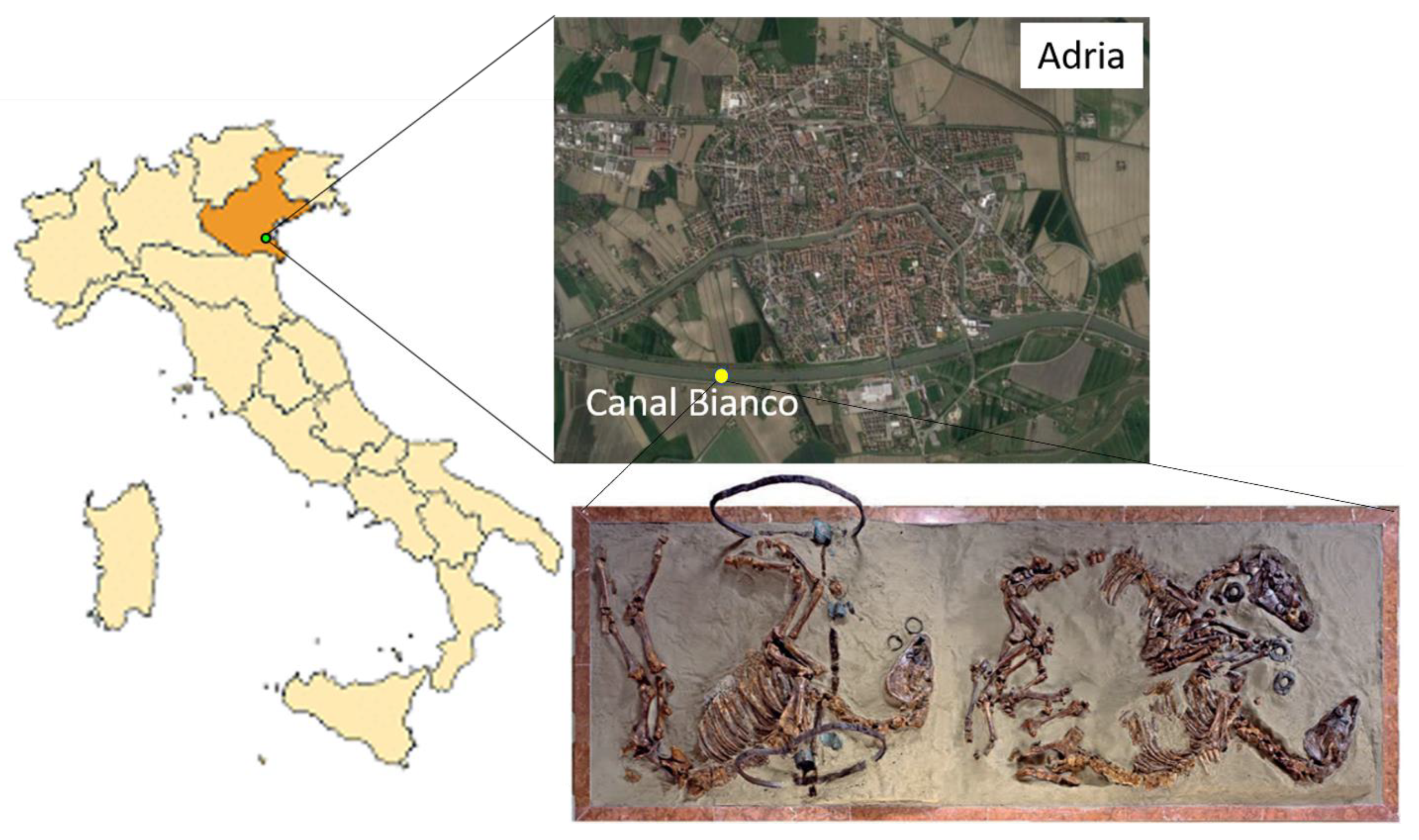
2.1. Sampling Site Description

The Tomba della Biga was found near Adria (Veneto Region, north of Italy—Figure 1) during the excavations for the new inalveation of the Canal Bianco of the city. The area was located at about 2.5 km from the river Po and ca 50 km from the current extreme point of its delta. This area was part of the Po Valley-Adriatic Sea system and also of the Alpine-Apennine and Dinaric-Hellenic promontory, an elongated basin filled with the debris of the Po River [25]. Instead, at the beginning of the third century BC, the coastline was considerably more backward.

The delta area of the Po region, in fact, preserves an accumulation of forced regressive deposits [26] that could host buried archaeological contexts emerging in correspondence with excavations and artificial depressions made for extraction purposes.

The Etruscan and Roman eras were characterized by a warm climate and fluvial stability associated with the development of a large delta in the south part of the city of Ferrara in the Emilia Romagna region, above the Veneto region [27], and a few km from the place where the Tomba della Biga was found. About 1500 years ago, the transition to wetter and cooler conditions and the relocation of the infrastructure of the Roman Empire led to an instability of the alluvial and drainage network [28] which changed the whole landscape.

2.2. Archaeological Context

A total number of 396 tombs, related to the great southern necropolis of ancient Adria, dating back to the Etruscan and Roman times, have been discovered [30]. Among these, tomb number 155 was discovered on 25 May 1938; it consists of the burial of three horses with the remains of a two-wheeled war chariot. The animals lay with a north–south orientation, two of these were coupled, lying sideways and with their heads turned towards each other; the third one remaining was placed on the chariot and resting on the right side (as you can see in the photo in Figure 1).

The bones of the three horses were analyzed by archaeo-zoologists to understand their age, sex, size, proportions, and type [31]. These authors described that two of these were male horses and a heifer thanks to the information obtained from the dentition and pubis. Concerning age, one of the male horses was probably very young (about 3 and a half years), while the heifer was the oldest (between 10 and 11 years). The horse on the chariot was about 7/8 years old; these data were obtained using Habermehl’s [32] parameters. The three horses were quite large in size: the female reached 143 cm at the withers; the adult male was slightly smaller at 140 cm, while the young horse reached 150 cm [31]. The dimensions were obtained using the Kiesewalter method [33].

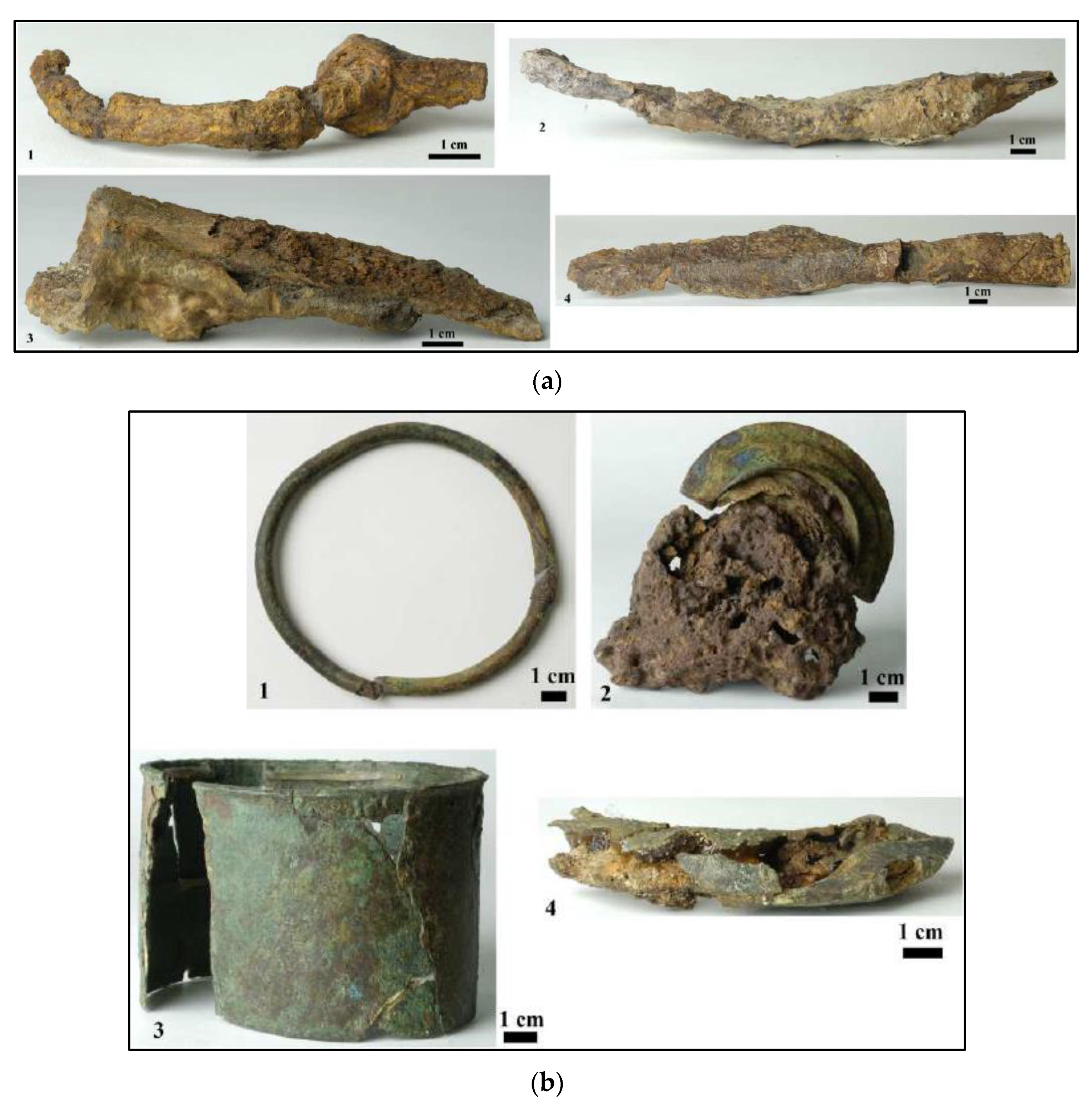
2.3. Samples Description

In this paper, 10 representative samples of the finds are characterized using a multi-analytical approach. The samples selected for the analyses were detached fragments or object edges to preserve the integrity of the sample.

Bronze fragments (i.e., sample n. 3 from pair ring; samples n. 13, 16, 20 and 25 from hubcaps) and iron fragments (samples n. 5 and 10 from axels; samples n. 1, 8 and 32 from hubcaps) have been analyzed and some of the then are shown in Figure 2.

All samples were analyzed through OLRM analysis, SEM-EDS, and µ-RS.

2.4. Analytical Techniques

Representative samples of various types of alloys were transported to the Department of Physics and Earth Sciences of the University of Ferrara for analysis.

Macroscopic investigations of the samples were carried out to define physical features (grain size, texture) and colors and to evaluate the presence of corrosion in the samples.

An observation on the surfaces of the samples was carried out using a stereomicroscope (Optika SZ6745TR) and an optical transmitted light polarized microscopy (BX51 Olympus). The optical stereomicroscope (90x total magnification) equipped with MOTICAM 2500 5.0M pixel webcam using the Motic Images Plus 2.0 ML software (version n. 2017) was used for a reflected light observation on 4 metal samples embedded into epoxy resin (3 fragments of iron 8, 10 and 32, and one of bronze, sample 3) to define their structural aspect (grain size and texture) and their state of conservation [34].

Micro-Raman spectroscopy was applied to determine the mineralogical composition of the finds without sample preparation. Micro-Raman measurements were performed using the spectrometer LabRam HR800 (Horiba Jobin Yvon, Palaiseau, France) coupled with an optical microscope Olympus BXFM (Olympus, Tokyo, Japan). The spectrometer was equipped with an air-cooled CCD, detector (1024–256 pixels) at a temperature −70 °C, which had a focal length of 80 mm and was equipped with two 600 and 1800 grooves/mm gratings. The laser beam diameter of the instrument was about 1 mm, and the resolution of the spectrometer was approximately 4 cm⁻¹. As an excitation source, we used the He–Ne laser line at 632.82 nm that was filtered to keep the laser power varying from 0.2 to 10 mW. For each sample, exposure time, beam power and accumulations were optimized in order to obtain informative spectra and to ensure to avoid sample alteration [24]. Several measurements were performed at low laser powers and increasing gradually. Raman spectra were recorded in the range of 50–2000 cm⁻¹ with an exposure time between 5 and 16 s and between 5 and 11 accumulations. The 10x and 50x microscope objectives were used to focus the laser beam onto the samples, placed on the X–Y motorized sample holder, and the spot size diameter was about 2–3 μm. The wavelength scale was calibrated using a Silicon standard (520.5 cm⁻¹) and the acquired spectra were compared with scientific published data and reference databases, such as Horiba LabSpec 5 (Horiba) and RRUFF (RRUFF, University of Arizona, Tucson, AZ, USA) [35].

Morphological and chemical characterization of the surface of the fragments was carried by a Scanning Electron Microscope (SEM) equipped with an Energy Dispersive X-ray Spectrometer (EDS) AZtec (Oxford Instruments, Abingdon, UK) for X-ray microanalysis. The SEM instrument consists of a Zeiss EVO 40 (Carl Zeiss AG, Oberkochen, Germany) with a magnification range between <5–1,000,000x and a chamber dimension 365 mm (Ø) 275 mm (h). The accelerating voltage can work from 0.2 to 30 kV. EDS analysis was carried out using air and water as the charge compensating gas, with pressures ranging from 10 Pa and 100 Pa. Electron beam energy of 20 keV and a probe current of 200 pA were used for all measurements. The SEM-EDS high magnification images of the fragment surfaces were obtained by the regulation of vacuum inside the instrument chamber with a maximum pressure of 6 Torr and performed using the SmartSEM software (Zeiss) [36]. SEM-EDS is a valuable technique to obtain information on morphology, composition, and on the pore structure of the matrix. For SEM examinations, a piece not coated with a metallic conductive layer of each fragment was firmed on an SEM stub utilizing double-sided conductive adhesive tape [37].

3. Results and Discussion

3.1. Macroscopic Characterization

All samples were first measured with a gauge in length, width, and thickness (expressed in mm), as shown in

Table 1. List of the analyzed fragments shown in the columns in order: ID of the samples, length, width, thickness, material, and origin. Dimensions were measured in millimeters.

ID sample	Length	Width	Thickness	Material	Origin
1	8	7	2	Iron	Wheels
3	8	4	1	Bronze	Pair ring
5	5	8	2	Iron	Axle
8	12	9	3	Iron	Wheels
10	9	8	6	Iron	Axle
13	9	11	1	Bronze	Hubcaps
16	7	15	1	Bronze	Hubcaps
20	5	10	1	Bronze	Hubcaps
25	6	6	1	Bronze	Hubcaps
32	26	8	2	Iron	Wheels

.

Most of the fragments were larger in longitudinal rather than the transverse direction in relation to the direction of the veins and their relationship with the maximum elongation. In addition, an internal and an external part were indicated, where possible, to reconstruct it. This criterion was not adopted for the strongly elongated iron finds collected from the wheels which, due to the strong elongation, required a horizontal placement to obtain images that represented the find in its entirety.

In detail, the iron samples are wheel rims and chariot axles. Within the fractures of the axles occur some spherules; furthermore, the thickness of the metallic part was not uniform. The fragments of the rims had similar features.

Bronze samples were represented by hubcaps and pair rings. Inside, the hubcap sample is visible with a part of the axle still engaged on the surface a patina of azurite occurs; the hubcaps show a green patina of malachite. Finally, the rings of the pair have an iron body coated with bronze (Figure 2b).

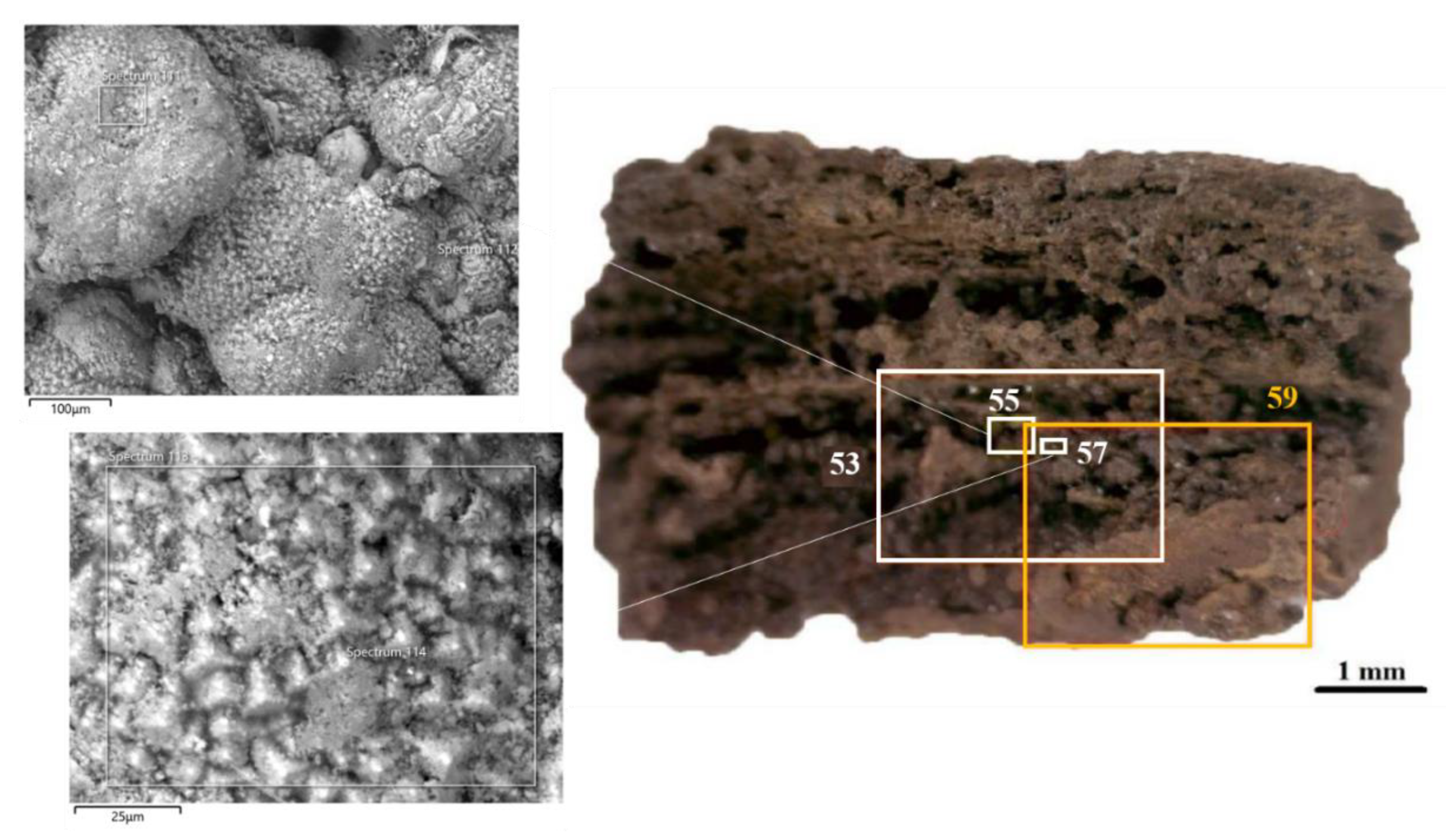
3.2. Microscopic Characterization

Structural and textural heterogeneities of the samples were defined through microscopic observations. These heterogeneities could be a consequence induced by alteration processes, fracturing and the transformation of the primary mineral phases into secondary phases (i.e., carbonates and sulphates and precipitation also of silicates) [38,39].

3.2.1. Iron Samples

Sample 1 (Figure 3a) appears clean and without crust due to the restoration. The color took on a rust-colored hue and the find was characterized by significant microstructural differences between the two sides: one part was smooth and non-porous surface, while the rear side has a scoriaceous surface (with high porosity) and is dark-colored.

Figure 3b represents sample 5. The external area is compact without porosity with an increase in the nucleation of crystals with a very fine size probably due to s metal compaction during hammering [40]. The highly elongated granules due to the deformations induced by the hammering process that flattens crystals and inclusions show elongation in the external areas, where the crystalline grain appears small and strongly elongated. The presence of fractures is filleted by alteration pores with a darker color. In addition, the external area was characterized by a rounded edge and presented a more uniform appearance of a rusty red color, probably due to iron oxides. If the metal undergoes annealing after plastic deformation, the internal structural tensions are removed, and new grains grow with regular shape [41]. If the metallic sample is produced through melting and casting processes, during the cooling phase, micro-crystals form inside the liquid mass and around these, by growth, other atoms are added that involve the formation of large crystal grains [42].

Sample 8 was characterized by the presence of green shades. The entire surface appeared to be of a rather dark rust color, tending to black, with a few exceptions that vary towards red-orange. The massive external part presents a strong iso-orientation and slight stratification; while the internal part has a granular appearance, probably due to the occurrence of gangue. It seems slightly slag-like in appearance due to the greater porosity (Figure 3g).

Sample 10 (Figure 3h) shows an irregular surface and rust color, presenting a slight stratification and variable percentage of macro-porosity. Locally it assumes a slightly scoriaceous appearance.

Sample 32 (Figure 3i) shows a dark color with some orange speckles, and it is rather irregular.

3.2.2. Bronze Samples

Sample 13 is characterized by a flat morphology (Figure 3c). The surface appears to be greenish, although it is more reddish than the other whitish areas. The size of the granules was probably influenced by the high cooling rate, which induced the nucleation of small crystals. On the front, there was a blue area, probably azurite.

Sample 16 (Figure 3c) shows a flat morphology, characterized by green shades and red copper. A marked stratification was due to structural/textural differences due to the involved production technologies. The flat outer surface exhibited corrosion that probably induced a loss of ductility and consequently an incipient macro-fracturing. In the central surface area, copper had undergone a process of alteration and transformation into copper carbonates (i.e., malachite and probably azurite). The copper core was not altered and was free of corrosion products, which characterized the metallic appearance of the sample, having the typical orange color on the front, where there was a clearly visible blue spot, presumably due to the presence of azurite in the layer, under which there seemed to be a whitish spot.

Sample 20 of Figure 3d shows the classic green patina. It presents a stratification of the microstructure as highlighted by the chromatic variations. Indeed, the green area is alternate with those red shades and/or light areas. The front of the surface presents a white spot, whereas the back area is more homogeneous, varying from green to a whitish patina. Visible from both sides was a copper-colored protrusion of the unaltered alloy.

Sample 25 (Figure 3e) shows the front surface with green and white patinas and a red central depression; the back area is presenting the same colors, but the green patina is more extensive with respect to the front. In the areas where probably malachite occurs, areas with strong chromatic variations (from light green–dark green–dark brown) are observed.

Sample 3 shows a structure very homogenous. The color changes from copper red to slight dark green shades (Figure 3f).

3.2.3. Optical Transmitted Polarized Light Both on Iron and Bronze Samples

The microstructures of the two different alloys that compose metallic elements reflect two different features. The primary characteristics are due to the heterogeneity in the composition of the metal alloy and to the presence of heterogeneously distributed impurities which modify the stability, the mineralogical and physical properties of the mineral nphases that can favor exolution processes in the solid state [43]. Some of these siderophile elements are present as sulfides.

Sample 8 is a metal alloy that shows stratification and iso-orientation of the phases probably due to the corrosion and production of different corrosion layers during burial time. The alternation of massive and non-metallic phase micro inclusion-rich layers affects rheology and deformations (Figure 4a). In the areas where they are more abundant, black microspheres and a more scoriaceous appearance is observed.

Sample 10 macroscopically shows the typical sliding bands, characteristic of ductile metals, in which the production involves deformation with thicknesses from 200 mm to 2 mm. Figure 4b shows a fine-slag microstructure with a vitreous matrix containing ferrous olivine (fayalite). Wüstite and magnetite incorporate acicular skeletal individuals of metallic iron [6]. Metallic phases can be observed within thin sub-parallel layers of irregular thickness. In some micro-domains there are remains of the original undistorted structure, in which a mixture of iron oxides and other impurities occur in forms of dendrite that precipitated at the edge of the oxide grains, which showed lower relief and hardness [44].

Sample 32 (Figure 4c) shows an alternation of dark areas surrounded by a light area. These two areas are separated by a third thin layer similar to a network. These differences are probably due to the presence of impurities. Furthermore, numerous pores are present in the coating microstructure.

Sample 3 is the only bronze sample observed and it is characterized by the occurrence of the partly preserved original alloy in the central part and two external areas with a great degree of corrosion. Based on the image it appears as though corrosion spread from external layers and along metal crystal boundaries, suggesting differences due to the metal smelting process. In addition to the main phase of the original alloy, Sn-Pb-rich phases occur. The insoluble phases, due to their different ionic potential, have different corrosive behavior which diversifies the corrosion response of the different components into the alloy. Copper products could produce an outer layer of malachite and rare azurite due to the outward migration of cations that usually characterizes copper-tin alloys.

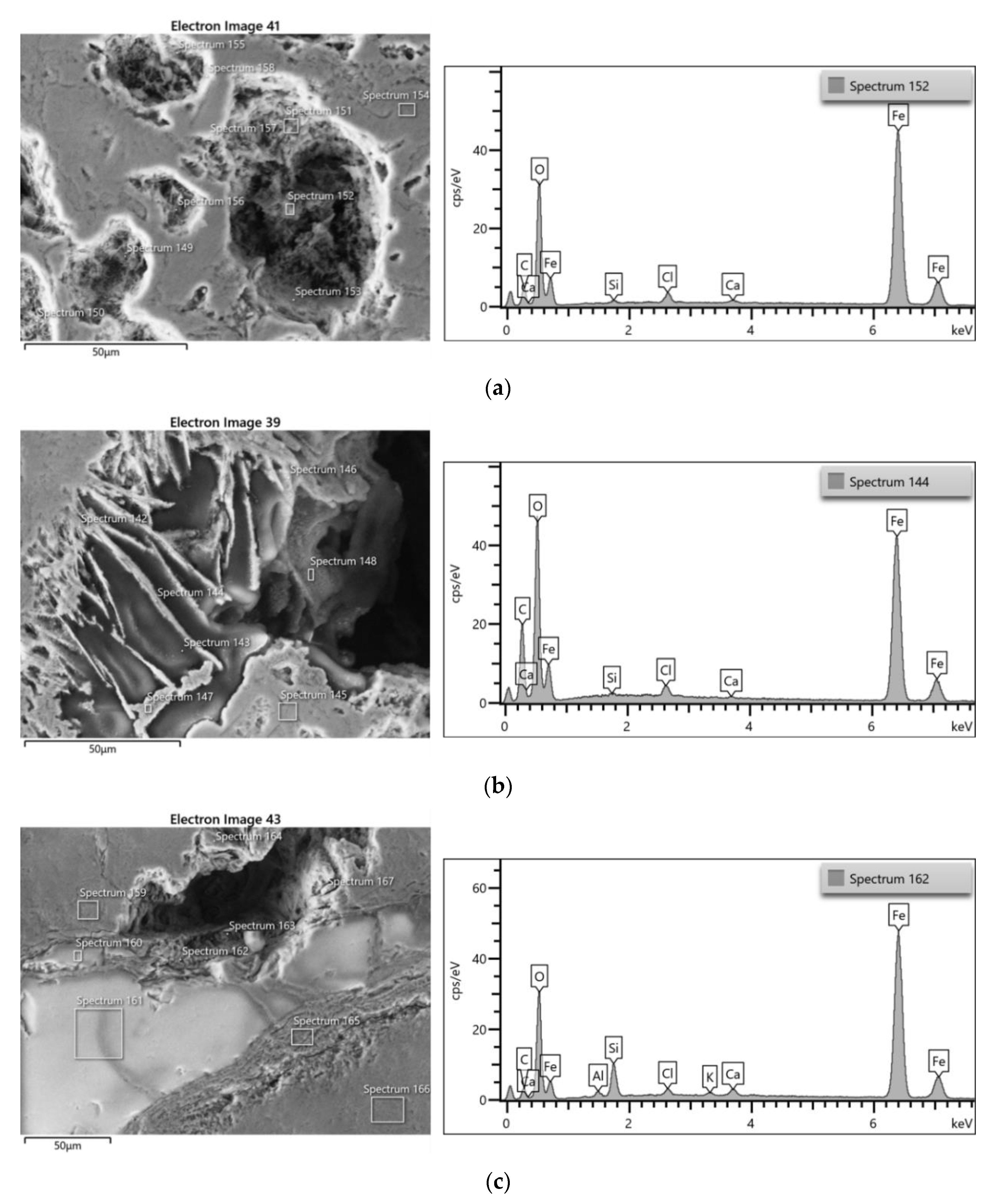
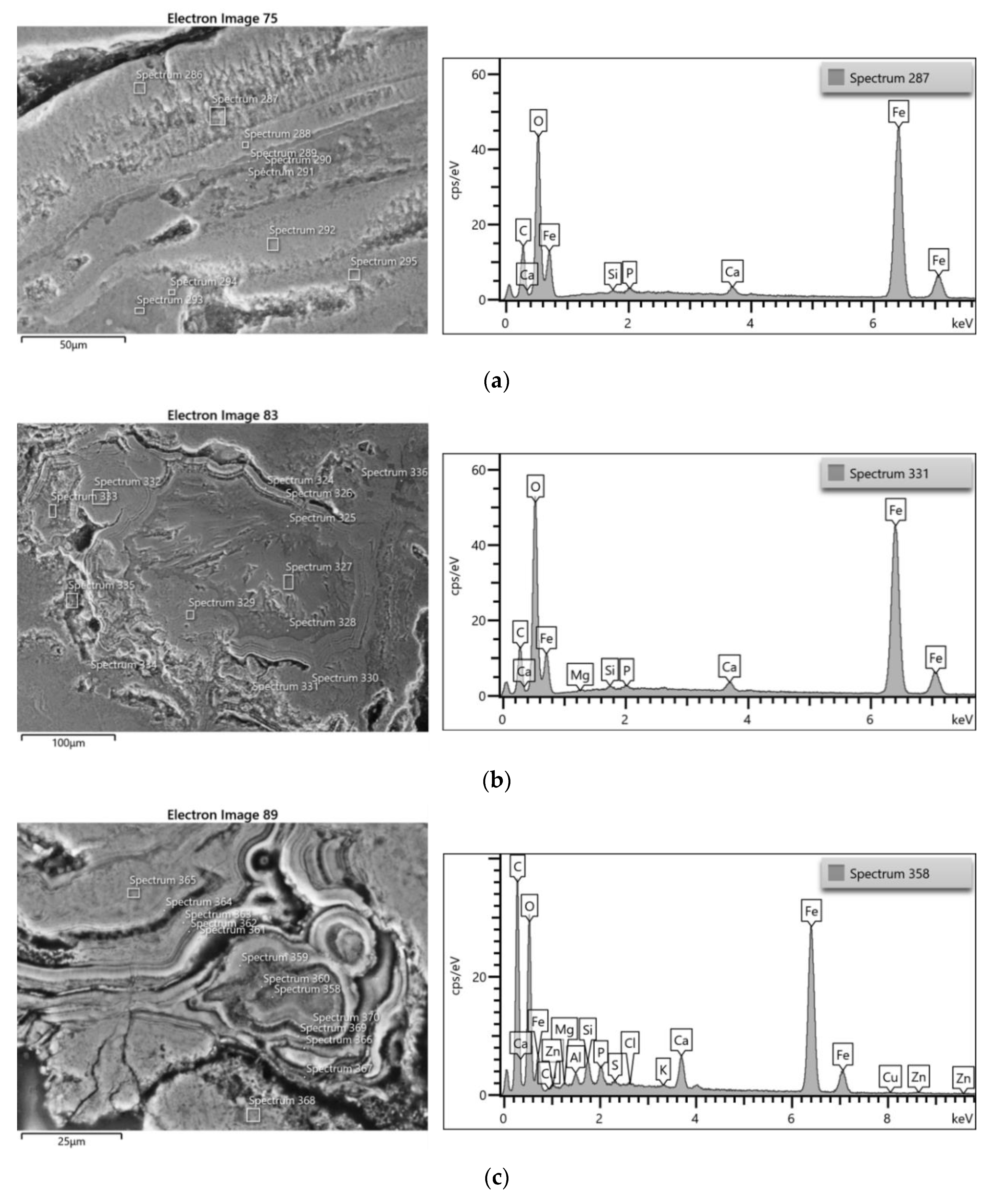
3.3. SEM-EDS Analysis

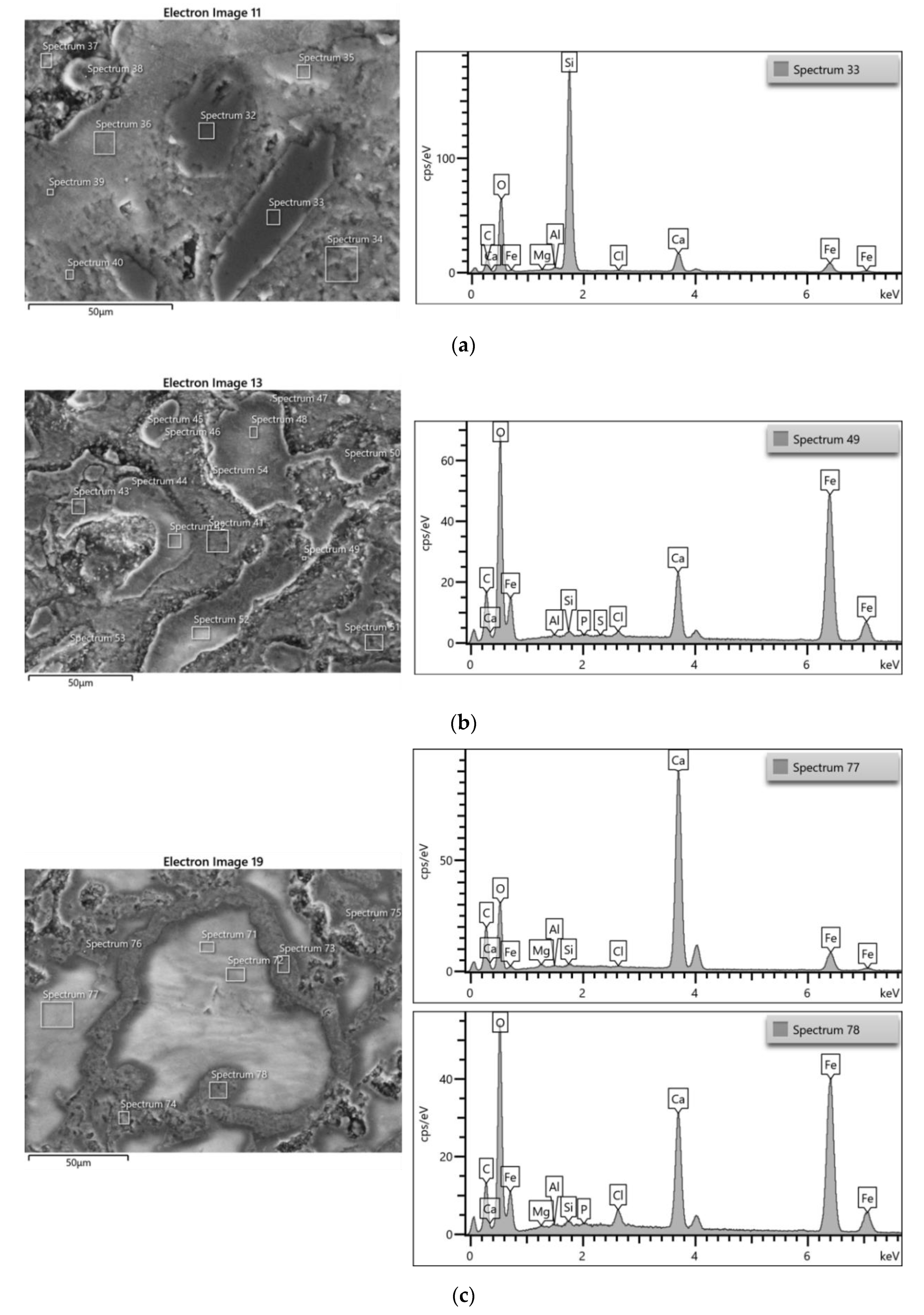
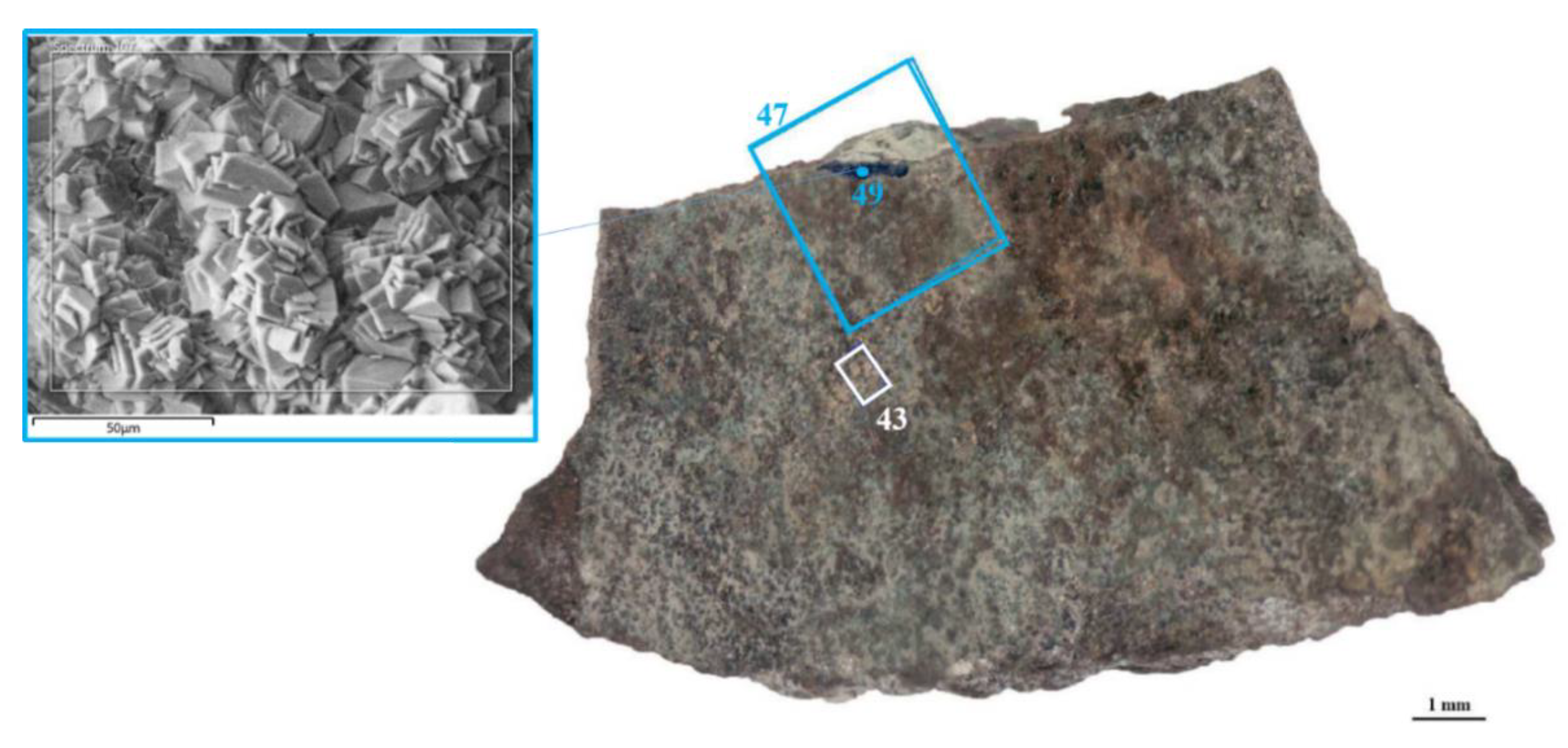
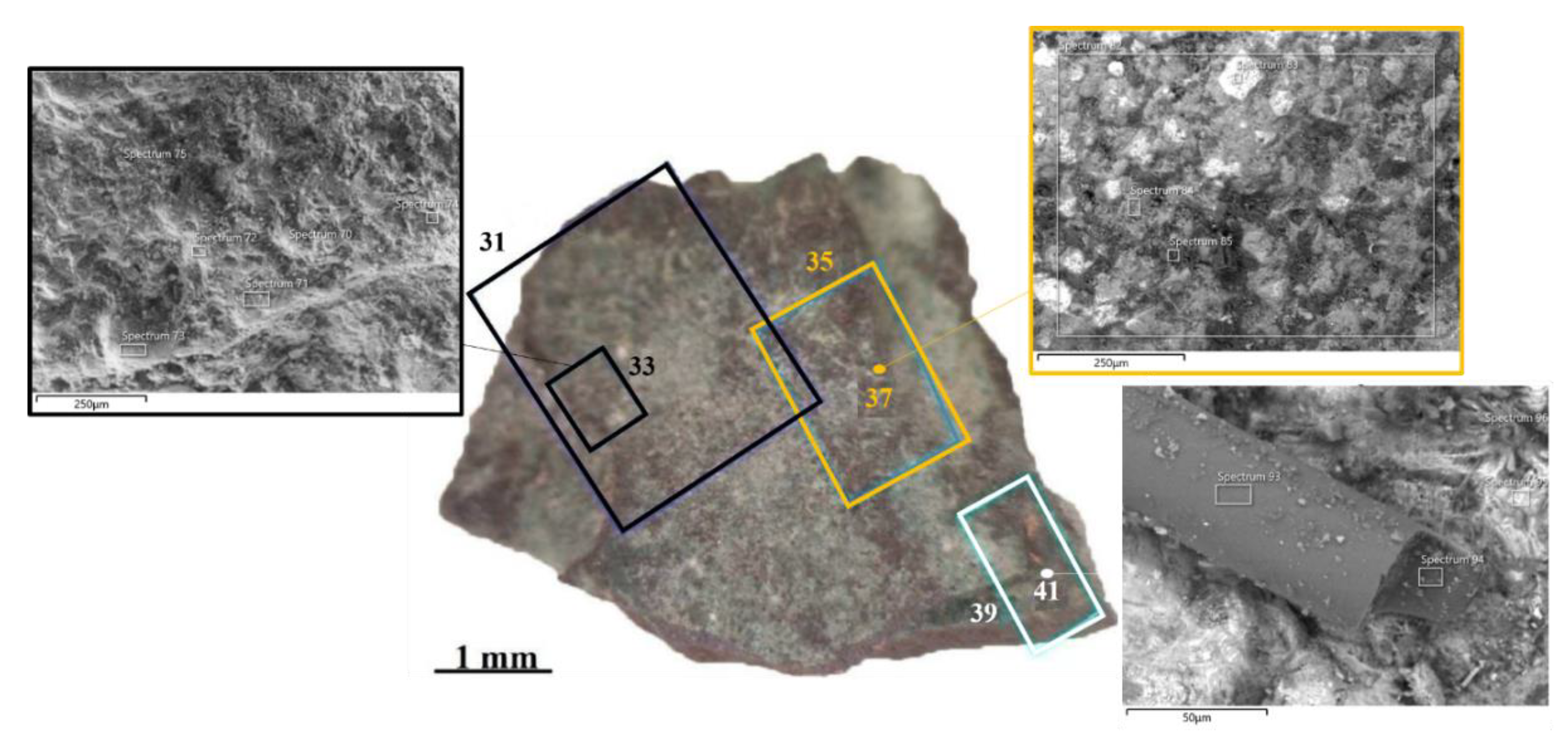
SEM investigation permitted to characterize areas with different compositions as well as to explore surfaces, patinas and bright copper stains or minerals accumulation and especially to better identify corrosion products.

In each area, numerous spectra are acquired as well as qualitative and semi-quantitative EDS analysis. The spectra obtained are a random measurement at one point (casually selected).

Table 2. SEM-EDS data analysis of all the iron samples analyzed and expressed as oxides in percentage. The second column explains the specific AREA detected in the samples. Samples 8, 10 and 32 were incorporated into the resin and sectioned. n.d. means not detected.

Iron	SiO2	Al2O3	Fe2O3	MgO	CaO	Na2O	K2O	SO2	Cl	ZnO	CuO	P2O5	Tot
sample 1	1.46	4.02	81.54	0.48	1.92	1.12	0.33	0.44	0.21	1.91	0.39	6.19	100
	0.64	2.52	82.71	0.48	1.65	0.97	0.22	0.25	0.23	2.07	0.42	7.84	100
	0.63	2.09	87.79	0.39	1.70	0.57	0.21	0.25	n.d.	1.57	0.30	4.52	100
	0.48	1.39	90.50	0.24	1.33	0.78	0.23	0.21	n.d.	1.12	n.d.	3.73	100
	0.46	0.63	93.49	0.24	0.92	0.39	0.12	0.17	n.d.	1.28	n.d.	2.31	100
	3.72	0.52	84.70	0.52	2.02	0.72	0.18	0.46	n.d.	1.77	n.d.	5.38	100
sample 5	1.79	1.70	87.54	0.30	1.07	0.77	n.d.	0.17	0.17	1.58	0.88	4.02	100
	0.99	1.63	90.94	0.25	0.67	0.61	n.d.	0.11	n.d.	1.09	0.78	2.93	100
	1.04	1.07	90.22	0.34	1.04	0.73	n.d.	n.d.	0.22	1.14	0.84	3.37	100
	0.60	7.22	89.27	0.53	0.77	n.d.	n.d.	0.13	0.13	n.d.	0.52	0.84	100
sample 8	0.20	n.d.	94.38	n.d.	0.29	n.d.	n.d.	n.d.	4.61	n.d.	n.d.	0.51	100
	0.18	n.d.	98.45	n.d.	0.17	n.d.	n.d.	n.d.	1.20	n.d.	n.d.	n.d.	100
	0.31	n.d.	98.37	n.d.	0.25	n.d.	n.d.	n.d.	1.07	n.d.	n.d.	n.d.	100
	3.81	1.27	93.15	n.d.	0.63	n.d.	0.47	n.d.	0.67	n.d.	n.d.	n.d.	100
sample 10	0.27	n.d.	98.02	n.d.	0.75	n.d.	n.d.	n.d.	n.d.	n.d.	n.d.	0.97	100
	0.22	n.d.	96.49	n.d.	1.97	n.d.	0.00	0.25	0.22	n.d.	n.d.	0.84	100
	0.34	n.d.	97.91	0.16	0.81	n.d.	n.d.	n.d.	n.d.	n.d.	n.d.	0.77	100
	2.09	1.99	87.49	0.33	2.87	n.d.	0.30	0.35	0.20	0.44	0.28	3.67	100
sample 32	70.40	1.19	20.47	0.20	7.50	n.d.	n.d.	n.d.	0.24	n.d.	n.d.	n.d.	100
	0.49	0.46	90.96	n.d.	6.87	n.d.	n.d.	0.20	0.56	n.d.	n.d.	0.46	100
	0.73	0.61	33.81	0.98	63.47	n.d.	n.d.	n.d.	0.39	n.d.	n.d.	n.d.	100
	0.46	0.41	85.93	0.19	10.97	n.d.	n.d.	n.d.	1.59	n.d.	n.d.	0.45	100
	0.56	n.d.	41.31	0.22	57.91	n.d.	n.d.	n.d.	n.d.	n.d.	n.d.	n.d.	100
	0.19	n.d.	96.33	0.00	0.67	n.d.	n.d.	n.d.	0.20	0.37	n.d.	2.24	100

and

Table 3. SEM-EDS data analysis of all the bronze samples analyzed and expressed as oxides in percentage. The second column explains the specific AREA detected in the samples. Sample 3 was incorporated into the resin and sectioned. n.d. means not detected because below the detection limit.

Bronze	SiO2	Al2O3	Fe2O3	MgO	CaO	Na2O	K2O	SO2	Cl	CuO	SnO	PbO	P2O5	Tot
sample 13	0.57	3.60	1.48	0.22	0.40	n.d.	n.d.	n.d.	0.51	89.63	3.12	0.47	n.d.	100
	0.31	2.21	0.93	n.d.	n.d.	n.d.	n.d.	n.d.	0.28	94.53	1.73	n.d.	n.d.	100
	0.21	2.97	1.57	n.d.	n.d.	n.d.	n.d.	n.d.	0.17	90.17	4.91	n.d.	n.d.	100
	0.51	2.87	3.71	n.d.	n.d.	n.d.	n.d.	n.d.	0.24	76.76	14.34	1.10	0.47	100
	0.87	2.62	2.34	0.71	2.51	n.d.	n.d.	0.19	1.65	85.26	2.95	0.48	0.43	100
	1.18	0.62	14.51	0.35	n.d.	n.d.	n.d.	n.d.	1.32	21.64	55.02	3.66	1.70	100
	1.67	1.74	23.04	0.76	1.00	n.d.	n.d.	n.d.	n.d.	20.59	44.98	3.54	2.67	100
sample 16	3.58	2.29	21.70	0.85	1.29	1.47	n.d.	0.87	1.45	26.42	33.58	3.66	2.82	100
	0.61	0.61	1.39	n.d.	0.20	n.d.	n.d.	n.d.	0.27	93.94	2.98	n.d.	n.d.	100
	0.47	0.43	1.62	n.d.	0.17	n.d.	n.d.	n.d.	0.26	91.08	2.52	0.41	3.04	100
sample 20	2.32	2.15	4.44	0.38	0.70	n.d.	0.38	1.09	1.08	82.39	4.47	n.d.	0.61	100
	1.84	1.73	4.23	0.43	0.72	n.d.	n.d.	0.37	0.60	81.84	6.79	0.81	0.64	100
	3.44	4.41	17.72	0.60	1.49	0.66	n.d.	0.75	0.29	12.53	52.08	3.65	2.38	100
	2.30	4.24	17.49	0.61	n.d.	n.d.	1.00	0.72	n.d.	9.43	57.81	4.09	2.31	100
	1.53	1.52	10.18	0.63	0.56	n.d.	n.d.	n.d.	0.24	47.16	33.71	2.76	1.71	100
	0.22	0.37	0.46	n.d.	n.d.	n.d.	n.d.	n.d.	n.d.	97.67	1.28	n.d.	n.d.	100
	0.50	0.49	3.62	n.d.	n.d.	n.d.	n.d.	n.d.	n.d.	75.77	18.24	1.37	n.d.	100
	12.33	10.48	6.36	1.50	1.32	0.37	1.77	0.25	0.17	64.34	0.45	0.36	0.29	100
sample 25	5.67	3.85	29.79	0.77	1.62	n.d.	0.47	0.80	0.51	25.18	27.59	2.09	1.65	100
	7.50	5.19	12.53	1.09	9.49	n.d.	0.70	0.98	0.35	35.50	24.89	n.d.	1.76	100
	3.99	1.12	3.87	0.56	0.73	n.d.	0.00	0.47	0.55	78.74	9.02	0.95	n.d.	100
	3.46	2.41	1.69	0.52	0.49	n.d.	0.35	0.28	0.55	89.69	0.56	n.d.	n.d.	100
	4.96	3.27	3.86	0.75	1.20	n.d.	0.46	0.80	0.42	83.56	0.72	n.d.	n.d.	100
	44.25	7.71	2.54	2.78	5.77	20.23	1.61	0.77	0.00	11.67	2.66	n.d.	n.d.	100
sample 3	0.65	n.d.	1.81	n.d.	1.15	n.d.	n.d.	0.40	0.92	94.54	0.53	n.d.	n.d.	100
	0.38	n.d.	3.06	n.d.	0.94	n.d.	n.d.	n.d.	1.53	93.75	0.34	n.d.	n.d.	100
	1.21	n.d.	8.12	0.81	1.37	n.d.	n.d.	n.d.	2.30	50.08	33.14	2.97	n.d.	100
	1.95	n.d.	15.45	n.d.	1.39	n.d.	n.d.	n.d.	1.02	67.40	6.64	1.39	4.76	100

report the SEM-EDS chemical composition related to iron samples and bronze samples, respectively, expressed as oxides in percentage.

3.3.1. Iron Samples

Sample 1. Three different macro-areas are selected to be analyzed using SEM-EDS. In each macro-area, a few smaller areas are investigated (Figure 5). SEM-EDS analyses show a homogeneous morphology of sample 1, with the presence of fractures and inclusions. The chemical composition of this sample reveals a high Fe₂O₃ content, ranging from 93.49 and 81.54 (Table 2). ZnO, CaO and P₂O₅ are also present in minor quantities with variable oxide concentrations in all analyses. SiO₂, Al₂O₃, Na₂O, MgO and SO₂ are present in low concentrations. Regarding K₂O, Cl, CuO and SO₂ the concentrations are close to the detection limit of the instrument, Pb and Sn are not detected.

Sample 5. This sample is characterized by two large areas, i.e., the surface that seems unaltered and the excavated area containing some spherules (Figure 6). The sample has a porous morphology. The content of Fe₂O₃ varies from 87.54 to 90.94 (Table 2). Low concentrations of SiO₂, Al₂O₃, Na₂O and MgO are observed as suggested by the intensity of their peaks resulting in a similar composition to that of sample 1. In addition, P₂O₅ is present in all the analyses with a maximum value of 4.02, CaO with a value close to 1. The metals ZnO and CuO were present, as well as CaO. Sulphur and Cl have concentrations close to the detection limit of the instrument. Pb and Sn are not detected.

In the samples incorporated into the resin and sectioned (samples 8, 10 and 32), different spectra were analyzed for each area selected, but the paper showed only the representative spectra for each analyzed area. All the samples were not characterized by metal elements such as Cu, Zn, Sn and Pb.

Sample 8 was characterized by a high value of Fe oxide in all the parts of the sample analyses, as shown in the spectra of Figure 7 and in Table 2. Aluminum, Si, P, Cl, K and Ca oxides were observed but with very low values. Na, Mg, S and the metals Cu, Zn, Sn and Pb oxides were not detected or were very close to the detection limit of the instrument.

Sample 10. Figure 8 showed SEM images of the analyzed areas; the sample appeared with a homogenous morphology with small fractures. The chemical composition reported a high value of Fe₂O₃, close to sample 8, especially in the first three EDS-spectra that ranged from 96.49 to 98.02 (Figure 8a,b and Table 2). Only the spectrum of Figure 8c showed a lower value of Fe with respect to the other spectra (87.49) and a very low amount of Cu and Zn oxides. In all the spectra, Mg, Al, Si, P, S, Cl, K and Ca oxides occurred in very low values. Na, Sn and Pb oxides were not detected.

Sample 32. SEM images and EDS analyses were shown in Figure 9, in which the sample appeared with a homogenous morphology with small fractures, as for the sample previously described. The chemical composition was very similar to the previous sample analyzed with high values of Fe₂O₃ with a maximum value of 96.33 (Table 2). The other three spectra were characterized by lower values of Fe₂O₃, but high values of Ca. Mg, Al, P, S and Cl oxides were observed but with very low values. Na, K, and the metals Cu, Zn, Sn and Pb oxides were not detected.

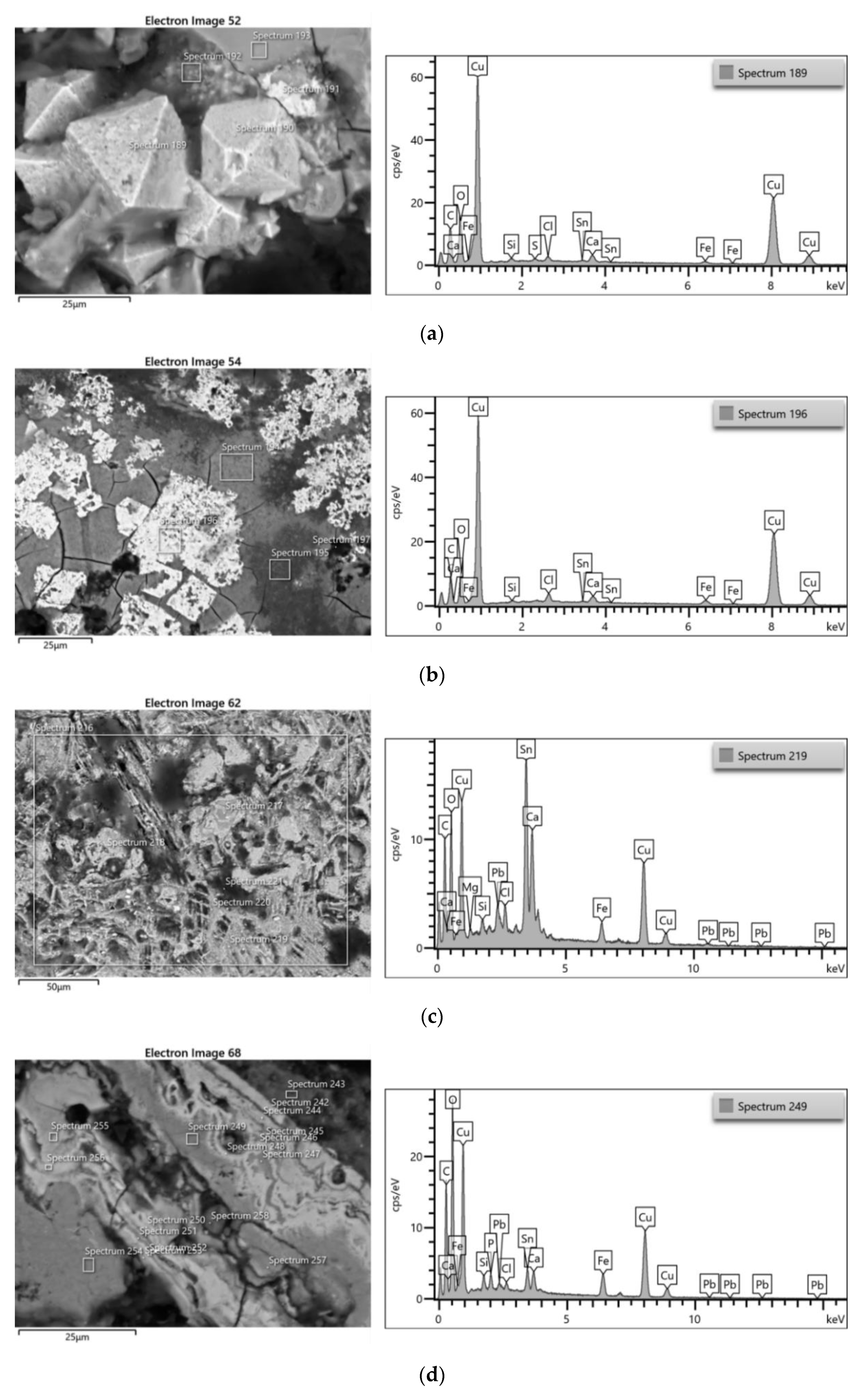
3.3.2. Bronze Samples

Sample 13. The investigations are mainly focused on one area, which seems to have impurities (Figure 10 on the left). The morphology is homogenous and completely different from the other two samples previously described. However, different kinds of inclusions infer differences in color on the surface. The most abundant oxide is CuO which varies from 20.59 to 94.53 (Table 3), depending on the analyzed areas. SnO is also present with quite high values (from 1.73 up to 55.02). It was interesting to note that in areas 11 and 13 where CuO is low, SnO has high values and vice versa. Fe₂O₃ shows low concentration, followed by Al₂O₃. Si, Mg, P, S, Cl and K oxides have concentrations close to the detection limit of the instrument. Lead occurs in very low amounts and not in all spectra. In this case, Na and Zn oxides are not detected.

Sample 16. Figure 11 shows the scheme of the analyzed areas and the photo imaging. The morphology appears homogenous in most of the sample, as for sample 13. The imaging of detail 49 (in light blue) was interesting, in which differences in color on the surface of the samples are visible, probably due to the presence of different kinds of inclusions. CuO is the major oxide, ranging from 26.42 to 93.94. SnO is also present with high content, especially in area 43, where it reaches the highest values (33.58). On the contrary, CuO has the lowest value (26.42 respect to 93.94 and 91.08 of the other area analyzed), as for sample 13. Always in area 43, PbO occurs with high values (3.66) and high values of Fe₂O₃ (21.70), instead, both had lower values in the other two areas. Na, Mg, Al, P, S, Cl and also Si and Ca oxides have concentrations close to the detection limit of the instrument. K and Zn oxides were not detected.

Sample 20. This fragment was extensively investigated, starting from the area on the right including the green patina and an underlying orange from which we could see the underlying layer (Figure 12). SEM images showed a homogenous morphology of the sample. CuO is the most abundant oxide (Table 3) with a maximum value of 97.67, but in some areas analyzed the presence of CuO was lower (9.43 or 12.53). In the areas where low values of CuO occur, high values of SnO are observed (52.08 and 57.81, respectively). Fe₂O₃ was also analyzed in all the areas, showing a heterogeneous distribution. Na, Mg, P, S, Cl, K and Ca oxides have concentrations close to the detection limit of the instrument. Si and Al oxides occur in very low values content, excluding the results of area 29. Zn was not detected.

Sample 25. Figure 13 shows the scheme of the analyzed sample. The morphology observed through the photo imaging at the SEM microscope showed a homogenous sample. This sample was mainly composed of CuO (Table 3) characterized by high variability of weight oxide (from 11.67 to 89.69). In areas in which CuO was prevalent, the presence of SnO was lower and vice versa. Si and Al oxides were observed at low-value percentages except for the area 41 (44.25 and 7.71, respectively), which was also characterized by anomalous high values of Na₂O (20.23 as shown in Table 3) and CaO (5.77). CaO was also present with high values (9.49) in area 33. Area 31 was characterized by the highest value of SnO (27.59), Fe₂O₃ (29.79) and PbO (1.65). Fe₂O₃ was also observed in all the other areas analyzed but with lower values, instead of PbO only in two areas. Mg, P, S, Cl and K oxides were observed but with very low-value percentages. Zn was not detected.

Sample 3. In sample n. 3, incorporated into the resin and sectioned, different spectra were analyzed for each area selected, but the paper showed only the representative spectra for each analyzed area. Figure 14 shows SEM images and EDS spectra of the representative areas analyzed. Figure 14a shows particles with a regular morphology characterized by high values of CuO (94.54, as shown in Table 3). The spectrum of Figure 14b was similar to the previous one. The spectrum of Figure 14c shows high contents of CuO (50.08) and SnO (33.14) and small quantities of Fe₂O₃ (8.12). Similar but not equal was the spectrum of Figure 14d, with similar values of Fe and Pb oxides. These two last spectra shown also small values of PbO (2.97 and 1.39, respectively). Mg, Si, P, S and Cl oxides were observed but with very low values. Na, Al, K and Zn oxides were not detected.

The scarce presence of Cl, S and P species as the main corrosion agents in most of the samples, both iron and copper, justifies the low degree of corrosion due to environmental agents. Although the excavation area is close to the coastline and the aquifer is affected by the ingression of saltwater, the presence of clay sediments has protected the artifacts from corrosion and the concentration of chlorine detected is very low so that the metal was protected from corrosion [45].

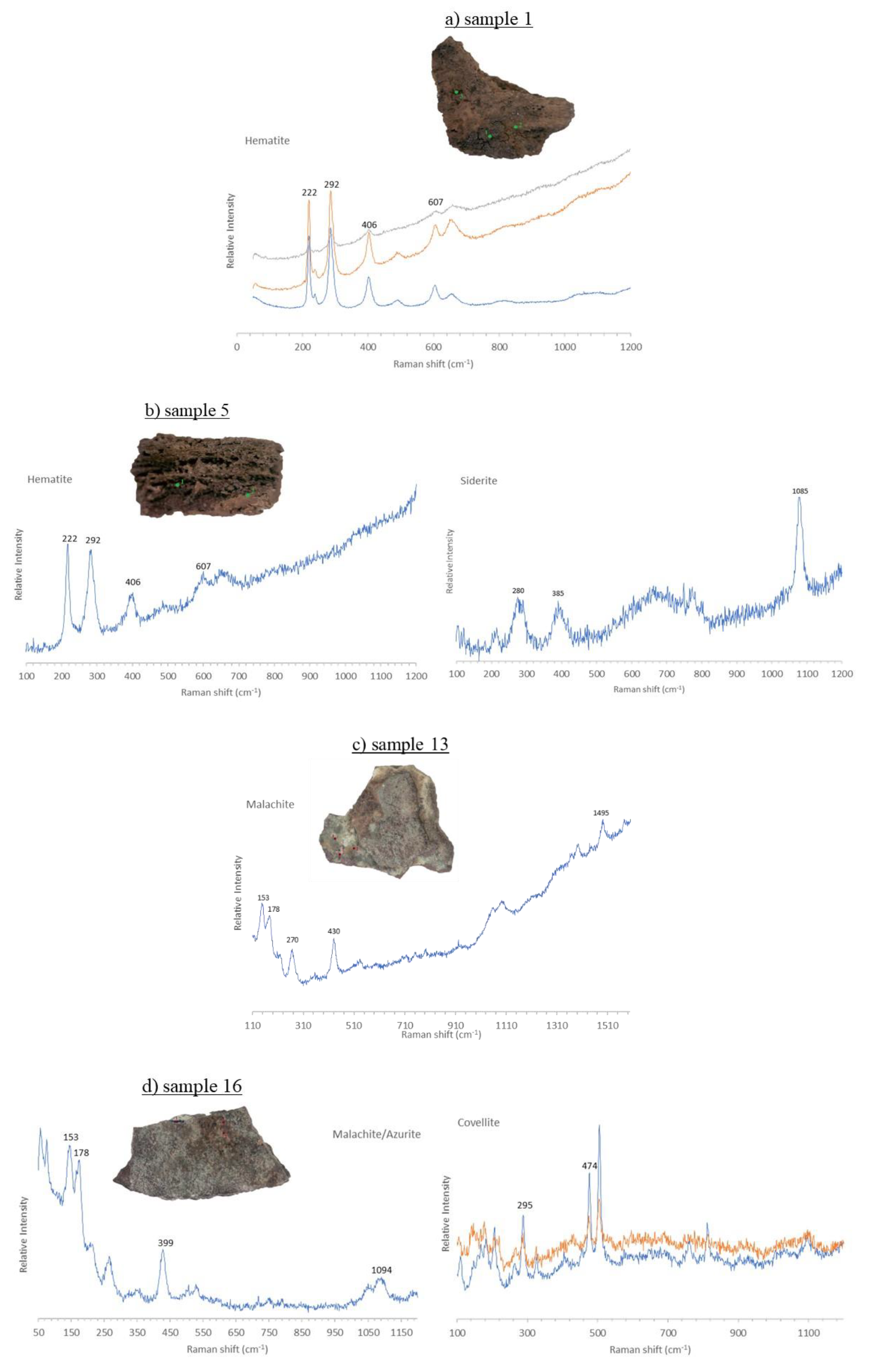
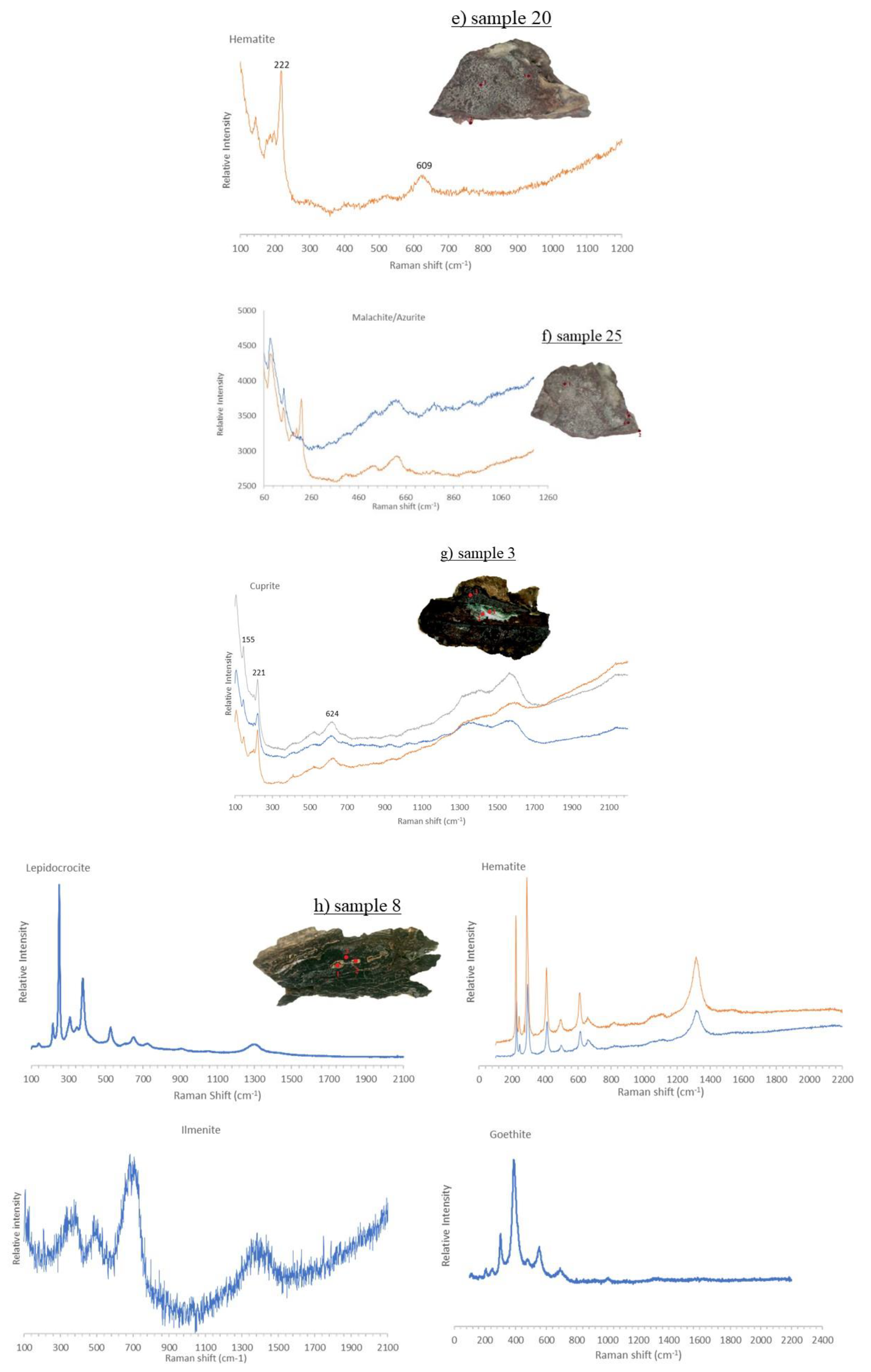
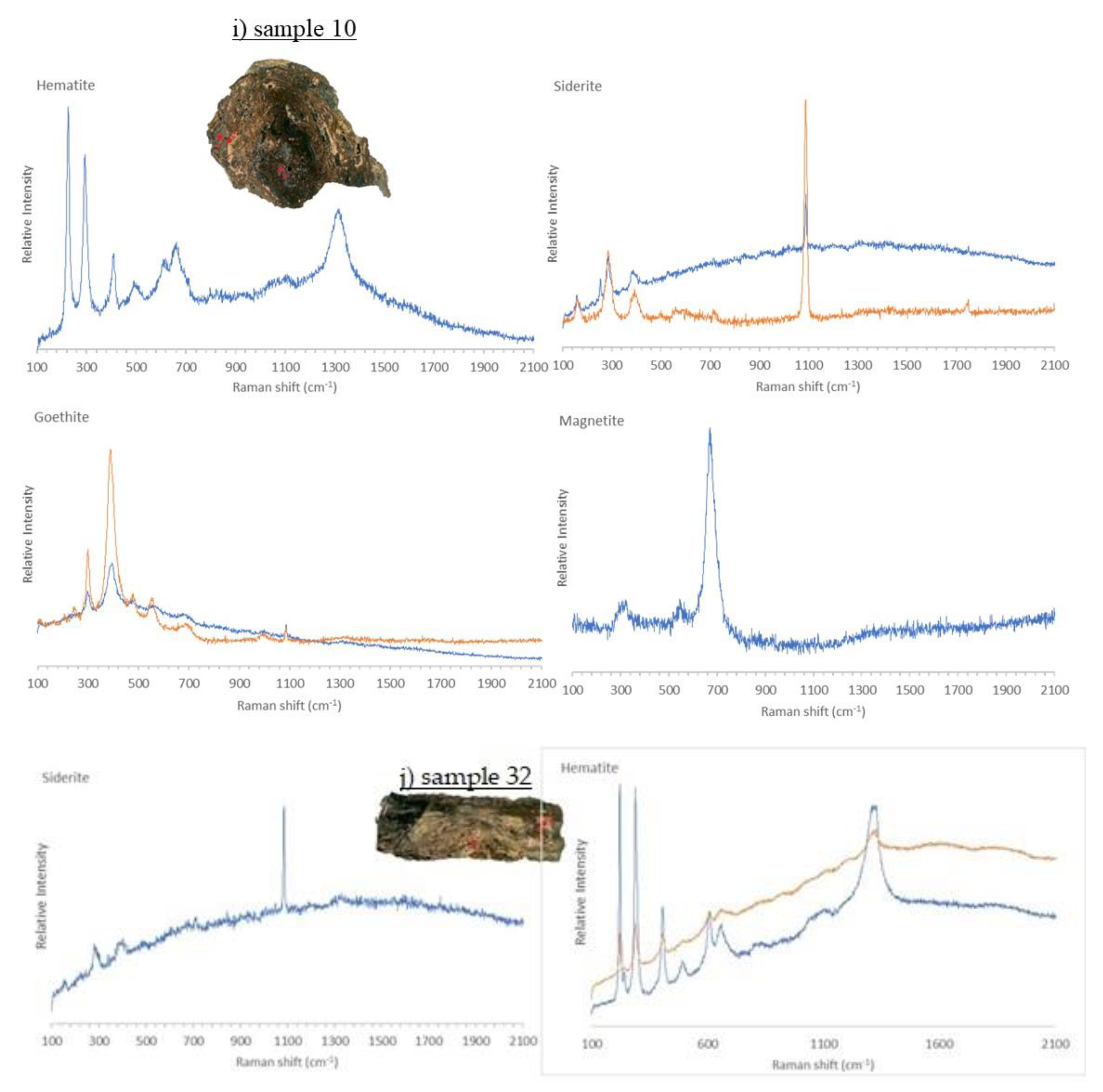
3.4. Micro-Raman Spectroscopy

Micro-Raman spectroscopy was used to explore the mineralogy of all samples. In order to choose the points to investigate, in this case, chromatic differences are used and probing the samples in several points. For each sample different spectra were analyzed, each spectrum represents a different point (e.g., point 1 represents spectrum 1 and so on).

3.4.1. Iron Samples

For the iron samples, Raman confirmed the presence of iron oxides (hematite and magnetite), iron hydroxides (goethite) and ferrous carbonate (siderite).

In detail, sample 1 was investigated in three different areas: the first in the most fractured and dark area, the second on the surface with a less altered appearance and the third with the attempt to identify the restored and repaired area with the resin (Figure 15a). The spectra show that the majority part of the sample is composed of hematite (Fe₂O₃) [46].

Figure 15b shows the spectra acquired on sample 5. The two analyses are made on spherules and unaltered surfaces, respectively. The first spectrum suggests the occurrence of a red pigment similar to hematite, while the second is the presence of siderite (FeCO₃) [47].

The center of sample 8 is characterized by light spots than the rest of the sample. Spectrum 1 shows goethite (Fe⁺³O(OH)) [48], spectrum 2 lepidocrocite [49], while spectrum 3 corresponded to ilmenite (Figure 15c).

Starting from the outside, different areas were investigated in sample 10 (as shown in Figure 15d): a grey-green part (point 1), a lighter one tending to beige (point 2) and a rust-colored area (point 3). Spectrum 1 was represented by magnetite (Fe₃O₄) [46], while spectrum 2 goethite and finally spectrum 3 siderite.

Figure 15e shows the micro-Raman results related to the last sample 32. The first area selected (point 1) had been identified in the center of the fragment in a beige area, while the second was located in an area with similar color but more homogeneous. Finally, the third point was chosen close to the previous one but in a grey area. The last sample did not show new results; also, in this case, spectrum 1 was characterized by hematite, while all the other investigated areas contain siderite (spectrum 2) and goethite (spectrum 3).

3.4.2. Bronze Samples

With regard to the bronze finds (alloy formed by copper and tin), Raman spectra showed the constant presence of magnetite and goethite, suggesting the important role of these minerals in the preservation of the metallic finds against alteration and decay [50].

In detail, in sample 13, the first area analyzed is characterized by a green patina, followed by a second area characterized by orange color and then the copper-colored area (Figure 15f). The spectra show that the first sampled point contains malachite (Cu₂(CO₃)(OH)₂) [51].

Instead, in sample 16, the first area analyzed was the blue area, followed by the orange area in the upper area on the right. The blue zone is composed of azurite (Cu₃(CO₃)₂(OH)₂) [51]. The last points probably correspond to covelite (CuS) (Figure 15g) [52].

Figure 15h show the spectra acquired on sample 20, in which three different areas are analyzed, i.e., the green patina, the copper-colored layer and the orange patina, respectively. The spectra confirmed the presence of hematite.

Sample 25 was analyzed in four different areas, the first on the green patina in the upper area, the second at the lower right and in the rust-colored area, the third slightly higher but in a green part and the last one on the copper-colored surface. Unfortunately, it was not possible to distinguish three of the chosen trends, while the first confirmed the presence of malachite (Figure 15i).

The first and interesting peculiarity that characterizes sample 3 is the green patina that varies towards white (first spectrum) inside the sample (Figure 15j). Instead, spectrum 2 represented a raised dark rust-colored area, almost black (second spectrum). Both spectra revealed the presence of copper: the green patina could be cuprite [53,54] and the white part probably siderite, while spectrum 3 revealed copper oxide.

4. Conclusions

This research based on the minero-petrographic approach permitted to acquire knowledge on the materials used for the production of metallic finds unearthed in the ancient city of Adria (north of Italy).

The study showed the occurrence of two main alloys, one Fe and the other Cu-Sn bronze. The data highlighted that the alloys have important corrosion evidence.

The concentration of impurities in the Fe alloy is very low, some transition metals are below the detection limits for SEM-EDS. The constant presence of Cl and Na could be related to the coastal environment of the sampling site, which probably indicated an interaction with brackish waters that possibly had partially affected the degree of conservation.

Regarding the Cu-Sn alloy, a strong variation in the ratio of the two metals was observed due to the greater mobility of copper. However, during the corrosive process decuprification and/or destannification processes can be involved, leading to selective enrichment/depletion.

The Fe₂O₃ content was high, justifying the observed fracturing in the artifacts. SiO₂ was also present in a very low concentration, while Al₂O₃ was present in slightly higher concentrations. The percentage of sulfur was low, so sulphates were rare.

Several factors influenced the rheology and the manufacturing processes as shown by ORLM on four selected samples. In fact, metallographic properties had been identified for the two types of alloys linked to the degree of slagging and purification of the alloy, to the raw materials and to the technology used in the shaping. These variations and anisotropies probably influenced the corrosion of the archaeological iron, and the study could give suggestions for the development plan of conservation strategies. The petrographic study and SEM analyses made it possible to identify the chemism of the phases whose mineralogical nature was confirmed with micro-Raman microanalysis.

Despite the long period of burial conditions, in an unfavorable context, the metallic finds showed a state of conservation high as the structural and textural elements of the original alloys are still preserved.

The analytical techniques used in this research work allow differentiating corrosion products evaluating the state of conservation of the metallic finds of the Tomba della Biga, which is an important cultural heritage for the city of Adria and its population.

References

1. Giblin, J.I.; Knudson, K.J.; Bereczki, Z.; Palfi, G.; Pap, I. Strontium isotope analysis and human mobility during the Neolithic and Copper Age: A case study from the Great Hungarian Plain. J. Archaeol. Sci. 2013, 40, 227–239. [Google Scholar] [CrossRef]
2. Greenfield, H.; Marciniak, A. Retention of old technologies following the end of the Neolithic: Microscopic analysis of the butchering marks on animal bones from Çatalhöyük East. World Archaeol. 2019, 51, 76–103. [Google Scholar] [CrossRef]
3. Dolfini, A. From the Neolithic to the Bronze Age in Central Italy: Settlement, Burial, and Social Change at the Dawn of Metal Production. J. Archaeol. Res. 2020, 28, 503–556. [Google Scholar] [CrossRef] [Green Version]
4. Pearce, M. The ‘Copper Age’—A History of the Concept. J. World Prehistory 2019, 32, 229–250. [Google Scholar] [CrossRef] [Green Version]
5. Sun, Y.; Muta, H.; Kurosaki, K.; Ohishi, Y. Thermal and Electrical Conductivity of Liquid Al-Si Alloys. Int. J. Thermophys. 2019, 40, 31. [Google Scholar] [CrossRef]
6. Huang, M.; Xu, C.; Fan, G.; Maawad, E.; Gan, W.; Geng, L.; Lin, F.; Tang, G.; Wu, H.; Du, Y.; et al. Role of layered structure in ductility improvement of layered Ti-Al metal composite. Acta Mater. 2018, 153, 235–249. [Google Scholar] [CrossRef]
7. Ayedun, F.; Adebambo, P.O.; Adetunji, B.I.; Ozebo, V.C.; Oguntuase, J.A.; Adebayo, G.A. Increased Malleability in Tetragonal Zrx Ti1−x O2 Ternary Alloys: First-Principles Approach. Z. Nat. A 2017, 72, 567–572. [Google Scholar] [CrossRef]
8. Hauptmann, A. Making Metals: Ancient Metallurgical Processes. In Archaeometallurgy—Materials Science Aspects; Natural Science in Archaeology; Springer: Cham, Switzerland, 2020. [Google Scholar] [CrossRef]
9. Artioli, G.; Canovaro, C.; Nimis, P.; Angelini, I. LIA of Prehistoric Metals in the Central Mediterranean Area: A Review. Archaeometry 2020, 62, 53–85. Available online: https://publons.com/publon/10.1111/arcm.12542. (accessed on 7 November 2022).
10. Liss, B.; Levy, T.E.; Day, J.M.D. Origin of iron production in the Eastern Mediterranean: Osmium isotope and highly siderophile element evidence from Iron Age Jordan. J. Archaeol. Sci. 2020, 122, 105227. [Google Scholar] [CrossRef]
11. Ingo, G.M.; Riccucci, C.; Pascucci, M.; Messina, E.; Giuliani, C.; Fierro, G.; Di Carlo, G. Integrated analytical methodologies for the study of the corrosion products naturally grown on Roman Ag-based artefacts. Appl. Surf. Sci. 2018, 446, 279–286. [Google Scholar] [CrossRef]
12. Gambacurta, G.; Tirelli, M. Le Sepolture di Cavallo Nella Necropoli “Le Brustolade”. La Protostoria tra Sile e Tagliamento. Antiche Genti tra Veneto e Friuli, Catalogo Della Mostra; Esedra: Padova, Italy, 1996; pp. 71–74. [Google Scholar]
13. Robbiola, L.; Vilbert, D.; Lejars, T.; Bourgarit, D.; Mille, B. Characterization of a buried archaeological bronze from the Celtic tomb n°1002 of La Fosse Cotheret (Roissy-en-France). Metal 2001, 237–242. [Google Scholar]
14. Gerwin, W.; Baumhauer, R. Effect of soil parameters on the corrosion of archaeological metal finds. Geoderma 2000, 96, 63–80. [Google Scholar] [CrossRef]
15. Bernabale, M.; Nigro, L.; Vaccaro, C.; Nicoli, M.; Montanari, D.; Bigini, P.; De Vito, C. Micro-Raman spectroscopy and complementary techniques for the study of iron weapons from Motya and Lilybaeum (Sicily, Italy): Corrosion patterns in lagoon-like and calcarenitic hypogea environments. J. Raman Spectrosc. 2022, 53, 272. [Google Scholar] [CrossRef]
16. Jia, M.; Hu, P.; Hu, G. Corrosion Layers on Archaeological Cast Iron from Nanhai I. Materials 2022, 15, 4980. [Google Scholar] [CrossRef]
17. Ashkenazi, D. How can fracture mechanics and failure analysis assist in solving mysteries of ancient metal artifacts? Archaeol. Anthropol. Sci. 2020, 12, 34. [Google Scholar] [CrossRef]
18. Vietti, A.; Angelini, E.; Grassini, S.; Donato, N. Raman spectroscopic characterization of corrosion products of archaeological iron. J. Phys. Conf. Ser. 2022, 2204, 012066. [Google Scholar] [CrossRef]
19. Liang, Z.; Jiang, K.; Zhang, T. Electrochemical and passive behaviour of Cu–Sn bronze in simulated archaeological soil media. Mater. Corros. 2021, 72, 743–756. [Google Scholar] [CrossRef]
20. Liang, Z.; Jiang, K.; Zhang, T. Corrosion behaviour of lead bronze from the Western Zhou Dynasty in an archaeological-soil medium. Corros. Sci. 2021, 191, 109721. [Google Scholar] [CrossRef]
21. Neff, D.; Bellot-Gurlet, L.; Dillmann, P.; Reguer, S.; Legrand, L. Raman imaging of ancient rust scales on archaeological iron artefacts for long-term atmospheric corrosion mechanisms study. J. Raman Spectrosc. 2006, 37, 1228–1237. [Google Scholar] [CrossRef]
22. Mercier-Bion, F.; Li, J.; Lotz, H.; Tortech, L.; Neff, D.; Dillmann, P. Electrical properties of iron corrosion layers formed in anoxic environments at the nanometer scale. Corros. Sci. 2018, 137, 98–110. [Google Scholar] [CrossRef]
23. Oudbashi, O. A methodological approach to estimate soil corrosivity for archaeological copper alloy artefacts. Herit. Sci. 2018, 6, 2. [Google Scholar] [CrossRef]
24. Ingo, G.M.; Riccucci, C.; Guida, G.; Pascucci, M.; Giuliani, C.; Messina, E.; Fierro, G.; Di Carlo, G. Micro-chemical investigation of corrosion products naturally grown on archaeological Cu-based artefacts retrieved from the Mediterranean sea. Appl. Surf. Sci. 2019, 470, 695–706. [Google Scholar] [CrossRef]
25. Amorosi, A.; Maselli, V.; Trincardi, F. Onshore to offshore anatomy of a late Quaternary source-to-sink system (Po Plain-AdriaticJia Sea, Italy). Earth Sci. Rev. 2016, 153, 212–237. [Google Scholar] [CrossRef]
26. Stefani, M. The Po Delta Region: Depositional Evolution, Climate Change and Human Intervention through the Last 5000 Years. In Landscapes and Landforms of Italy; World Geomorphological Landscapes; Soldati, M., Marchetti, M., Eds.; Springer: Cham, Switzerland, 2017. [Google Scholar] [CrossRef]
27. Stefani, M.; Vincenzi, S. The interplay of eustasy, climate and human activity in the late Quaternary depositional evolution and sedimentary architecture of the Po Delta system. Mar. Geol. 2005, 222–223, 19–48. [Google Scholar] [CrossRef]
28. Bruno, L.; Amorosi, A.; Curina, R.; Severi, P.; Bitelli, R. Human–landscape interactions in the Bologna area (northern Italy) during the mid-late Holocene, with focus on the Roman period. Holocene 2013, 23, 1560–1571. [Google Scholar] [CrossRef]
29. Gambacurta, G. Adria. Museo Archeologico Nazionale di Adria. Guide Tematiche dei Musei Archeologici del Veneto; Tiné V. La Tipografica srl: Udine, Italy, 2013. [Google Scholar]
30. Bonomi, S.; Zega, L. La Sezione Etrusca: Adria e il Basso Polesine tra i Secoli VI e il III a.C.; Ministero per i beni e le Attività Culturali, Soprintendenza per i Beni Archeologici del Veneto, Apogeo Editore: Milano, Italy, 2008. [Google Scholar]
31. Reggiani, P.; Rizzi Zorzi, J. I cavalli della Tomba della Biga conservata al Museo archeologico nazionale di Adria (RO). Atti del 4° Convegno Nazionale di Archeozoologia, Quaderni del Museo archeologico del Friuli Occidentale; Malerba, G., Visentini, P., Eds.; Pordenone, Italy, 2003; 6, pp. 315–322. Available online: https://www.researchgate.net/publication/330638801_I_cavalli_della_Tomba_della_Biga_conservata_al_Museo_Archeologico_Nazionale_di_Adria_RO. (accessed on 7 November 2022).
32. Habermehl, K.H. Die Altersbestimmungbei Hais-und Labortieren; Parey: Berlin, Germany, 1975. [Google Scholar]
33. Chrószcz, A.; Baranowski, P.; Janowski, A.; Poradowski, D.; Janeczek, M.; Onar, V.; Sudoł, B.; Spychalski, P.; Dudek, A.; Sienkiewicz, W.; et al. Withers height estimation in medieval horse samples from Poland: Comparing the internal cranial cavity based modified Wyrost and Kucharczyk method with existing methods. Int. J. Osteoarchaeol. 2022, 32, 378–395. [Google Scholar] [CrossRef]
34. Marrocchino, E.; Telloli, C.; Pedrini, M.; Vaccaro, C. Natural stones used in the Orsi-Marconi palace façade (Bologna): A petro-mineralogical characterization. Heritage 2020, 3, 1109–1123. [Google Scholar] [CrossRef]
35. Rosina, P.; Collado, H.; Garces, S.; Comes, H.; Eftekhari, N.; Nicoli, M.; Vaccaro, C. Benquerencia (La Serena—Spain) rock art: An integrated spectroscopy analysis with FTIR and Raman. Heliyon 2019, 5, e02561. [Google Scholar] [CrossRef] [Green Version]
36. Telloli, C.; Chicca, M.; Pepi, S.; Vaccaro, C. Saharan dust particles in snow samples of Alps and Apennines during an exceptional event of transboundary air pollution. Environ. Monit. Assess. 2018, 109, 37. [Google Scholar] [CrossRef]
37. Marrocchino, E.; Telloli, C.; Caraccio, S.; Guarnieri, C.; Vaccaro, C. Medieval Glassworks in the City of Ferrara (North Eastern Italy): The Case Study of Piazza Municipale. Heritage 2020, 3, 819–837. [Google Scholar] [CrossRef]
38. Portillo, H.; Zuluaga, M.C.; Ortega, L.A.; Alonso-Olazabal, A.; Murelaga, X.; Martinez-Salcedo, A. XRD, SEM/EDX and micro-Raman spectroscopy for mineralogical and chemical characterization of iron slags from the Roman archaeological site of Forua (Biscay, North Spain). Microchem. J. 2018, 138, 246–254. [Google Scholar] [CrossRef]
39. Sharma, A.; Tripathi, A.; Narsimhachary, D.; Mahto, R.P.; Paul, J. Surface alteration of aluminium alloy by an exfoliated graphitic tribolayer during friction surfacing using a consumable graphite rich tool. Surf. Topogr. Metrol. Prop. 2019, 7, 045015. [Google Scholar] [CrossRef]
40. Casaletto, M.P.; Ingo, G.M.; Riccucci, C.; Faraldi, F. Production of reference alloys for the conservation of archaeological silver-based artifacts. Appl. Phys. A 2010, 100, 937–944. [Google Scholar] [CrossRef]
41. Cerri, G.; Brundu, A. Solid-state transformations of Zn-clinoptilolite through heating. J. Solid State Chem. 2020, 283, 121165. [Google Scholar] [CrossRef]
42. Wang, C.; Wu, H.; Li, Z.; Zhang, P.; Li, L. Microtexture and Rolling Deformation Behavior Analysis of the Formation Mechanism Fe3O4 at the Interface Formed on Hot-Rolled High-Strength Steel. Metals 2021, 11, 312. [Google Scholar] [CrossRef]
43. Veneranda, M.; Aramendia, J.; Bellot-Gurlet, L.; Colomban, P.; Castro, K.; Madariaga, J.M. FTIR spectroscopic semi-quantification of iron phases: A new method to evaluate the protection ability index (PAI) of archaeological artefacts corrosion systems. Corros. Sci. 2018, 133, 68–77. [Google Scholar] [CrossRef] [Green Version]
44. Park, J.S.; Honeychurch, W.; Chunag, A. Novel Micro-Scale Steel-Making from Molten Cast Iron Practised in Medieval Nomadic Communities of East Mongolia. Archaeometry 2019, 61, 83–98. [Google Scholar] [CrossRef]
45. Velmurugan, C.; Senthilkumar, V.; Dinesh, S.; Arulkirubakaran, D. Review on phase transformation behavior of NiTi shape memory alloys. Mater. Today Proc. 2018, 5, 14597–14606. [Google Scholar] [CrossRef]
46. Tasew, F.; Thothadri, G. Barrier Corrosion Protection Properties of Metakaolin Clay-Kadilux Epoxy Coatings on Galvanized Steel. Int. J. Corros. 2021, 2021, 1049021. [Google Scholar] [CrossRef]
47. Marshall, C.P.; Dufresne, W.J.B.; Rufledt, C.J. Polarized Raman spectra of hematite and assignment of external modes. J. Raman Spectrosc. 2020, 51, 1522–1529. [Google Scholar] [CrossRef]
48. Fornasini, L.; Raneri, S.; Bersani, D.; Mantovani, L.; Scognamiglio, V.; Di Giuseppe, D.; Gualtieri, A.F. Identification of iron compounds in chrysotile from the Balangero mine (Turin, Italy) by micro-Raman spectroscopy. J. Raman Spectrosc. 2022, 1, 1–11. [Google Scholar] [CrossRef]
49. Bernabale, M.; Montanari, D.; Nigro, L.; Spagnoli, F.; Vaccaro, C.; Eftekhari, N.; Nicoli, M.; De Vito, C. Raman spectroscopy and complementary techniques applied for the study of copper and iron wastes from Motya (Italy). J. Raman Spectrosc. 2022, 1. [Google Scholar] [CrossRef]
50. Liu, Y.; Zhang, J.; Bodappa, N.; Smith, R.D.L. Mechanistic insights into lepidocrocite conversion to hematite from variable temperature Raman microscopy. J. Phys. Energy 2021, 3, 044002. [Google Scholar] [CrossRef]
51. Al Shenawa, A.; Argade, G.; Chilukuri, A.; D’Souza, N.A.; Nasrazadani, S.; Scharf, T.; Banerjee, R. Effect of supercritical CO2 on saltwater corrosion and wear resistance of bismaleimide coating filled with organophilic montmorillonite clay. J. Adhes. Sci. Technol. 2021, 35, 2301–2318. [Google Scholar] [CrossRef]
52. Fan, X.; Wang, Q.; Wang, Y. Non-destructive in situ Raman spectroscopic investigation of corrosion products on the bronze dagger-axes from Yujiaba site in Chongqing, China. Archaeol. Anthropol. Sci. 2020, 12, 90. [Google Scholar] [CrossRef]
53. Privitera, A.; Corbascio, A.; Calcani, G.; Della Ventura, G.; Ricci, M.A.; Sodo, A. Raman approach to the forensic study of bronze patinas. J. Archaeol. Sci. Rep. 2021, 39, 103115. [Google Scholar] [CrossRef]
54. Doménech-Carbó, A.; Mödlinger, M.; Doménech-Carbó, M.T. Multiple-scan voltammetry and OCP: Archaeometric tools for dating archaeological bronzes. J. Electroanal. Chem. 2021, 893, 115336. [Google Scholar] [CrossRef]
Figure 1. Map of the sampling site in the Canal Bianco in the south part of Adria city. Colored in yellow the specific area in which the Tomba della Biga was founded. Down a photo representing the Tomba della Biga collected and view from above [29].
Applsci 12 11365 g001
Figure 2. Photos of the finds analyzed in this study: (a) iron fragments (1. horse bite, 2. wheel rims, 3. chariot axle, 4. spear); (b) bronze fragments (1. battle horse bit, 2. hub of the war chariot, 3. hubcap of the war chariot, 4. pair ring).
Applsci 12 11365 g002
Figure 3. Photos of the front and back of the samples observed by the stereomicroscope: (a) sample 1; (b) sample 5; (c) sample 13; (d) sample 16; (e) sample 20; (f) sample 25; (g) sample 3; (h) sample 8; (i) sample 10; (j) sample 32.
Applsci 12 11365 g003
Figure 4. Images obtained by the optical transmitted light polarized microscopy at magnification 10x: (a) iron sample n. 8 (1. Nicol X, 2. Nicol//); (b) iron sample n. 10 (1. Nicol X, 2. Nicol//); (c) iron sample n. 32 (1. Nicol X, 2. Nicol//); (d) bronze sample n. 3 (1. Nicol X, 2. Nicol//).
Applsci 12 11365 g004
Figure 5. Schematic of the areas investigated by SEM-EDS for sample 1. Areas 61 and 63 (colored in yellow) were characterized by a large dark spot with fractures. The central area 65 and 67 (colored in white) appeared more homogeneous in a brown color. Colored in red, there was a black part that seem thinner (detail 73), while the rest of the surface had an intermediate color between black and brown (area 71). SEM images are related to detail 63 (in yellow), detail 67 (in white), detail 73 (in red).
Applsci 12 11365 g005
Figure 6. Schematic of the areas investigated by SEM-EDS for sample 5. The spherules are shown in area 53 and two details 55 and 57, colored white. Area 59, colored in yellow, had a homogeneous appearance. SEM images are related to detail 55 and 57.
Applsci 12 11365 g006
Figure 7. SEM images and EDS spectra of the sample 8: (ac) detailed spectra for each area selected.
Applsci 12 11365 g007
Figure 8. SEM images and EDS spectra of the sample 10: (ac) detailed spectra for each area selected.
Applsci 12 11365 g008
Figure 9. SEM images and EDS spectra of the sample 32: (ac) detailed spectra for each area selected.
Applsci 12 11365 g009
Figure 10. Schematic of the areas investigated by SEM-EDS for sample 13. Area 1 was analyzed in detail in point 3 (colored in white). Area 5, colored in light blue, presented a layer of green patina (detail 9) covered by a rust-colored layer (detail 7). Area 11 represents the white patina and area 13 the orange one (colored in red). SEM images are related to detail 3 (in white), detail 7 (in light blue), detail 11 (in red).
Applsci 12 11365 g010
Figure 11. Schematic of the areas investigated by SEM-EDS for sample 16. The area 43, colored in white, presented a green patina from which a rust-colored area can be glimpsed. On the top, the azurite-rich area (area 47) and its detail (detail 49) was both colored light blue. SEM image is related to detail 49 (in light blue).
Applsci 12 11365 g011
Figure 12. Schematic of the areas investigated by SEM-EDS for sample 20. Area 15, colored in blue, presented the green patina and an underlying orange and detail 17, colored in light blue, was the rust-colored area. Area 19, colored in yellow, included a green patina and a white patina which was then further investigated in the detail 21. Area 29, colored in white, presented a thick green patina with a pitted appearance. Finally, a thin layer of copper color (area 23, colored in black) and two different details 25 and 27. SEM images are related to detail 17 (in blue), detail 21 (in yellow) and detail 27 (in black).
Applsci 12 11365 g012
Figure 13. Schematic of the areas investigated by SEM-EDS for sample 25. Area 31, colored in black, presented the green patina. Detail 33 had been analyzed on the edge from which the underlying part was distinguishable. Area 35, colored in yellow, presented a white patina, of which the edge was then analyzed (detail 37). A copper-colored accumulation (area 39, colored in white) and detail 41 of green patina under the concentration mentioned above. SEM images are related to detail 33 (in black), detail 37 (in yellow) and detail 41 (in white).
Applsci 12 11365 g013
Figure 14. SEM images and EDS spectra of the sample 3: (ad) detailed spectra for each area selected.
Applsci 12 11365 g014
Figure 15. Micro-Raman observation and the relative spectra of all the iron (ae) and copper (fj) samples analyzed. The different colored spectra represent different analysis in the same point.
Applsci 12 11365 g015aApplsci 12 11365 g015bApplsci 12 11365 g015c