
Clustering Method of Large-Scale Battlefield Airspace Based on Multi A * in Airspace Grid System


Abstract
:1. Introduction
2. Analysis of Key Problems
- (1)
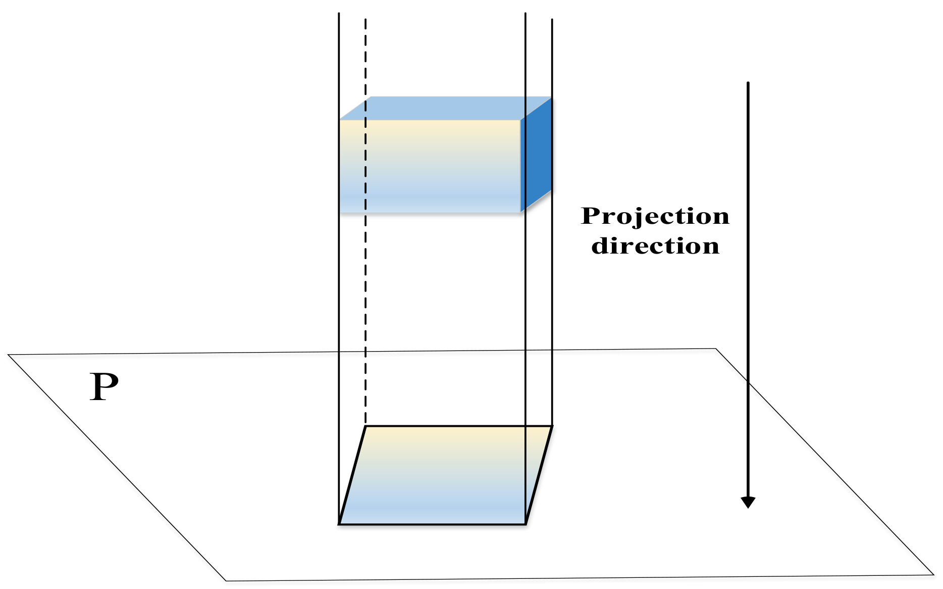
- The core problem is abstractly likened to a path planning problem with multiple starting points/endpoints, that is, the airspace projection projected onto a two-dimensional plane is approximately regarded as a ground obstacle. Using the Multi A * algorithm, by setting a relatively reasonable starting point and endpoint for many times, multiple clustering lines without contact and conflict with the obstacle (task airspace) can be planned. These clustering lines combine to divide the entire task area into multiple airspace clusters.
- (2)
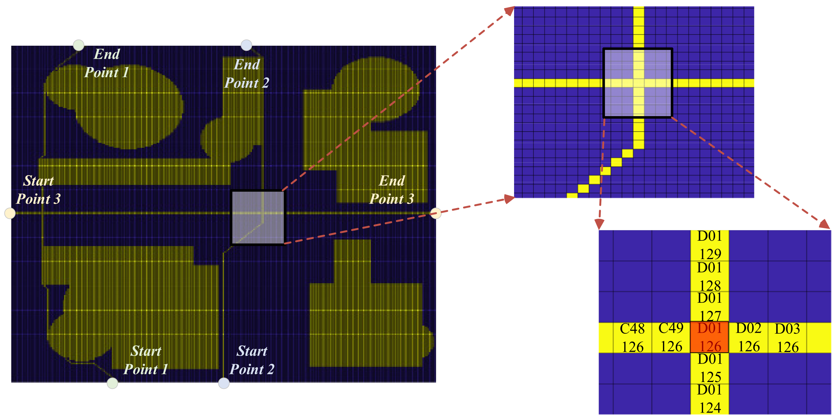
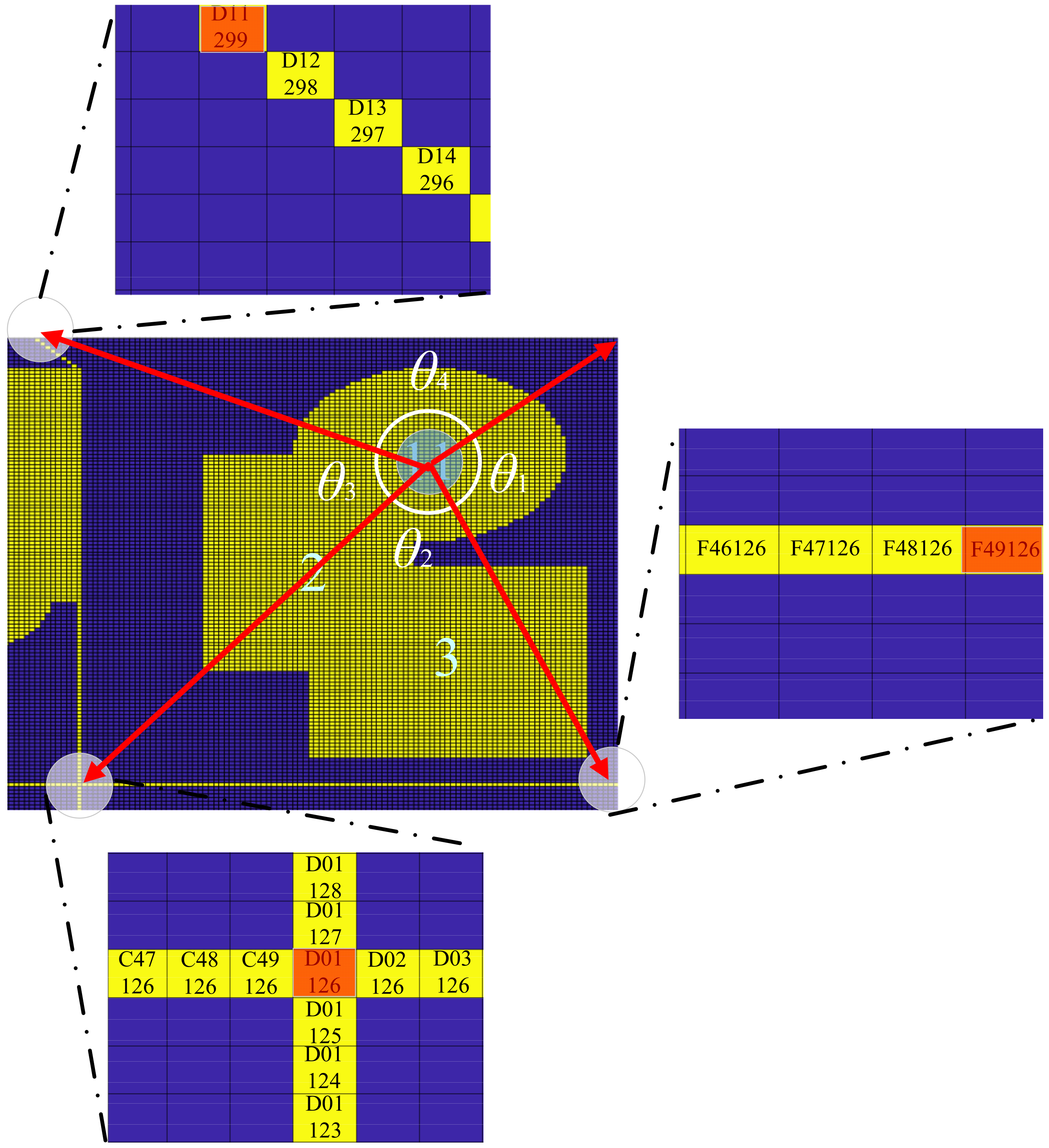
- On the basis of the first step, the airspace objects and path data are coded using the grid system, and the path-path intersection points (i.e., the vertices of each airspace cluster) are calculated through grid coding.
- (3)
- Finally, the number of the cluster where the center of the airspace is located is judged by “Angle Addition”, and the airspace clustering result is finally obtained.
3. Introduction to Theoretical Basis
4. Airspace Clustering Steps Based on Multi-A * Algorithm
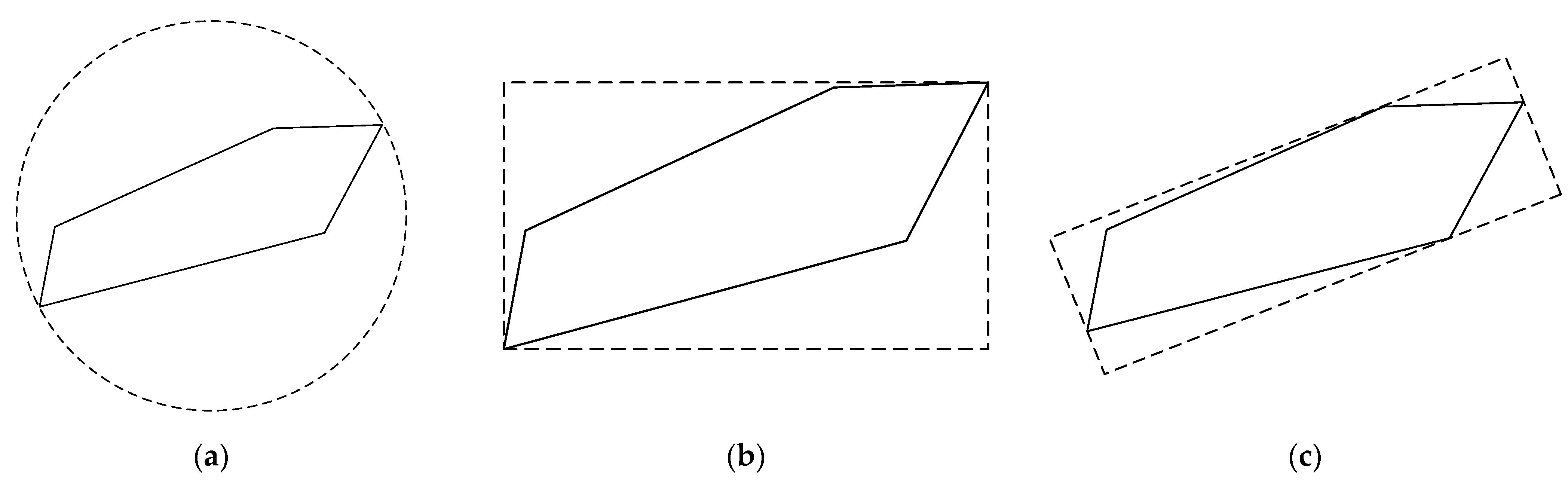
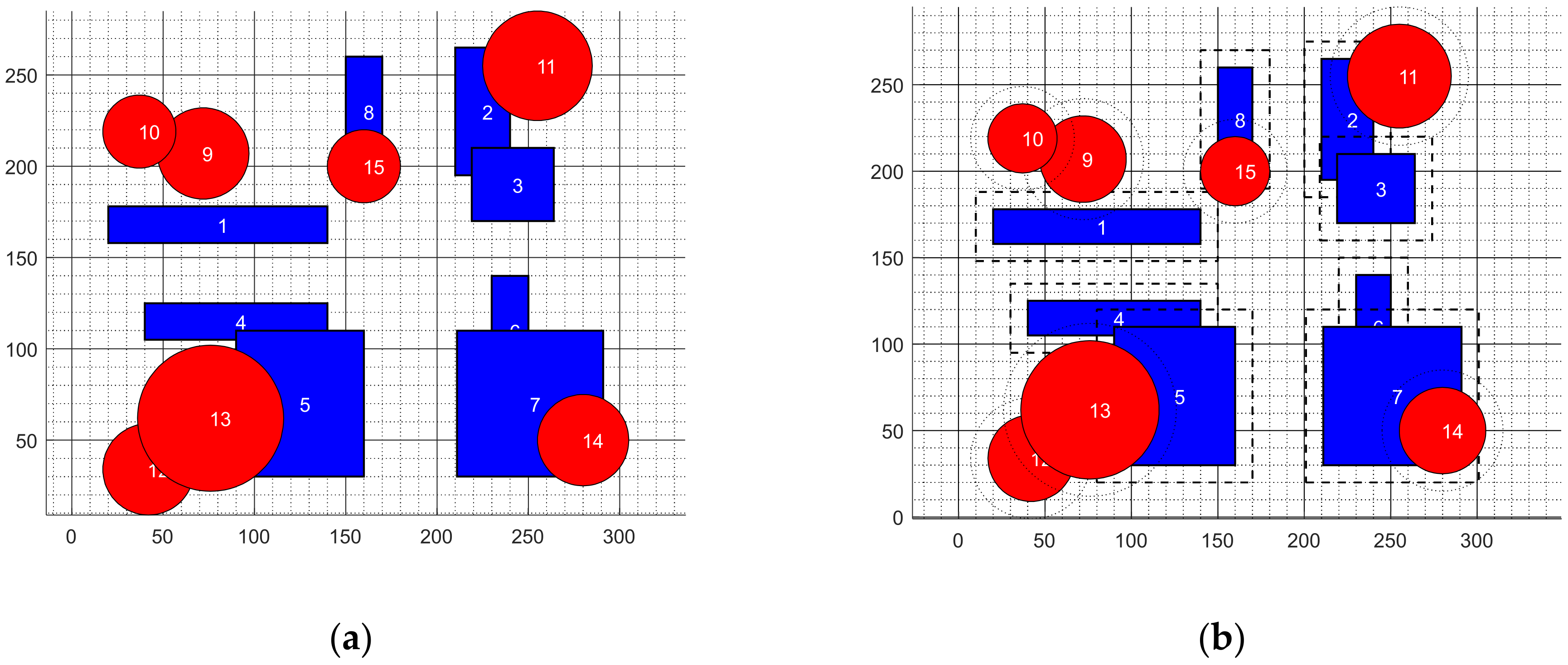
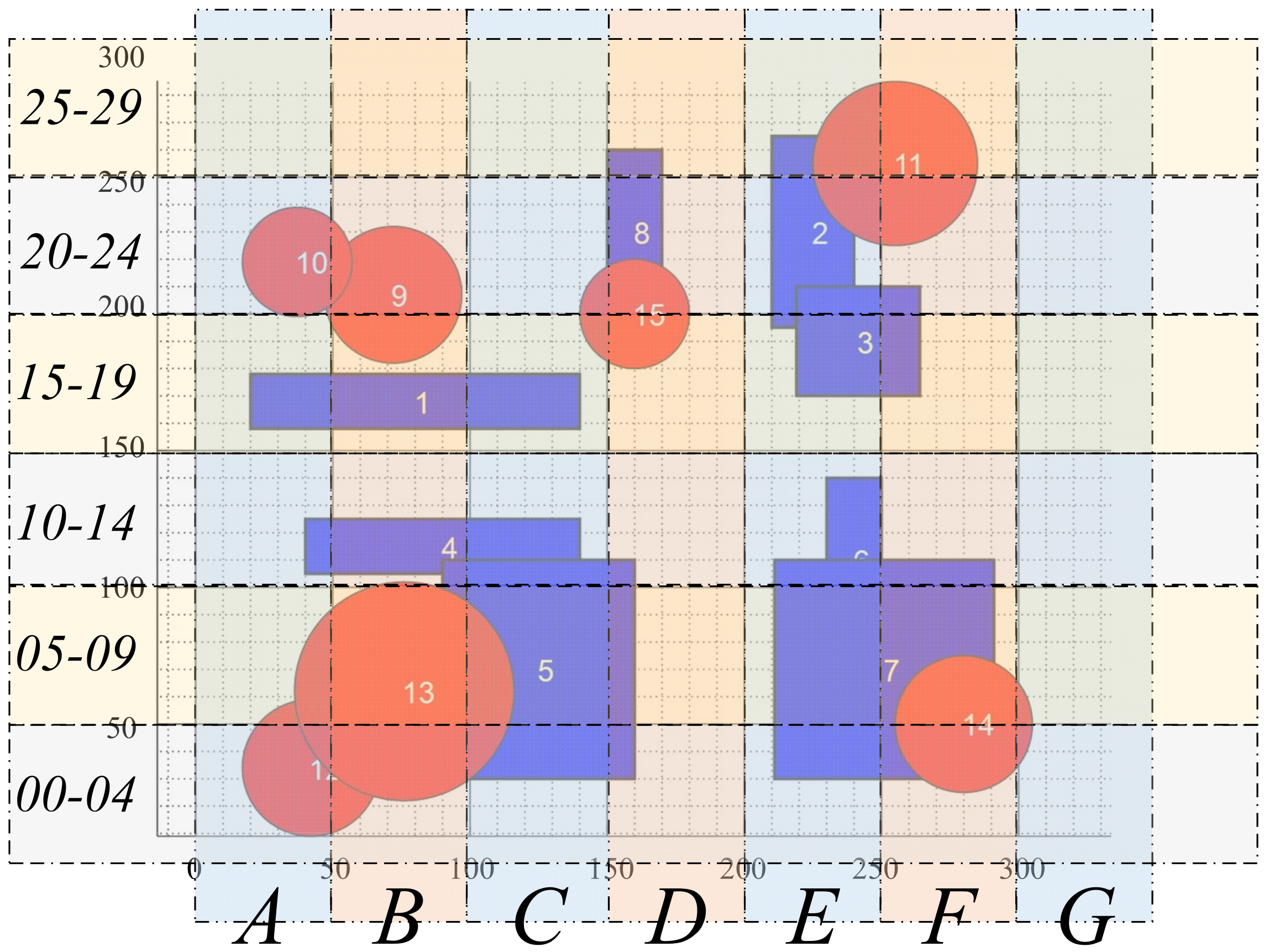
4.1. Construct Airspace Security Bounding Box
- (1)
- Simplicity: The bounding box itself should be a simple geometric figure relative to the surrounded polygons. In addition, the intersection test of the bounding box should be relatively simple, otherwise it will affect the efficiency.
- (2)
- Tightness: The bounding box should be as close to the polygon as possible, and closely enclose the polygon.
4.2. Airspace Projection Image Preprocessing
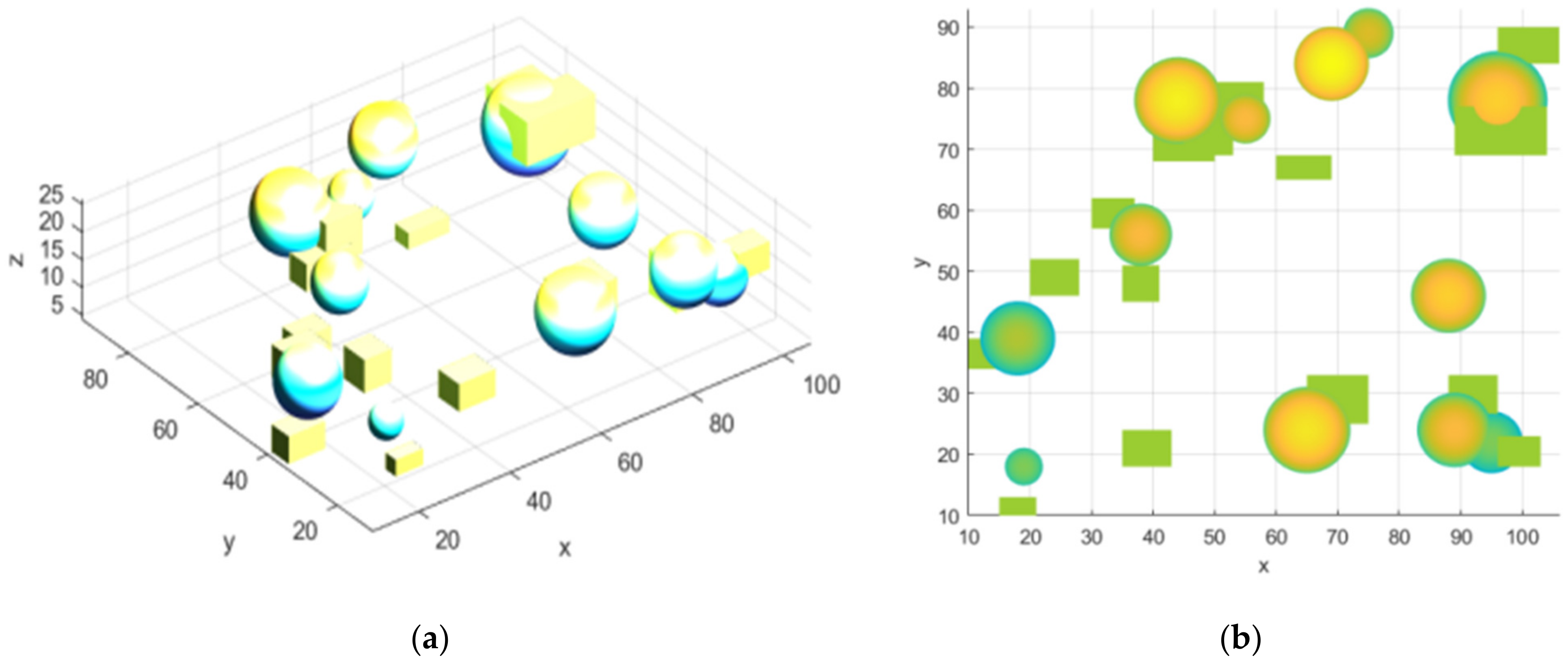
4.2.1. Mission Airspace Projection
4.2.2. Projection Image Processing
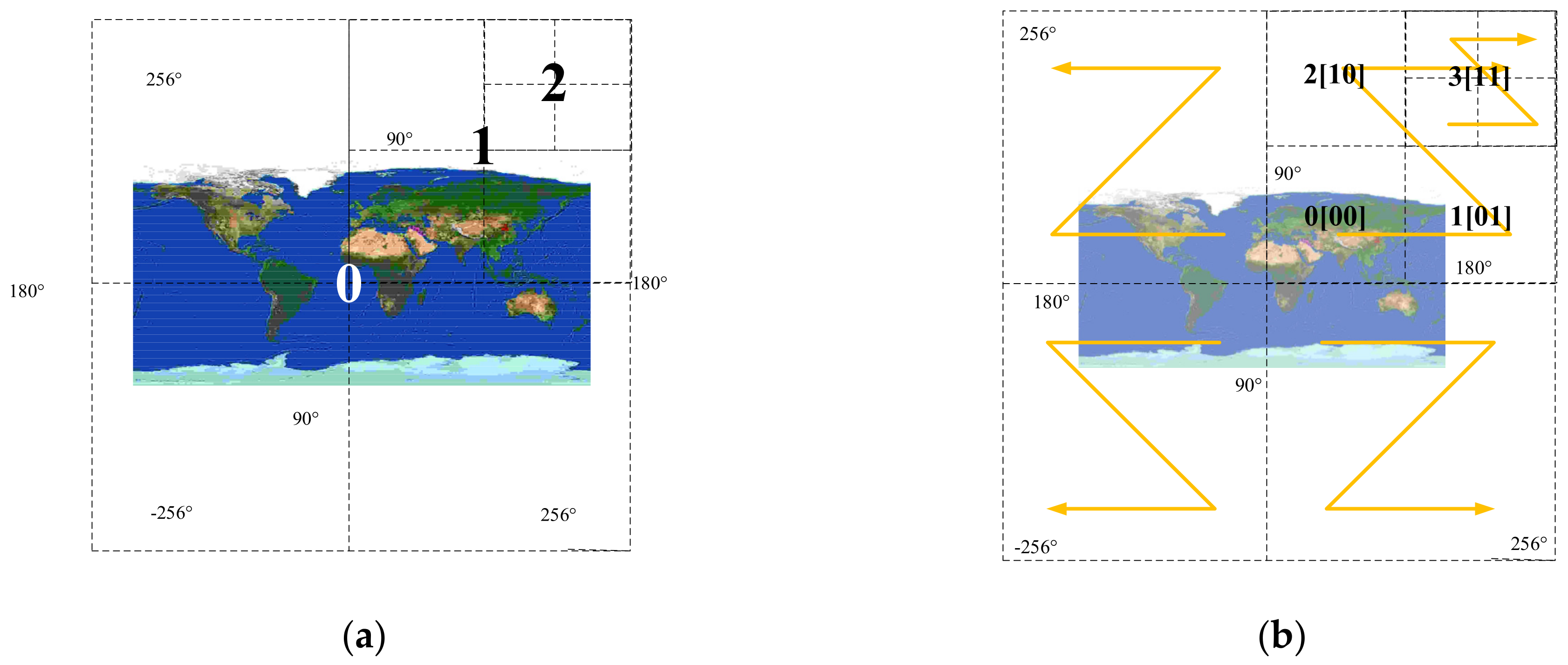
4.2.3. Grid Representation of Projected Image
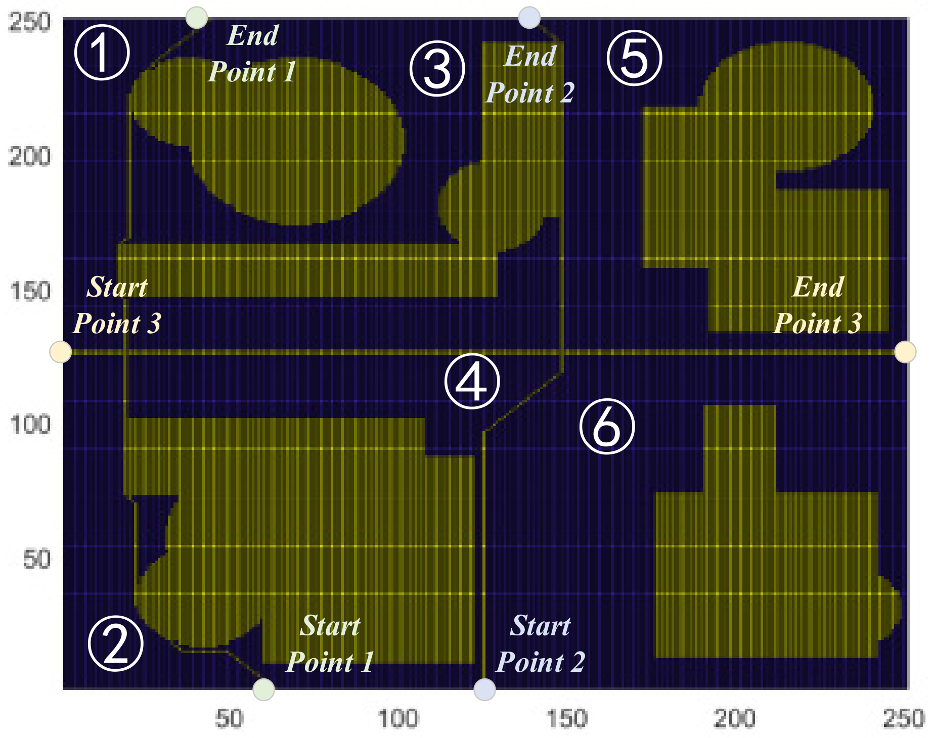
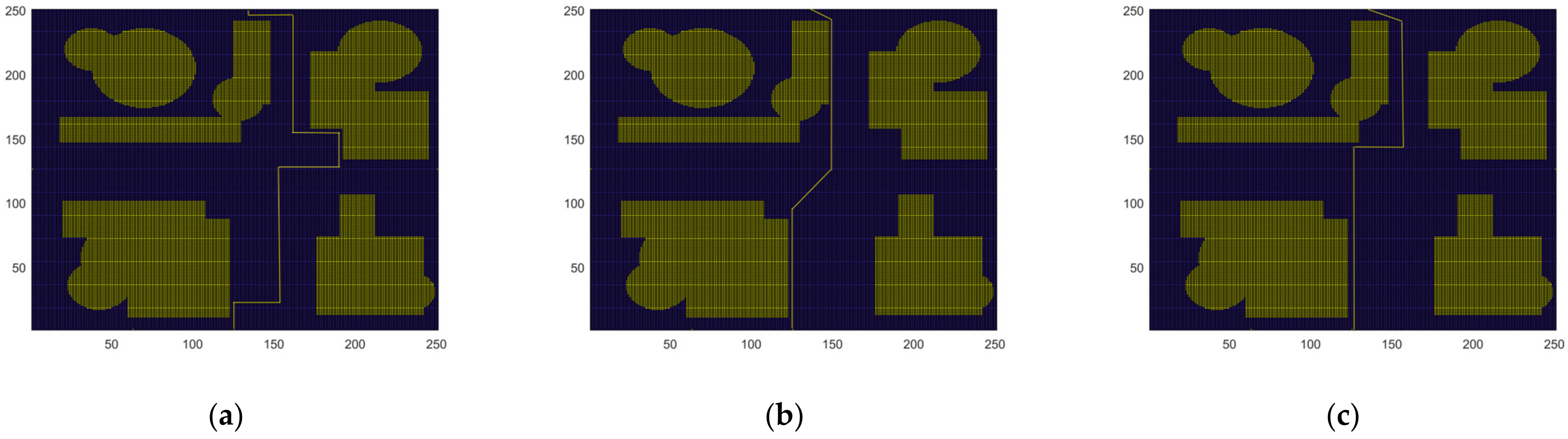
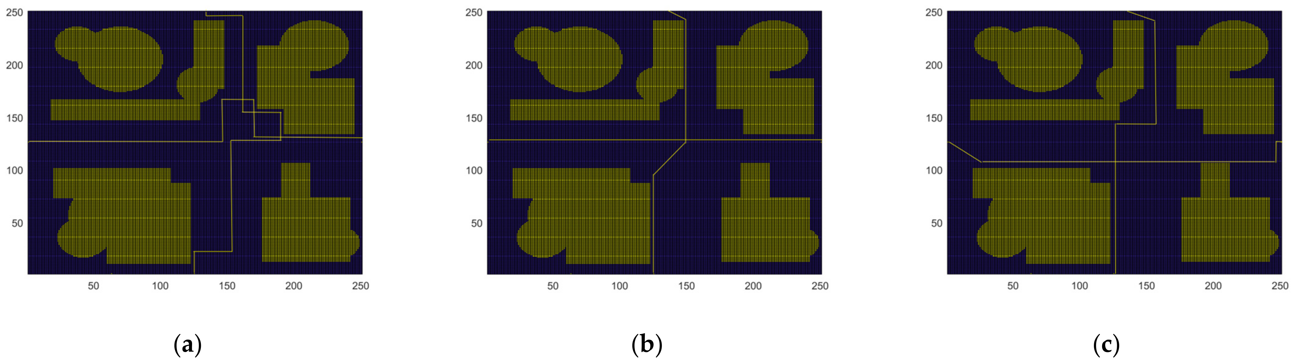
4.3. Using Multi A * Algorithm to Generate Edge Cluster Lines
4.4. Clustering Data Processing
4.4.1. Airspace Clustering Line Marking
4.4.2. Internal Element Identification of Airspace Cluster
5. Experimental Simulation and Analysis
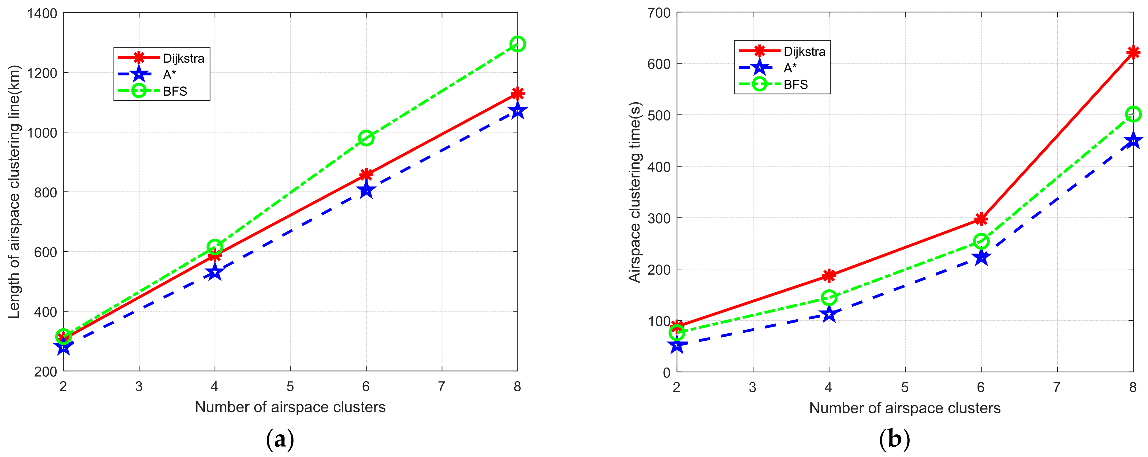
5.1. Algorithm Comparison Experiment
5.2. Evaluation of Airspace Clustering Effect
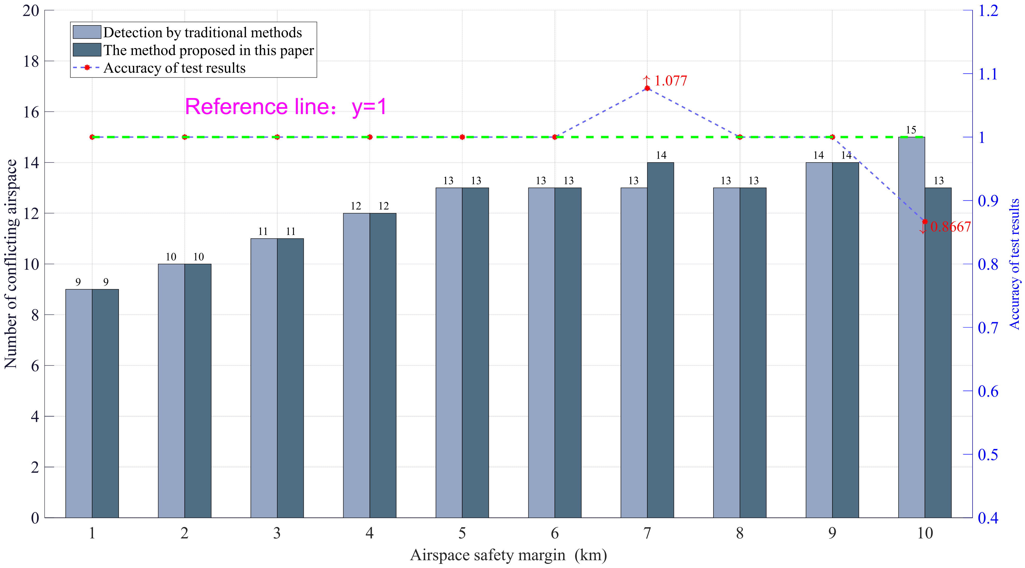
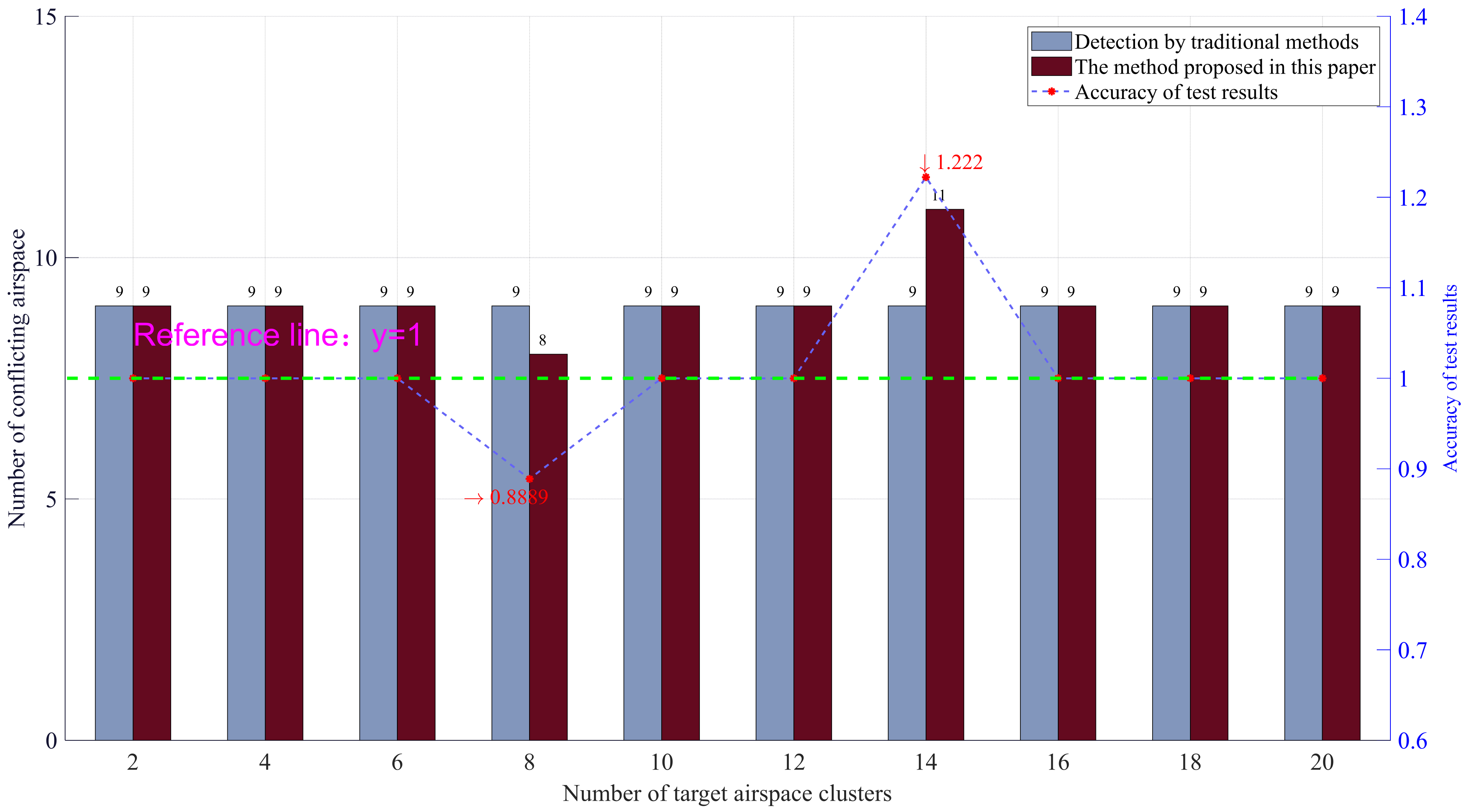
5.2.1. Definition of Experimental Index Operator
- (1)
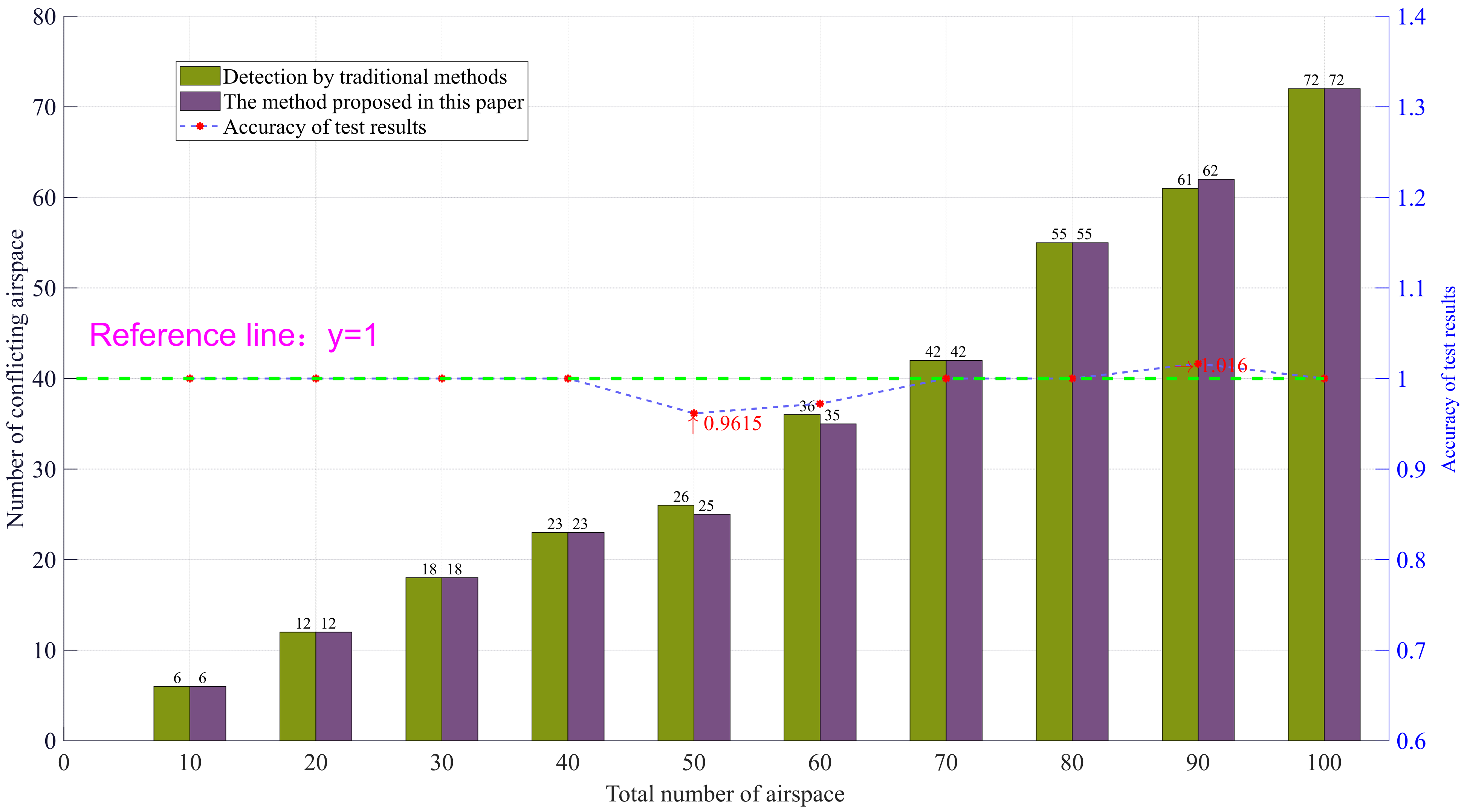
- Detection accuracy
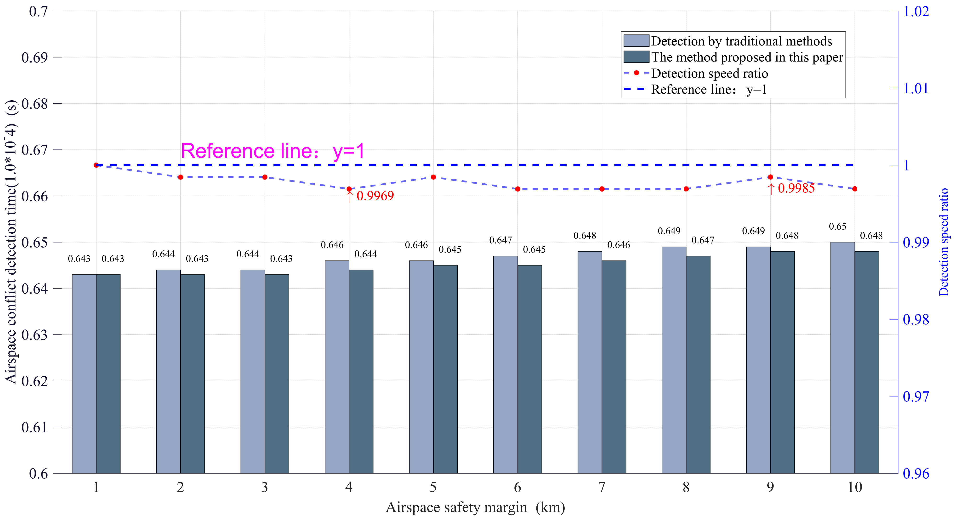
- (2)
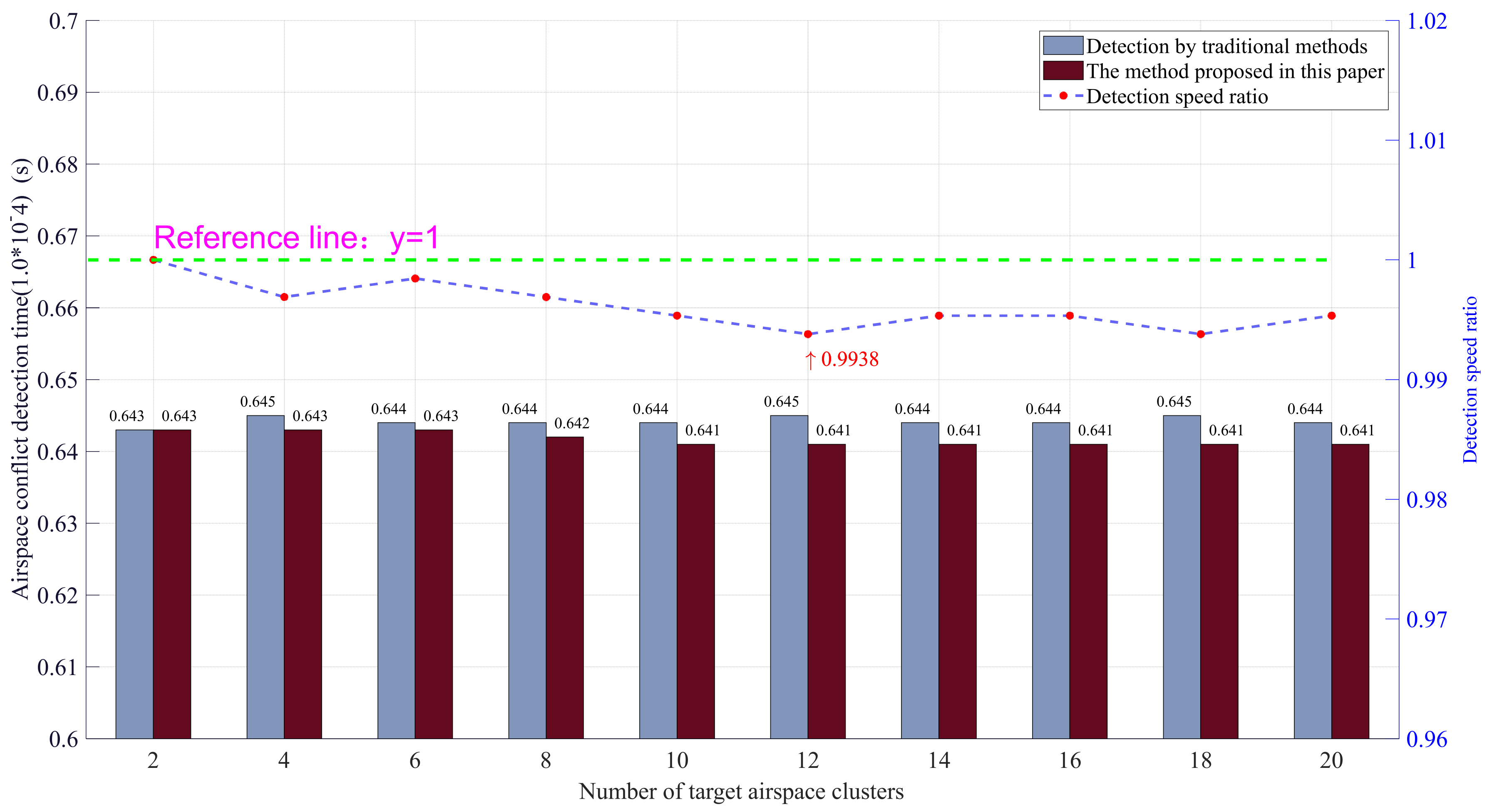
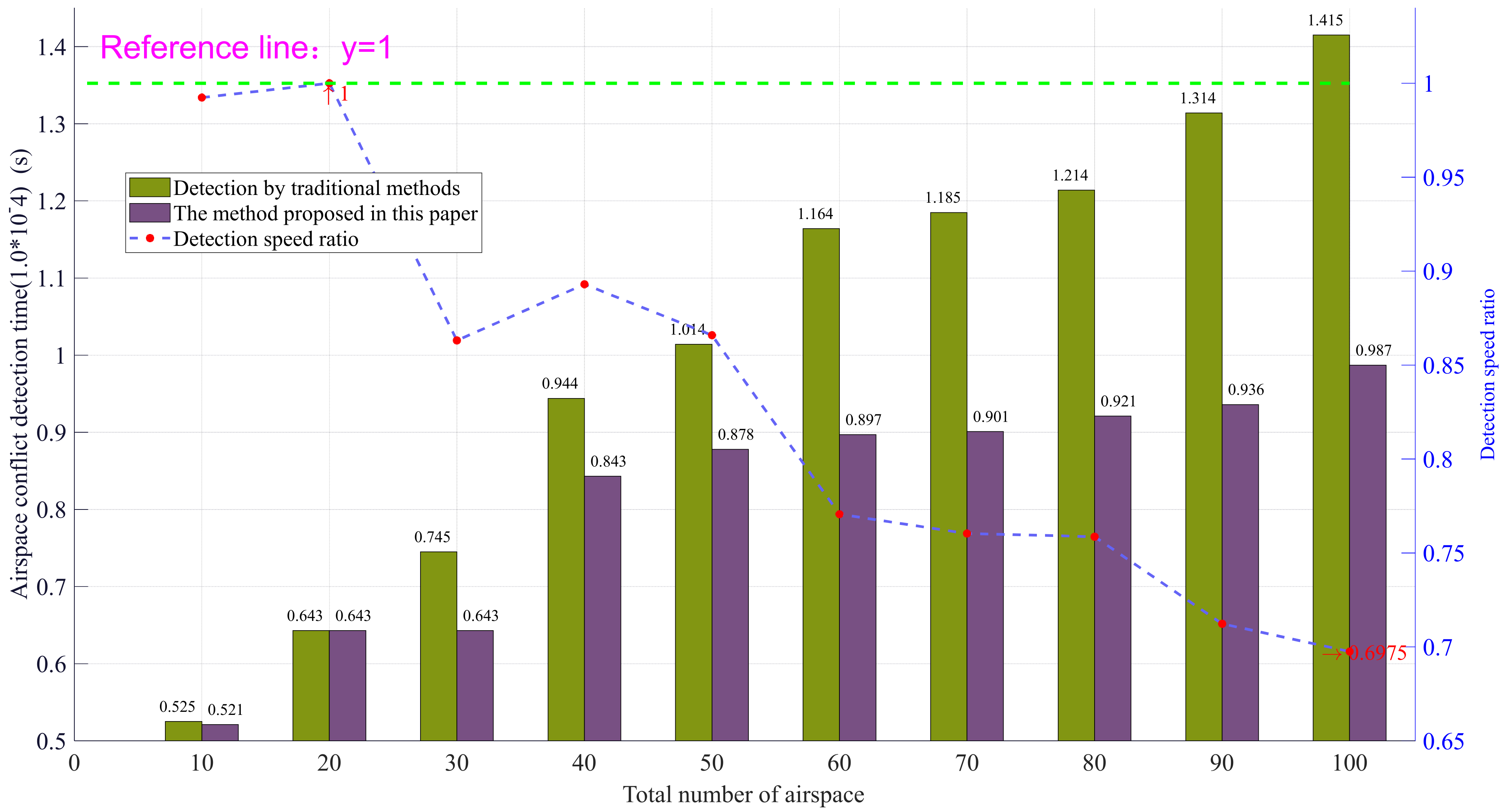
- Detection speed ratio
5.2.2. Experimental Results and Analysis
6. Conclusions
- (1)
- The accuracy of detection results of airspace conflict detection based on airspace clustering is different from that of traditional wide area airspace conflict detection. The main reason is that there are some fuzzy disputes near the edge cluster lines in the airspace, which may lead to multiple or missing detections in the overall detection due to unclear clustering results, and ultimately affect the accuracy of detection.
- (2)
- Although there are differences in the accuracy of detection results between airspace conflict detection based on airspace clustering and traditional airspace conflict detection based on wide area, this difference can be continuously reduced by adjusting the number of airspace and other parameters, especially in the case of large-scale task airspace, the accuracy of the method proposed in this paper has been gradually improved, and the error rate is also declining.
- (3)
- Clustering the whole task airspace can effectively improve the efficiency of conflict detection. The larger the number and scale of airspace, the more time saved and the greater the speed difference between airspace conflict detection based on airspace clustering and traditional detection methods. This shows that airspace clustering is a pre preparation work when facing the challenge of large-scale airspace tasks. It has great application potential and great significance.
- (4)
- The efficiency of airspace conflict detection based on airspace clustering mentioned in point (3) is restricted by many factors. For example, when the number of airspace is limited, simply increasing the number of airspace clusters will lead to the saturation of airspace clustering, and the detection efficiency will gradually decrease. Therefore, the number of battlefield airspace and other parameters should be sorted, integrated, analyzed, and calculated in advance before airspace clustering, in this way, reasonable airspace clustering can be carried out to achieve the best operational efficiency.
- (5)
- The method proposed in this paper provides a new idea for the traditional battlefield airspace management. Such a simplified dimension reduction method greatly improves the accuracy of battlefield airspace management and also greatly releases the burden and pressure of battlefield airspace management and control. It is expected to be applied to large-scale joint operations in the future and become the key and booster of efficient and safe battlefield airspace management and control.
Author Contributions
Funding
Data Availability Statement
Acknowledgments
Conflicts of Interest
References
- Zhang, W.L.; Jiang, H. On the concept of airspace. J. Beijing Univ. Aeronaut. Astronaut. (Soc. Sci. Ed.) 2021, 34, 127–133. [Google Scholar]
- Zhu, Y.J. Study on the Process of European Airspace Integration. Master’s Thesis, Fudan University, Shanghai, China, 2013. [Google Scholar]
- ICAO DOC 8168; Procedures for Air Navigation Services: Aircraft Operations. ICAO: Montreal, QC, Canada, 2006.
- Thipphavong, D.P.; Apaza, R.; Barmore, B.; Battiste, V.; Burian, B.; Dao, Q.; Feary, M.; Go, S.; Goodrich, K.H.; Homola, J. Urban air mobility airspace integration concepts and considerations. In Proceedings of the 2018 Aviation Technology, Integration, and Operations Conference, Atlanta, Georgia, 25–29 June 2018; p. 3676. [Google Scholar]
- Air Land Sea Application Center. Army Airspace Management during Large-Scale Combat Operations. Available online: https://www.alsa.mil/Portals/9/Documents/articles/220501_ALSA_Article_Cronen_Airspace.pdf (accessed on 1 May 2022).
- Gerdes, I.; Temme, A.; Schultz, M. Dynamic airspace sectorisation for flight-centric operations. Transp. Res. Part C Emerg. Technol. 2018, 95, 460–480. [Google Scholar] [CrossRef]
- Vascik, P.D.; Cho, J.; Bulusu, V.; Polishchuk, V. Geometric approach towards airspace assessment for emerging operations. J. Air Transp. 2020, 28, 124–133. [Google Scholar] [CrossRef]
- Yang, B.; Wang, B.; Feng, C. Research on the General Framework of Army Tactical Airspace Command and Control System. pp. 127–131. Available online: https://cpfd.cnki.com.cn/Article/CPFDTOTAL-ZHKZ201507002029.htm (accessed on 7 July 2015).
- Zheng, L.H.; Tao, J.D. Software Technology of Land Tactical Airspace Management and Control System. Command Inf. Syst. Technol. 2020, 11, 1–4. [Google Scholar]
- Hang, W.N.; Wu, H.X. U.S. High-Altitude E-Class Airspace Management (ETM) Operation Concept. pp. 528–541. Available online: https://kns.cnki.net/kcms/detail/detail.aspx?dbcode=CPFD&dbname=CPFDLAST2022&filename=ZGHU202111001094&uniplatform=NZKPT&v=JGihuccHY0POIfy4DtAdL1dL55x0-drLCQMAAyyixbqm2T34WtByUUfjZhWUgrVMB_91WC0q3GQ%3d (accessed on 9 November 2021).
- Xun, C.C.; Liu, G.B.; Zhao, X.L.; Ding, Y. American Air Battlefield Management and Control Information System. pp. 156–161. Available online: https://kns.cnki.net/kcms/detail/detail.aspx?dbcode=CPFD&dbname=CPFDLAST2021&filename=ZHKZ202107001028&uniplatform=NZKPT&v=HvtzC_hzgnVIBZspQsqvAYlxWd2cqz668Tz4mxi8tRCWQtWjbKxeqiu-EWGzRe8wya1NNeA4e68%3d (accessed on 5 July 2021).
- Fang, F.; Zhu, X.Y.; Zhang, Z.Z. Research on Airspace Management System of US Army Land Battlefield. Firepower Command Control. 2017, 42, 170–173. [Google Scholar]
- Xue, M. Airspace sector redesign based on Voronoi diagrams. J. Aerosp. Comput. Inf. Commun. 2009, 6, 624–634. [Google Scholar] [CrossRef]
- Sabhnani, G.; Yousefi, A.; Mitchell, J.S. Flow conforming operational airspace sector design. In Proceedings of the 10th AIAA Aviation Technology, Integration, and Operations (ATIO) Conference, Fort Worth, TX, USA, 13–15 September 2010; p. 9377. [Google Scholar]
- Zhang, M.; Shan, L.; Liu, K.; Yu, H.; Yu, J. Terminal airspace sector capacity estimation method based on the ATC dynamical model. Kybernetes 2016, 45, 884–899. [Google Scholar] [CrossRef]
- Lv, H.L. Sector Combination Optimization Based on Flexible Use of Airspace Concept. Master’s Thesis, China Civil Aviation Flight Academy, Sichuan, China, 2014. [Google Scholar]
- Feng, D.; Zeng, L.; Wang, F.; Liu, D.; Zhang, F.; Qin, L.; Liu, Q. Geographic Information Systems Grid. pp. 823–830. Available online: https://link.springer.com/chapter/10.1007/11508380_84 (accessed on 29 May 2021).
- Yan, J.; Chengqi, C.; Beitong, Z.; Weixin, Z. Geographic Airspace Semantic Translation Method Using Subdivision Grid Coding. pp. 4534–4537. Available online: https://ieeexplore.ieee.org/document/7326836 (accessed on 15 December 2020).
- Ware, C.; Mayer, L.; Johnson, P.; Jakobsson, M.; Ferrini, V. A global geographic grid system for visualizing bathymetry. Geosci. Instrum. Methods Data Syst. 2020, 9, 375–384. [Google Scholar] [CrossRef]
- Wang, S.; Armstrong, M.P. A quadtree approach to domain decomposition for airspace interpolation in grid computing environments. Parallel Comput. 2003, 29, 1481–1504. [Google Scholar] [CrossRef]
- AlShawi, I.S.; Yan, L.; Pan, W.; Luo, B. Lifetime enhancement in wireless sensor networks using fuzzy approach and A-star algorithm. IEEE Sens. J. 2012, 12, 3010–3018. [Google Scholar] [CrossRef]
- Zhang, Z.; Zhao, Z. A multiple mobile robots path planning algorithm based on A-star and Dijkstra algorithm. Int. J. Smart Home 2014, 8, 75–86. [Google Scholar] [CrossRef] [Green Version]
- Yao, J.; Lin, C.; Xie, X.; Wang, A.J.; Hung, C.C. Path planning for virtual human motion using improved A* star algorithm. In Proceedings of the 2010 Seventh International Conference on Information Technology: New Generations, Las Vegas, NV, USA, 12–14 April 2010; pp. 1154–1158. [Google Scholar]
- Duchoň, F.; Babinec, A.; Kajan, M.; Beňo, P.; Florek, M.; Fico, T.; Jurišica, L. Path planning with modified a star algorithm for a mobile robot. Procedia Eng. 2014, 96, 59–69. [Google Scholar] [CrossRef] [Green Version]
- Liu, Z.; Nan, Y.; Yang, Y. Airspace Conflict Detection Method Based on Subdivision Grid. Artif. Intell. China 2022, 854, 670–677. [Google Scholar]
- Zhao, H.; Zhang, Y.Q.; Fan, Q.; Wang, W.C. Coordinate transformation of geographic information data based on grid model. Surv. Mapp. Airsp. Geogr. Inf. 2022, 43, 201–203, 207, 211. [Google Scholar]
- Jin, A.; Chen, C.Q. airspace data coding method based on global grid. J. Surv. Mapp. Sci. Technol. 2013, 30, 284–287. [Google Scholar]
- Li, Z.Q.; Chen, C.Q.; Li, S. Fast Visualization and Experimental Analysis of airspace Objects Based on GeoSOT-3D. J. Earth Inf. Sci. 2015, 17, 810–815. [Google Scholar]
- Xu, X.Y.; Wan, L.J.; Chen, P.; Dai, J.B.; Cai, M. Airspace Rasterization Representation Method Based on GeoSOT Grid. J. Air Force Eng. Univ. (Nat. Sci. Ed.) 2021, 22, 15–22. [Google Scholar]
- Chen, C.Q.; Wu, F.L.; Wang, R.; Qin, Y.G.; Tong, X.C.; Chen, B. Preliminary study on the construction of geoairspace reference grid system. J. Peking Univ. (Nat. Sci. Ed.) 2016, 52, 1041–1049. [Google Scholar]
- Wang, L.; Wu, W.; Deng, G.Q.; Tong, X.C.; Li, J.F. Analysis of Geoairspace Grid Coding Technology. Bull. Surv. Mapp. 2020, 10, 131–134, 147. [Google Scholar]
- Russ, J.C. The Image Processing Handbook; CRC Press: Boca Raton, FL, USA, 2006. [Google Scholar]
- Acharya, T.; Ray, A.K. Image Processing: Principles and Applications; John Wiley & Sons: Hoboken, NJ, USA, 2005. [Google Scholar]
- Haralick, R.M.; Shapiro, L.G. Image segmentation techniques. Comput. Vis. Graph. Image Process. 1985, 29, 100–132. [Google Scholar] [CrossRef]
- Heel, M.V.; Harauz, G.; Orlova, E.V.; Schmidt, R.; Schatz, M. A new generation of the IMAGIC image processing system. J. Struct. Biol. 1996, 116, 17–24. [Google Scholar] [CrossRef] [Green Version]
- Zhu, S.; Xia, X.; Zhang, Q.; Belloulata, K. An image segmentation algorithm in image processing based on threshold segmentation. In Proceedings of the 2007 Third International IEEE Conference on Signal-Image Technologies and Internet-Based System, Shanghai, China, 16–18 December 2007; pp. 673–678. [Google Scholar]
- Al-Amri, S.S.; Kalyankar, N.V. Image segmentation by using threshold techniques. arXiv 2010, arXiv:1005.4020. [Google Scholar]
- Cuevas, E.; Zaldivar, D.; Pérez-Cisneros, M. A novel multi-threshold segmentation approach based on differential evolution optimization. Expert Syst. Appl. 2010, 37, 5265–5271. [Google Scholar] [CrossRef]
- Bhargavi, K.; Jyothi, S. A survey on threshold based segmentation technique in image processing. Int. J. Innov. Res. Dev. 2014, 3, 234–239. [Google Scholar]
- Huang, Y.C.; Tung, Y.S.; Chen, J.C.; Wang, S.W.; Wu, J.L. An adaptive edge detection based colorization algorithm and its applications. In Proceedings of the 13th annual ACM international conference on Multimedia, Beijing, China, 6–11 November 2005; pp. 351–354. [Google Scholar]
- Salman, N.; Liu, C.Q. Image segmentation and edge detection based on watershed techniques. Int. J. Comput. Appl. 2003, 25, 258–263. [Google Scholar] [CrossRef]
- Bogovic, J.A.; Prince, J.L.; Bazin, P.L. A multiple object geometric deformable model for image segmentation. Comput. Vis. Image Underst. 2013, 117, 145–157. [Google Scholar] [CrossRef] [Green Version]
- Wong, W.E.; Debroy, V.; Gao, R.; Li, Y. The DStar method for effective software fault localization. IEEE Trans. Reliab. 2013, 63, 290–308. [Google Scholar] [CrossRef]
- Li, B.; Chen, B. An adaptive rapidly-exploring random tree. IEEE/CAA J. Autom. Sin. 2021, 9, 283–294. [Google Scholar] [CrossRef]
- Zhu, Y.W.; Chen, Z.J.; Pu, F.; Wang, J.L. Research on the Development of Digital Airspace System. China Eng. Sci. 2021, 23, 135–143. [Google Scholar] [CrossRef]
- Zhu, Y.W.; Xie, H.; Pu, F.; Zhang, Y.; He, W.W. Research on airspace grid method and its application in ATC. Prog. Aeronaut. Eng. 2021, 12, 12–24. [Google Scholar]
- Zhu, Y.W.; Pu, F. Principle and Application of airspace Grid Identification in Airspace. J. Beijing Univ. Aeronaut. Astronaut. 2021, 47, 2462–2474. [Google Scholar]
- Kicinger, R.; Yousefi, A. Heuristic method for 3D airspace partitioning: Genetic algorithm and agent-based approach. In Proceedings of the 9th AIAA Aviation Technology, Integration, and Operations Conference (ATIO), Hilton Head, SC, USA, 21–23 September 2009; p. 7058. [Google Scholar]
- Zheng, Y.; Liu, J.; Li, J.; Xu, Y.; Huang, Q.; Zhu, Y.; Pei, Y. Design of Fine Management System for Civil Aviation Airspace Resources Based on Spatiotemporal Grid Model. In Proceedings of the 2019 IEEE 1st International Conference on Civil Aviation Safety and Information Technology (ICCASIT), Kunming, China, 17–19 October 2019; pp. 547–551. [Google Scholar]
- Sun, G.; Qu, T.; Han, B.; Sun, H.; Zhang, Q. Research on Airspace Grid Modeling Based on GeoSOT Global Subdivision Model. In Proceedings of the 2021 IEEE 3rd International Conference on Civil Aviation Safety and Information Technology (ICCASIT), Changsha, China, 20–22 October 2021; pp. 501–505. [Google Scholar]
- Qian, C.; Yi, C.; Cheng, C.; Pu, G.; Wei, X.; Zhang, H. Geosot-based spatiotemporal index of massive trajectory data. ISPRS Int. J. Geo-Inf. 2019, 8, 284. [Google Scholar] [CrossRef] [Green Version]
- Lu, N.; Cheng, C.; Jin, A.; Ma, H. An index and retrieval method of airspace data based on GeoSOT global discrete grid system. In Proceedings of the 2013 IEEE International Geoscience and Remote Sensing Symposium—IGARSS, Melbourne, VIC, Australia, 21–26 July 2013; pp. 4519–4522. [Google Scholar]
- Hou, K.; Cheng, C.; Chen, B.; Zhang, C.; He, L.; Meng, L.; Li, S. A set of integral grid-coding algebraic operations based on geosot-3d. ISPRS Int. J. Geo-Inf. 2021, 10, 489. [Google Scholar] [CrossRef]
- Song, S.H.; Chen, C.Q.; Pu, G.L.; An, F.G.; Luo, X. GeoSOT grid application of global remote sensing data subdivision organization. J. Surv. Mapp. 2014, 43, 869. [Google Scholar]
- Shu, P.; Zheng, Y.; Shi, H.; Liu, S.; Sun, H.; Zhou, X. Three dimensional grid model of airspace resources based on Beidou grid code. In Proceedings of the 2021 IEEE 3rd International Conference on Civil Aviation Safety and Information Technology (ICCASIT), Changsha, China, 20–22 October 2021; pp. 380–383. [Google Scholar]
- Shi, H.F.; Wang, Z.Y.; Zhen, Y.E.; Xu, Y.B. Fine management system of airspace resources based on Beidou grid code. J. Civ. Aviat. 2022, 6, 44–47. [Google Scholar]
- Delahaye, D.; Schoenauer, M.; Alliot, J.M. Airspace sectoring by evolutionary computation. In Proceedings of the 1998 IEEE International Conference on Evolutionary Computation Proceedings. IEEE World Congress on Computational Intelligence (Cat. No.98TH8360), Anchorage, AK, USA, 4–9 May 1998; pp. 218–223. [Google Scholar]
- Delahaye, D.; Puechmorel, S. 3D airspace sectoring by evolutionary computation: Real-world applications. In Proceedings of the 8th Annual Conference on Genetic and Evolutionary Computation, Washington, DC, USA, 27 October 2014; pp. 1637–1644. [Google Scholar]
- Klein, A. An efficient method for airspace analysis and partitioning based on equalized traffic mass. In Proceedings of the 6th USA/Europe Air Traffic Management R & D Seminar; George MasonUniversity: George, VA, USA, 2005. [Google Scholar]
- Trandac, H.; Baptiste, P.; Duong, V. Airspace sectorization with constraints. RAIRO-Oper. Res. 2005, 39, 105–122. [Google Scholar] [CrossRef]
- Granberg, T.A.; Polishchuk, T.; Polishchuk, V.; Schmidt, C. A framework for integrated terminal airspace design. Aeronaut. J. 2019, 123, 567–585. [Google Scholar] [CrossRef]
- Yousefi, A.; Donohue, G. Temporal and airspace distribution of airspace complexity for air traffic controller workload-based sectorization. In Proceedings of the AIAA 4th Aviation Technology, Integration and Operations (ATIO) Forum, Chicago, IL, USA, 20–22 September 2004; p. 6455. [Google Scholar]
- Delahaye, D.; Alliot, J.M.; Schoenauer, M.; Farges, J.L. Genetic algorithms for partitioning air space. In Proceedings of the Tenth Conference on Artificial Intelligence for Applications, San Antonio, TX, USA, 1–4 March 1994; pp. 291–297. [Google Scholar]
- Prandini, M.; Piroddi, L.; Puechmorel, S.; Brazdilova, S.L. Toward air traffic complexity assessment in new generation air traffic management systems. IEEE Trans. Intell. Transp. Syst. 2011, 12, 809–818. [Google Scholar] [CrossRef]
- Brinton, C.; Hinkey, J.; Leiden, K. Airspace sectorization by dynamic density. In Proceedings of the 9th AIAA Aviation Technology, Integration, and Operations Conference (ATIO), Hilton Head, CA, USA, 21–23 September 2009; p. 7102. [Google Scholar]
- Lee, K.; Feron, E.; Pritchett, A. Describing airspace complexity: Airspace response to disturbances. J. Guid. Control Dyn. 2009, 32, 210–222. [Google Scholar] [CrossRef]
- Sergeeva, M.; Delahaye, D.; Mancel, C. 3D airspace sector design by genetic algorithm. In Proceedings of the 2015 International Conference on Models and Technologies for Intelligent Transportation Systems (MT-ITS), Budapest, Hungary, 3–5 June 2015; pp. 499–506. [Google Scholar]
- Yu, D.; Ji, S. Grid based spherical cnn for object detection from panoramic images. Sensors 2019, 19, 2622. [Google Scholar] [CrossRef] [Green Version]
- Cai, P.; Indhumathi, C.; Cai, Y.; Zheng, J.; Gong, Y.; Lim, T.S.; Wong, P. Collision detection using axis aligned bounding boxes. In Simulations, Serious Games and Their Applications; Springer: Singapore, 2014; pp. 1–14. [Google Scholar]
- Mahovsky, J.; Wyvill, B. Fast ray-axis aligned bounding box overlap tests with plucker coordinates. J. Graph. Tools 2004, 9, 35–46. [Google Scholar] [CrossRef]
- Gottschalk, S.A. Collision Queries Using Oriented Bounding Boxes; The University of North Carolina at Chapel Hill: Chapel Hill, NC, USA, 2000. [Google Scholar]
- Eberly, D. Dynamic Collision Detection Using Oriented Bounding Boxes; Geometric Tools. Inc.: Chapel Hill, NC, USA, 2002. [Google Scholar]
- Ding, S.; Mannan, M.; Poo, A.N. Oriented bounding box and octree based global interference detection in 5-axis machining of free-form surfaces. Comput.—Aided Des. 2004, 36, 1281–1294. [Google Scholar] [CrossRef]
- Havel, J.; Herout, A. Yet faster ray-triangle intersection (using SSE4). IEEE Trans. Vis. Comput. Graph. 2009, 16, 434–438. [Google Scholar] [CrossRef]
- Zhang, X.L.; Wang, S.; Hou, B.; Chan, C.T. Dynamically encircling exceptional points: In situ control of encircling loops and the role of the starting point. Phys. Rev. 2018, 8, 021066. [Google Scholar] [CrossRef] [Green Version]
- Cunningham, C.H.; Pauly, J.M.; Nayak, K.S. Saturated double-angle method for rapid B1+ mapping. Magn. Reson. Med. Off. J. Int. Soc. Magn. Reson. Med. 2006, 55, 1326–1333. [Google Scholar] [CrossRef]


| Grid Size | Grid Code |
|---|---|
| Airspace Number | Airspace Position | Airspace Shape | Airspace Size (km) | Usage Time | Communication Frequency |
|---|---|---|---|---|---|
| 1 | B316 | Rectangle | 120 × 20 | 8:00–10:00 | 87.975 MHz |
| 2 | E222 | Rectangle | 30 × 70 | 9:00–10:00 | 67.975 MHz |
| 3 | E418 | Rectangle | 45 × 40 | 7:00–8:00 | 77.975 MHz |
| 4 | B411 | Rectangle | 100 × 20 | 7:00–9:00 | 87.975 MHz |
| 5 | C206 | Rectangle | 70 × 80 | 8:00–10:00 | 87.975 MHz |
| 6 | E209 | Rectangle | 20 × 60 | 9:00–11:00 | 77.975 MHz |
| 7 | F006 | Rectangle | 80 × 80 | 14:00–16:00 | 67.975 MHz |
| 8 | D122 | Rectangle | 20 × 60 | 15:00–17:00 | 67.975 MHz |
| 9 | B221 | Circle | 25 | 7:00–10:00 | 87.975 MHz |
| 10 | A222 | Circle | 20 | 8:00–9:00 | 87.975 MHz |
| 11 | F025 | Circle | 30 | 9:00–10:00 | 77.975 MHz |
| 12 | A303 | Circle | 25 | 8:00–11:00 | 87.975 MHz |
| 13 | B206 | Circle | 40 | 15:00–16:00 | 67.975 MHz |
| 14 | F204 | Circle | 25 | 13:00–17:00 | 67.975 MHz |
| 15 | D119 | Circle | 20 | 16:00–18:00 | 87.975 MHz |
| Airspace Cluster Number | Airspace Number |
|---|---|
| ① | none |
| ② | none |
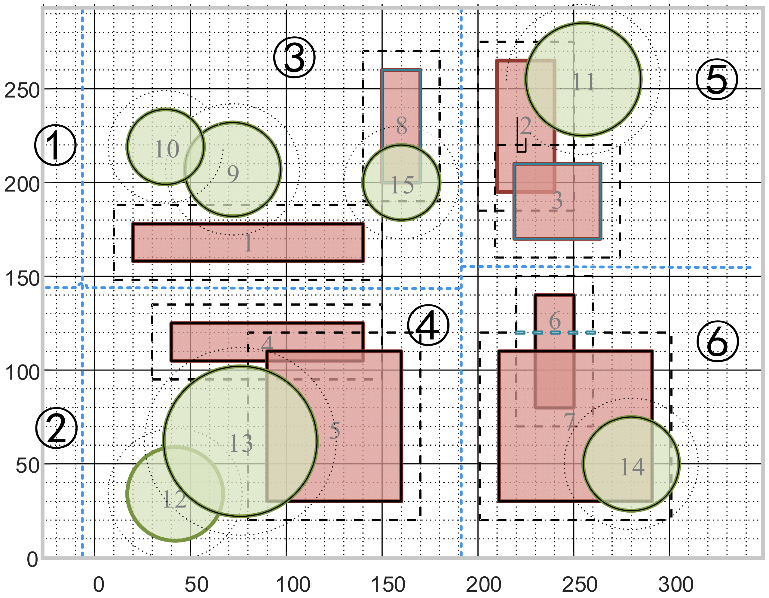
| ③ | 1, 8, 9, 10, 15 |
| ④ | 4, 5, 12, 13 |
| ⑤ | 2, 3, 11 |
| ⑥ | 6, 7, 14 |
| Serial Number | Variable Name | Variable Meaning | Data Type |
|---|---|---|---|
| 1 | Grid code | Unsigned Int | |
| 2 | The object grid coding set in the clustering line | BLOB | |
| 3 | The object grid coding set in the clustering line | BLOB |
| Number of Airspace Clusters | Algorithm Name | Length of Airspace Clustering Line (km) | Airspace Clustering Time (s) |
|---|---|---|---|
| 2 | Dijkstra | 307 | 88.19 |
| A * | 281 | 52.17 | |
| BFS | 315 | 76.32 | |
| 4 | Dijkstra | 587 | 187.25 |
| A * | 531 | 112.53 | |
| BFS | 615 | 144.36 | |
| 6 | Dijkstra | 857 | 297.23 |
| A * | 806 | 223.15 | |
| BFS | 980 | 254.13 | |
| 8 | Dijkstra | 1129 | 621.35 |
| A * | 1072 | 450.19 | |
| BFS | 1295 | 501.32 |
Publisher’s Note: MDPI stays neutral with regard to jurisdictional claims in published maps and institutional affiliations. |
© 2022 by the authors. Licensee MDPI, Basel, Switzerland. This article is an open access article distributed under the terms and conditions of the Creative Commons Attribution (CC BY) license (https://creativecommons.org/licenses/by/4.0/).
Share and Cite
Cai, M.; Wan, L.; Jiao, Z.; Lv, M.; Gao, Z.; Qi, D. Clustering Method of Large-Scale Battlefield Airspace Based on Multi A * in Airspace Grid System. Appl. Sci. 2022, 12, 11396. https://doi.org/10.3390/app122211396
Cai M, Wan L, Jiao Z, Lv M, Gao Z, Qi D. Clustering Method of Large-Scale Battlefield Airspace Based on Multi A * in Airspace Grid System. Applied Sciences. 2022; 12(22):11396. https://doi.org/10.3390/app122211396
Chicago/Turabian StyleCai, Ming, Lujun Wan, Zhiqiang Jiao, Maolong Lv, Zhizhou Gao, and Duo Qi. 2022. "Clustering Method of Large-Scale Battlefield Airspace Based on Multi A * in Airspace Grid System" Applied Sciences 12, no. 22: 11396. https://doi.org/10.3390/app122211396
APA StyleCai, M., Wan, L., Jiao, Z., Lv, M., Gao, Z., & Qi, D. (2022). Clustering Method of Large-Scale Battlefield Airspace Based on Multi A * in Airspace Grid System. Applied Sciences, 12(22), 11396. https://doi.org/10.3390/app122211396