Article

Self-Organized Fuzzy Neural Network Nonlinear System Modeling Method Based on Clustering Algorithm

College of Locomotive and Rolling Stock Engineering, Dalian Jiaotong University, Dalian 116028, China
*
Author to whom correspondence should be addressed.
Appl. Sci. 2022, 12(22), 11435; https://doi.org/10.3390/app122211435
Submission received: 9 October 2022 / Revised: 3 November 2022 / Accepted: 8 November 2022 / Published: 11 November 2022
(This article belongs to the Topic Advances in Artificial Neural Networks)

Abstract

:
In this paper, an improved self-organizing fuzzy neural network (SOFNN-CA) based on a clustering algorithm is proposed for nonlinear systems modeling in industrial processes. In order to reduce training time and increase training speed, we combine offline learning and online identification. The unsupervised clustering algorithm is used to generate the initial centers of the network in the offline learning phase, and, in the self-organizing phase of the system, the Mahalanobis distance (MD) index and error criterion are adopted to add neurons to learn new features. A new density potential index (DPI) combined with neuron local field potential (LFP) is designed to adjust the neuron width, which further improves the network generalization. The similarity index calculated by the Gaussian error function is used to merge neurons to reduce redundancy. Meanwhile, the convergence of SOFNN-CA in the case of structural self-organization is demonstrated. Simulations and experiments results show that the proposed SOFNN-CA has a more desirable modeling accuracy and convergence speed compared with SOFNN-ALA and SOFNN-AGA.

1. Introduction

Nonlinear system modeling is a frequently encountered problem in industrial processes. Since most systems are nonlinear in nature, control models based on linear systems can no longer meet the needs of industrial control, so numerous scholars have conducted extensive and in-depth research on nonlinear systems modeling [1,2,3]. The methods used for nonlinear system modeling mainly include first-principles modeling, data-driven modeling, and gray-box modeling [4]. Among them, data-driven modeling mainly establishes a mathematical regression model based on the measured data, and it is the most commonly used at present. Furthermore, many modeling methods based on data-driven principles are proposed, such as a fuzzy neural network, support vector regression, an extreme learning machine, an error correction algorithm [5], etc. Akhtar et al. [6] used fuzzy inference to predict the average monthly power generation, and their results can be used in microgrid and smart grid applications. Czarnowski et al. [7] proposed similarity and fuzzy c-mean clustering based on neural network structure and verified its effectiveness. Wilamowski et al. [5] trained neural networks with an extreme learning machine and an error correction algorithm and conducted a comparative study. At the same time, how to improve the real-time ability and generalization of system modeling is still the focus of current research.
Fuzzy neural networks have been widely used in industrial processes due to their characteristics such as interpretability and fast convergence. Zhou et al. [8] developed a hierarchical pruning scheme to implement a compact wastewater treatment model (SOFNN-HPS), with a longer hyperparameter table, so only the same center neurons can be merged. Gholami et al. [9] developed the co-active neuro-fuzzy inference system (CANFIS) to predict soil splash erosion in the Tarar Basin in northern Iran and achieved good performance. A fuzzy neural network is a hybrid approach that combines the semantic transparency of fuzzy rules with the learning ability of neural networks. In practical applications, two important problems to be solved are structure identification and parameter estimation [10]. Structure identification needs to determine the size of the fuzzy rules, and parameter estimation needs to determine the parameters of the fuzzy rules that make the system reliable.
The structure identification of FNN is divided into offline or online. Offline recognition updates fuzzy rules and parameters based on the whole training set, and generally uses expert knowledge and clustering algorithms to generate suitable fuzzy rules. There are many algorithms for neural network structure initialization, such as fuzzy c-means clustering, k-nearest neighbor clustering, density-based spatial clustering, and agglomerative clustering. However, current research often develops self-organizing algorithms for online identification and ignores the role of offline identification in the early stages of system modeling.
Online recognition means training and updating the weight parameters based on each sample that comes in real time, which satisfies the requirements of online control in industry. Online identification commonly uses self-organizing methods to adjust the number of neurons through a series of structural identification indexes. For example, Wu et al. [11,12] proposed that the dynamic fuzzy neural network (D-FNN) and its enhanced version of the generalized dynamic fuzzy neural network (GD-FNN) can be used for online structure identification and parameter optimization, but the generalization performance of the system is poor. Han et al. [13] used the relative importance index of each rule to achieve the self-organization of FNN and [14] used the information theoretic approach to design fuzzy rules by dividing fuzzy rules with high peak intensity into new rules and branching fuzzy rules with small relative mutual information (SOFNN-ACA). However, in the initial stage of online training, it takes a longer time to identify the appropriate result due to the absence of a suitable cluster center, which undoubtedly increases the response time of the system. Therefore, some scholars use deep learning method to initialize the sample and then feed it into a self-organizing fuzzy neural network for learning; for example, Wang et al. [15] designed a self-growing algorithm based on incremental deep pre-training (IDPT) to extract effective features and use them as input to SOFNN, which achieves the extraction of deep features from the original data and effectively speeds up the training. Considering the characteristics of offline identification and online identification and in order to improve the training efficiency and rate, this paper adopts the clustering algorithm to initialize the training data.
Self-organizing fuzzy neural networks are a type of evolutionary fuzzy system, and the types of evolutionary fuzzy systems and current research results have been described in detail in [16,17]. According to different structural divisions, evolutionary fuzzy systems include Mamdani fuzzy systems, Takagi–Sugeno (TS) fuzzy systems, Type-2 fuzzy systems, etc., which are widely used in clustering, regression, identification, and classification. SOFNN-CA mainly considers that the pre-training of the network by offline learning can effectively improve the performance of SOFNN, and, at the same time, for the evolution method of SOFNN, we propose the neuron width adjustment criterion based on the index of neuron activation intensity and density, which can improve the generalization performance of the network.
The main methods for parameter estimation of fuzzy neural networks are the evolutionary method, gradient descent method, and second order algorithm. Among them, the evolutionary method has the advantages of good effect and moderate structure. Lin et al. [18] trained a FNN with the genetic algorithm and particle swarm optimization (GA-PSO) to design an air-quality-prediction system. Leng et al. [19] used the genetic algorithm to optimize the parameters of SOFNN (GA-SOFNN), but computational cost is an issue to consider due to its evolutionary learning approach. Although the gradient descent algorithm has the advantage of simple organization, it may fall into local minima. Han et al. [10] improved the gradient descent method and designed a gradient descent algorithm with an adaptive learning rate to update the parameters (SOFNN-AGA). The second-order algorithm is a trust domain method to fine-tune the parameters within a certain range, which has the advantages of second-order convergence and fast convergence speed, so it is widely used. Zhou et al. [20] proposed an adaptive learning algorithm to update the SOFNN parameters (SOFNN-ALA), which can effectively improve the generalization ability. In addition, Lughofer [21] proposed to update the evolving fuzzy system based on a more robust recursive weighted total least squares (RWTLS) algorithm and compare it with the recursive fuzzily weighted least squares (RFWLS) algorithm, which can effectively suppress noise and improve accuracy; however, because the algorithm is an analytical solution parameter algorithm, it is not suitable for adjusting the center and width of neurons and takes a long time for a single operation. Yu et al. [22] designed an improved LM algorithm that can reduce the computational effort and, thus, improve the computational speed, which was applied in [8,20,23]. Since the LM algorithm combines the advantages of gradient descent and the Gaussian Newton method with quick convergence, in this paper we use the adaptive LM algorithm to optimize the antecedent and consequent parameters of FNN.
Based on the above analysis, in the design of SOFNN-CA, a simple structured initial model is firstly generated by the k-means clustering algorithm. The model is pre-trained using clustering algorithms, which saves time and speeds up training in the subsequent online training. A Mahalanobis distance index is used in the self-organization phase to increase the neurons and reduce the computational effort. A density potential indicator is proposed to realize the adaptive adjustment of neuron width according to the neuron-firing characteristics. Finally, we decide whether to merge neurons according to the similarity index between neurons and then obtain a network with compact structure and excellent generalization performance.
The organization of the remaining papers is as follows: Section 2 briefly introduces the foundations of offline clustering and FNN. Section 3 describes in detail the new self-organization mechanism and parameter update method of SOFNN-CA. A proof for SOFNN-CA convergence is given. Section 4 provides an experimental validation of the nonlinear system modeling capability of SOFNN-CA, which has advantages in comparison with the other existing methods in terms of learning speed and modeling accuracy. Finally, Section 5 gives the conclusion.

2. Preliminary Knowledge

2.1. K-Means Clustering Algorithm

K-means clustering is an unsupervised learning algorithm [24], and it is used for offline learning prior to self-organized learning. This algorithm randomly generates q cluster centers in the initial state and then calculates the distance from each point in the data to the q centroids using the Euclidean distance in Equation (1).
d i s t ( x i , c j ) = t = 1 k ( x i t c i t ) 2 , i = 1 , 2 , , n , j = 1 , 2 , q ,
where x = { x 1 , x 2 , x 3 , x n } is the total of n offline training data samples, and c = { c 1 , c 2 , c 3 , , c q } is q randomly generated clustering centers.
Assign each sample to the cluster with the smallest Euclidean distance from the center and, when all points have been assigned, recalculate the center of that cluster according to Equation (2),
C l = X i S l X i | S l | , i = 1 , 2 , , | S l | ; l = 1 , 2 , , q ,
where C l is the updated cluster center, q is the number of clusters, | S l | is the number of objects in the lth cluster, and X i is the ith sample in the cluster.
Then, the samples are reassigned, and the cluster centroids are updated until the specified number of iterations is reached. Finally, q cluster centers are obtained and set as the initial centers of the fuzzy neural network.

2.2. Fuzzy Neural Network

For nonlinear dynamic systems, the core problem is to fit the mapping relationship between the input and output variables using a fuzzy neural network, with a mathematical model that can be described by the mathematical expression Equation (3):
y ( t ) = f ( x ( t ) ) ,
where x ( t ) = [ x 1 ( t ) , x 2 ( t ) , , x k ( t ) ] T is the input vector at moment t, k is the dimension of the vector x, y(t) is the output of the system at time t, and f(·) is this unknown nonlinear system.
To model a multiple-input single-output system, we defined a four-layer fuzzy neural network model with the structure shown in Figure 1: this neural network can be divided into input layer, membership function (MF) layer, rule layer, and output layer [25].
The input layer: This layer has a total of k neurons, each input neuron represents a different variable of the system, and the output value of this layer can be expressed as:
u i ( t ) = x i ( t ) , i = 1 , 2 , , k ,
where u i ( t ) is the output value of the ith input neuron x ( t ) = [ x 1 ( t ) , x 2 ( t ) , , x k ( t ) ] T at moment t, and k is the dimension of the input variable determined by the system model.
The MF layer: In this layer, the membership functions are Gaussian functions, which can effectively improve the generalization. Each membership function neuron is represented as:
u i j ( t ) = e ( x i ( t ) c i j ( t ) ) 2 σ i j 2 ( t ) , j = 1 , 2 , , r ; i = 1 , 2 , , k ,
where u i j ( t ) , σ i j ( t ) , and c i j ( t ) are, respectively, the output value, width value, and center of the ith dimensional input of the jth neuron, and r is the number of membership functions.
The rule layer: There are r neurons in this layer. The output value of each rule neuron is the multiplication of the MF layers. The output value of the jth rule layer neuron can be expressed as:
v j = i = 1 n u i j ( t ) = e i = 1 n ( x i ( t ) c i j ( t ) ) 2 σ i j 2 ( t ) , i = 1 , 2 , , k ; j = 1 , 2 , , r ,
The obtained output needs to be normalized, as shown in Equation (7):
h j ( t ) = v j ( t ) j = 1 r v j ( t ) = e i = 1 n ( x i ( t ) c i j ( t ) ) 2 σ i j 2 ( t ) j = 1 r e i = 1 n ( x i ( t ) c i j ( t ) ) 2 σ i j 2 ( t ) , i = 1 , 2 , , k ; j = 1 , 2 , , r ,
where h ( t ) = [ h 1 ( t ) , h 2 ( t ) , , h r ( t ) ] T is the normalized output.
The output layer: In this layer, the values obtained from the previous layer are summed by the weights to obtain the output result
y ( t ) = w ( t ) v ( t ) = j = 1 r w j ( t ) h j ( t ) ,
where w ( t ) = [ w 1 ( t ) , w 2 ( t ) , , w r ( t ) ] is the vector of weights between the regular layer neurons and the output neurons at moment t.

3. Implementation of Modeling Methods

The modeling process of SOFNN includes structure initialization, structure identification and parameter estimation. A suitable number of FNN neurons can improve the training speed and generalization ability of the network [8]. Therefore, SOFNN-CA is initialized by k-means clustering offline learning, and the q centers of the MF layer are obtained after determining the number of clusters from experience. A self-organization mechanism is then adopted to add or merge neurons online to obtain a network structure with better generalization performance. The parameter estimation of SOFNN is optimized online using an improved LM algorithm, which ensures the convergence of the system model.

3.1. Self-Organizing Mechanism

To ensure the generalizability of the neural network, new features of the input samples need to be learned online. We examined the Mahalanobis distance of the new one from the current network center, and if the Mahalanobis distance from the nearest neuron is greater than the empirical value we set, it means that the sample is a new sample. We need to learn its features, add it as a new center, and identify parameters.
Recent neurological research has shown that neuronal proliferation, migration, and differentiation are not entirely driven by genetic programs. Both in the early and adult nervous system, the intensity of neuronal activity and the density of synapses established around neurons respond reflect their growth and differentiation to some extent [23,26]. Based on this principle, the neuronal activation intensity index and the density potential index are proposed to adjust the neuronal width and number in this paper.
During the training of the network, if the similarity between two neurons is high, it indicates that there is a redundancy of neurons, and they should be merged. As two important parts of the self-organization method, the growth phase and the merging phase of the design structure are described as follows.

3.1.1. Neuronal Growth

Unlike the Euclidean distance, the Mahalanobis distance can fully take into account the width of neurons when calculating multidimensional data points. The Mahalanobis distance index first rotates the variables according to the principal components to make the dimensions independent of each other and then normalizes, so that the dimensions are jointly distributed. Using the covariance matrix can make the calculation results not be affected by the correlation between dimensions and variables, which can provide a more reasonable metric for calculating the distance between the sample and the central neuron. The Euclidean distance can be:
d i s ( x p , c j ) = t = 1 k ( x p t c j t ) 2 .
Lughofer et al. [27] developed a generalized intelligent evolutionary fuzzy system that uses the non-axial parallel rule of the multivariate Gaussian kernel to better cover clustered samples, calculates the Mahalanobis distance between the input sample and the Gaussian center in the regular evolution stage, and adds new Gaussian neurons according to the rules if the threshold is exceeded. Similar to [27], if the sample has too large a Mahalanobis distance for the current neuron, it means that the influence range of the current center is too small, so this sample needs to be subjected to feature extraction. The distance factor between the input vector x p = [ x p 1 , x p 2 , , x p k ] T of the pth observation and the center c j = [ c 1 j , c 2 j , , c k j ] T of the jth affiliation function can be defined as [28]:
m d j ( x p ) = ( x p c j ) T S j 1 ( x p c j ) , j = 1 , 2 , , r ,
S j ( X p ) = d i a g ( σ 1 j 2 ( x p 1 ) , , σ r j 2 ( x p r ) ) ,
where σ j ( X k ) and σ i j ( X i j k ) are the dynamic width vector of the ith dimension in the jth neuron of the kth observation and its dynamic width, respectively.
Calculate the marker of the smallest Mahalanobis distance from each center and the root-mean-square error (RMSE):
J = arg min 1 j r ( m d j ( X p ) ) ,
e p = y ^ p y p ,
RMSE i = 1 p i = 1 p e i .
Unlike the evolutionary method in [27], SOFNN-CA uses error criteria to evaluate the approximation of the entire system, and, if the error decreases or does not change, the sample can be well-estimated, so neurons are added only when neither the error criterion RMSE nor the Mahalanobis distance criterion are met:
RMSE i > RMSE i 1 and m d j ( X p ) > m d t h .
This indicates that the sample has new features to learn and then adds the kth sample to the network as a new MF neuron.
c j + 1 = X p , σ j + 1 = r a n d ( 0 , 1 ) , w j + 1 = e j ( t ) h j + 1 ( t ) ,
where σ j + 1 is a random number between 0 and 1.

3.1.2. Adjustment of Neuron Width

Neuronal activity is an important factor in the construction of neural network structures, and their local field potential (LFP) is used as the indicators for the construction of new neurons. In [20,23], the mathematical model of LFP is:
V ( r ) = 1 4 π τ × I o | r r o | .
where V ( r ) is the extracellular potential at position r in the extracellular space, I o is the current source, τ is a constant value representing the conductivity, and | r r o | is the absolute distance between r and the current source position r o .
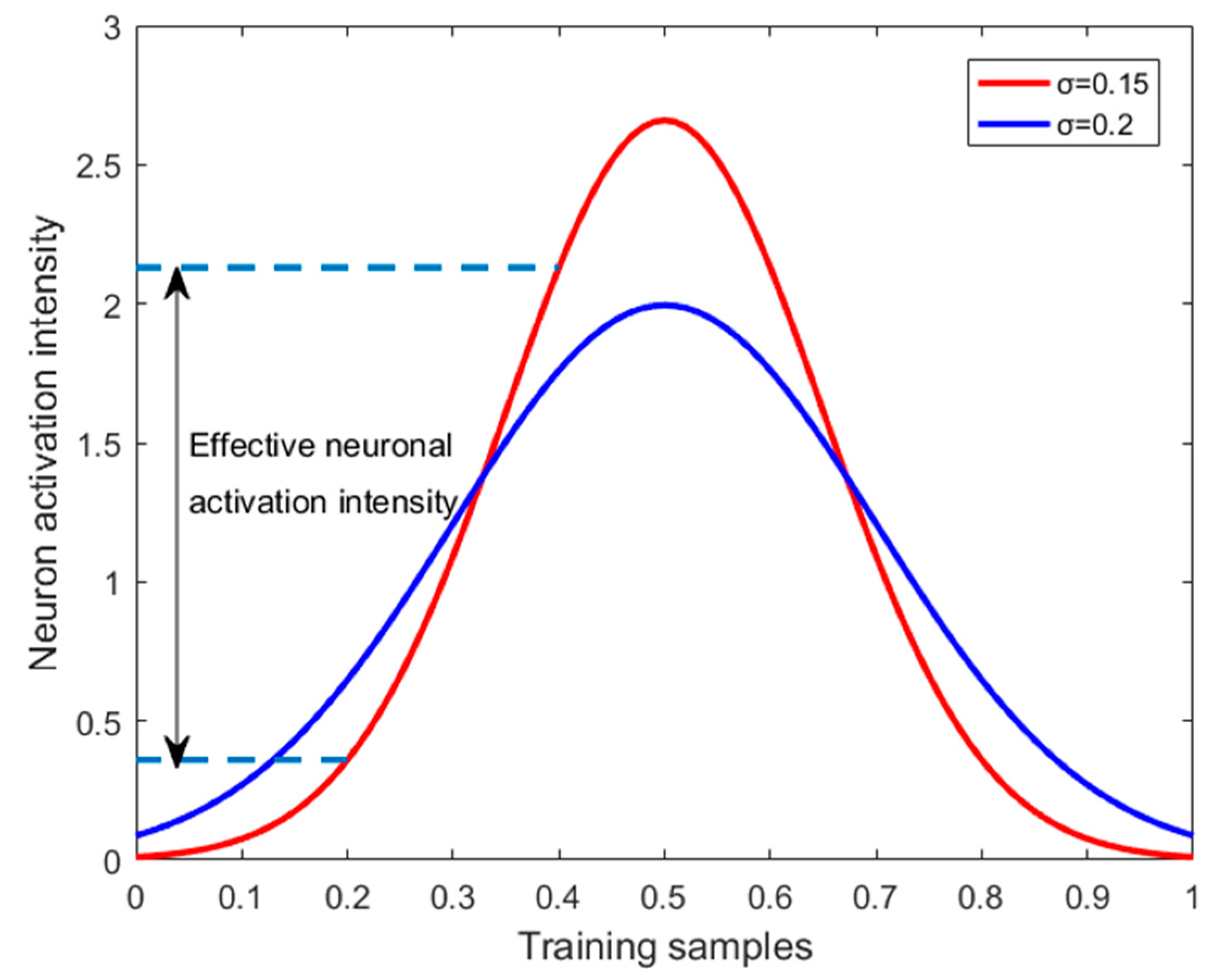
From Equation (17), it is known that when the sample is far from the neuron, the local field potential value of the sample is smaller, so the activation strength (AS) of the sample on the neuron is defined as
A S i = ( x i c i , J ) 2 σ i , J 2 , i = 1 , 2 , ,
where i is the dimension of the input sample, J is the number of center columns closest to the sample, and σ i , J is the width of the neuron.
According to Figure 2, the activation strength of neuron decays as the distance of the sample from the center increases. When the value of ASi as in Equation (19) is less than the minimum activation strength we set, and, here, the activation strength threshold is 0.2,
A S i < A S t h .
The center is not well-activated by the sample, and the ith dimensional generalization performance of the neuron is not good. Therefore, we expand the neuron width of the current center to improve its generalization, and the width growth parameter ε is set to 0.01
σ i , J = ( 1 + ε ) × σ i .
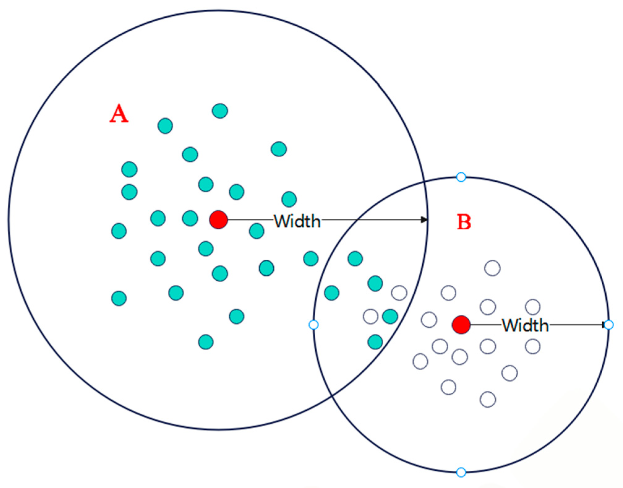
A large number of samples are gathered around an effective center. As the training samples enter, there is an overlap of samples [29], as shown in Figure 3. There is an overlap of samples attributed to centers A and B. Ref. [8] showed that the width of the MF neurons has a significant effect on the generalization performance of the system. If the width is too large, the MF neurons will have a large amount of overlap and will give a value close to 1 for the different input systems. Since the number of samples around neurons A and B differs, the activation strength of each sample for a neuron is also inversely proportional to the distance between the neurons. To evaluate the generalization properties of the MF neurons, the neuron density potential is defined as:
d e n s i t y _ p o t J = k = 1 p i = 1 , 2 , , m A S i m P ,
where the density potential energy increases or decreases with the number of neurons, and J denotes the nearest neuron marker to the sample.
If the density potential of a neuron is greater than the threshold we set, it means that the width of that central neuron can be appropriately converged in that neuron sample set to reduce redundancy. The density threshold is set according to the experiment, and the width convergence parameter δ is set to 0.01
d e n s i t y _ p o t J d e n _ t h ,
σ J = ( 1 δ ) × σ _ o r J ,
where σ _ o r J is the original width.

3.1.3. Neuron Deletion

According to the above analysis, the density potential energy can effectively reflect the activity of a neuron. If the density potential energy of a neuron is low, it proves that the center of the neuron is not a centroid with high density characteristics. Finding the neuron with the lowest density potential energy,
g = arg min 0 i m d e n s i t y _ p o t i ,
If the density potential does not satisfy the threshold, a pruning of the neuron is required, and the result is as follows:
d e n s i t y _ p o t g < I t h ,
d e l e t e   c g , σ g , w g , d e n s i t y _ p o t g .
The threshold value is mainly determined by experience, and, here, we set the threshold value to 1.

3.1.4. Merging of Network-Rule Neurons

After completing the adjustment of neuron width or updating the parameters, sometimes one or more pairs of neurons become highly similar. In order to obtain a highly compact model and avoid overfitting, a similarity calculation is required. Lughofer et al. [30] developed two methods of merging rules to eliminate local redundancy; the first is to merge the overcoincident clusters in the clustering space, and the other is to calculate the projection overlap of fuzzy sets in different dimensions, to merge any similar fuzzy sets. We belong to the second method, which calculates the similarity index of different input dimensions separately, so only the similarity index and the largest pair of neurons in all input dimensions will be merged. The similarity is calculated, mainly referring to the method in [31,32], where the ratio of the intersection and concatenation between a pair of neurons is defined as the similarity:
S ( A , B ) = i = 1 n M ( A i B i ) i = 1 n M ( A i B i ) ,
where S ( A , B ) represents the similarity between A and B fuzzy set, and Equation (27) indicates the intersection of A and B, rather than the concatenation of A and B.
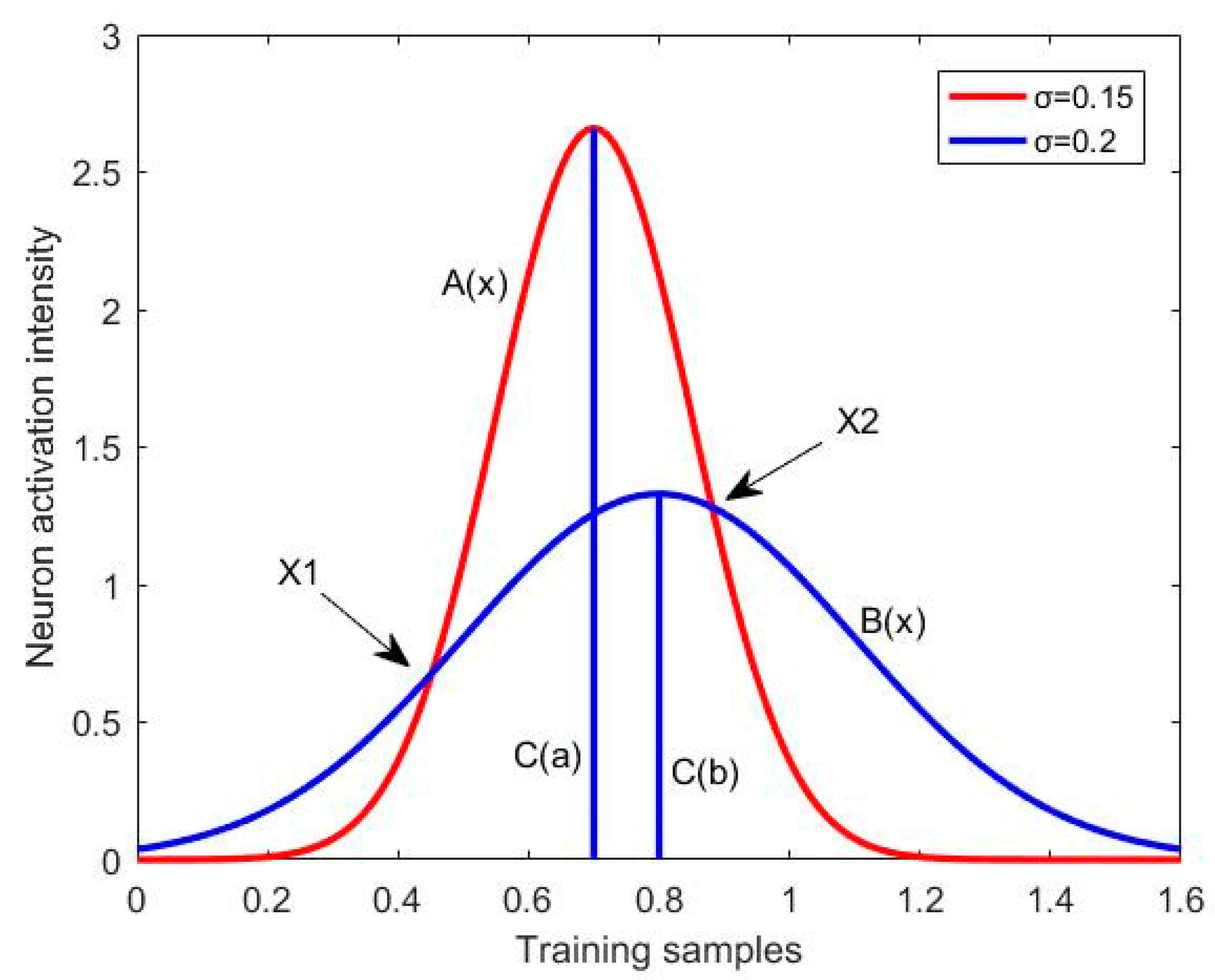
As shown in Figure 4, Gaussian function A(x) intersects with Gaussian function B(x) at points X1 and X2, and their centers are C(a) and C(b), respectively. The intersection of A and B is the area where the two Gaussian functions intersect:
M ( A i B i ) = a i b i μ A i B i ( x i ) d x i = a i X 1 μ A i ( x i ) d x i      + X 1 X 2 μ B i ( x i ) d x i X 2 b i μ A i ( x i ) d x i ,
M ( A i B i ) = a i b i μ A i B i ( x i ) d x i = a i X 1 μ B i ( x i ) d x i      + X 1 X 2 μ A i ( x i ) d x i X 2 b i μ B i ( x i ) d x i ,
According to [31], the integral item a b μ A ( x ) d x with Gaussian function μ a ( x ) can be calculated by the Gaussian error function, thus improving the computational efficiency:
a b μ A ( x ) d x = σ A π 2 [ e r f ( b c A σ A ) e r f ( a c A σ A ) ] ,
e r f ( x ) = 1 1 ( 1 + a 1 x + a 2 x 2 + a 3 x 3 + a 4 x 4 ) 4 , x 0 ,
where a1 = 0.278393, a2 = 0.278393, a3 = 0.278393, and a4 = 0.278393.
Calculate the similarity between each center and find the maximum value,
S q w = arg max 0 i , j m S i j ,
where q and w are the labels of similar neurons.
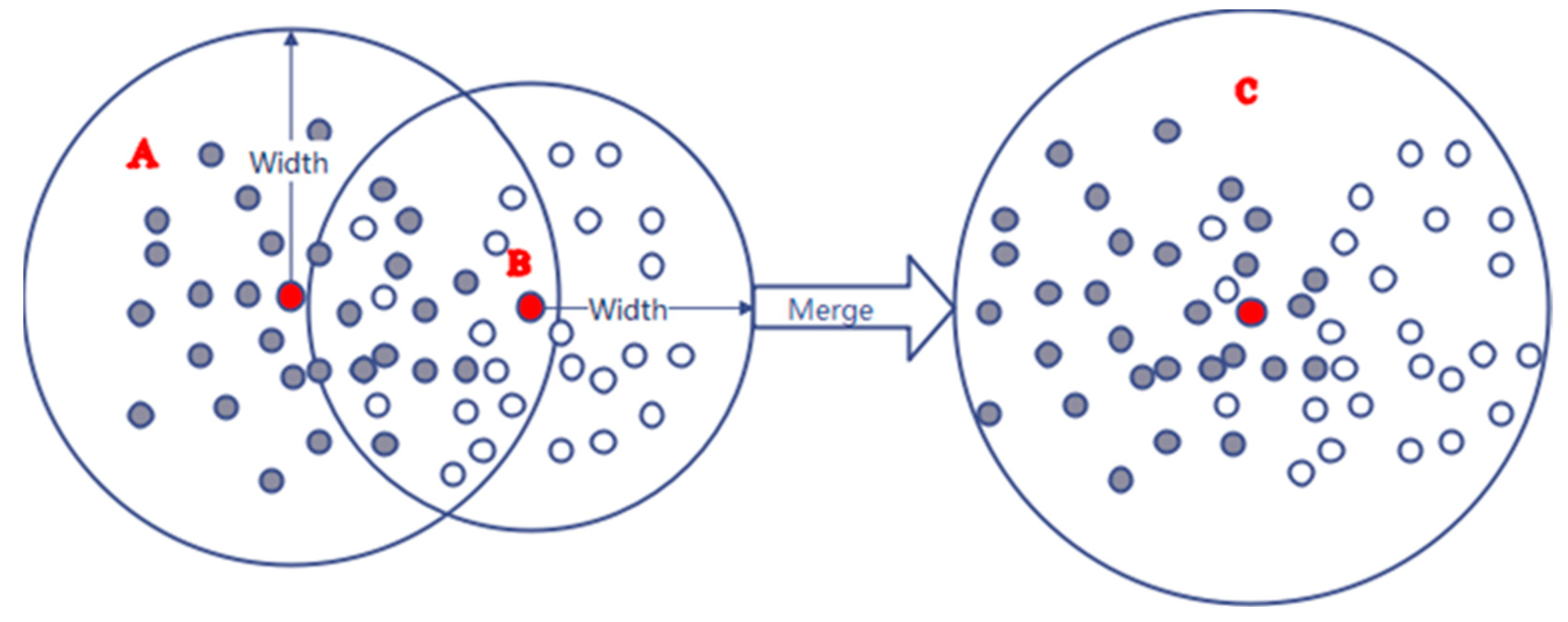
If the similarity of a pair of neurons is larger than the threshold, it means that there is a redundancy of centers, and we merge them into one with the number of neurons minus one, as shown in Figure 5, merging two neurons into one.
S q w > S t h .
The merged neuron is the mean value of the original neuron:
c n e w = ( c q + c W ) 2 ,
σ n e w = ( σ q + σ W ) 2 ,
w n e w = ( w q + w W ) 2 ,
d e n s i t y _ p o t n e w = ( d e n s i t y _ p o t q + d e n s i t y _ p o t W ) 2 .

3.2. Adaptive Second-Order Learning Algorithm

Currently, first-order optimization algorithms such as the error back-propagation (EBP) algorithm in [33] are widely used for parameter learning, but EBP tends to fall into the local minimum when dealing with large-scale computing problems. In order to improve the system performance, in this paper, we use the improved second-order LM algorithm proposed in [34] to implement parameter updates, combining it with the adaptive learning rate in [20], which can further speed up the convergence rate.
Each time a self-organizing operation is performed on a fuzzy neural network, the parameters need to be adjusted using a second-order algorithm,
ψ ( t + 1 ) = ψ ( t ) ( H ( t ) + λ ( t ) I ( t ) ) 1 Ω ( t ) .
where H is the quasi-Hessian matrix, λ ( t ) is the learning coefficient, I is an identity matrix, Ω denotes the gradient vector, and ψ denotes all parameters:
Ψ ( t ) = [ c 1 ( t ) , c 2 ( t ) , , c r ( t ) , σ 1 ( t ) , σ 2 ( t ) , , σ r ( t ) , ω 1 ( t ) , ω 2 ( t ) , , ω r ( t ) ] .
The adaptive learning coefficients are determined as,
λ ( t ) = ξ e p + ( 1 ξ ) Ω ( t ) ,
where is ξ a predefined constant, which can be set to 0.5 according to [17].
To reduce the computational complexity, the quasi-Hessian matrix and the gradient vector are computed as:
H ( t ) = p = 1 p h p ( t ) ,
Ω ( t ) = p = 1 P g p ( t ) ,
where the sub quasi-Hessian matrix and the sub gradient vector are calculated as:
h p ( t ) = j p T ( t ) j p ( t ) ,
g p ( t ) = j p T ( t ) e p ( t ) ,
where the error vector e p ( t ) can be obtained from Equation (13), and the Jacobi matrix j p ( t ) can be calculated as:
j p = [ e p c 11 , e p c 12 , , e p c 1 N , , e p c l N , e p σ 1 , , e p σ l , e p ω 1 , , e p ω l ] ,
where l is the number of rule layer, and N is the dimension of the input sample. Using the differential chain rule, the elements of the rows of the Jacobi matrix in Equation (45) can be rewritten as:
e p c l N = y p ^ c l N = 2 ω l θ l ( x p ) ( x p N c l N ) σ l
e p σ l = y p ^ σ l = 2 ω l θ l ( x p ) x p c l 2 σ 3 l
e p ω l = y p ^ ω l = θ l ( x p )
Algorithm 1 summarizes the specific implementation process of the network, including structural self-organization and parameter adjustment. Its flowchart is shown in Figure 6.
Algorithm 1: Pseudocodes for constructing SOFNN-CA network
Input: The input data in the training set are generally four inputs.
Output: Single output datum in training set.
  • Set a parameter for the number of clusters: ma_addth, e_min, den_th, and S_th
  • Using k-means clustering Formula (2) to initialize the network center
  • for p = 1 to n do
  • Calculate the error of the sample according to (13)
  • Update the parameters of the current network according to (38)
  • for k = 1 to n do
  • Calculate the error of the sample according to (13)
  • Calculate the RMSE according to (14)
  • end
  • if mod(p,5) = 0
  • if RMSE(k) > RMSE(k-1) and md_ind < md_addth
  • Add a new neuron according to (16)
  • end
  • Calculate neuron impact intensity and density potential energy according to (18), (21)
  • if AS < e_min
  • Updata width according to (20)
  • end
  • if den_pot > den_th
  • Updata width according to (23)
  • end
  • Calculate the Similarity index according to (27)–(31)
  • if S > S_th
  • Merge related neurons according to (34)–(37)
  • end
  • end
  • end

3.3. Convergence Analysis

In order to ensure proper operation in industrial applications, this section gives the convergence analysis of SOFNN-CA, which is mainly divided into a structure fixation phase and a structure dynamic-adjustment phase.
Assume that at moment t, the current error e(t) is:
e ( t ) = y ^ t y t .
Define the Lyapunov function as:
V ( Θ ( t ) ) = 1 2 e T ( t ) e ( t ) ,
Theorem 1.
There are fixed r neurons in the rule layer of SOFNN-CA. The parameters of SOFNN-CA are updated by (38), if
Δ Θ ( t ) min { Δ Θ ( t 1 ) , Ω ( Δ Θ ( t 1 ) ) Ψ ( Δ Θ ( t 1 ) ) } ,
then the convergence of SOFNN-CA can be maintained, and there is e(t)→0 as t→+∞.

3.3.1. Under a Fixed Structure

With Equation (38) updating the parameters, the deviation of the Lyapunov function at this point is
Δ V ( Θ ( t ) ) = V ( Θ ( t + 1 ) ) V ( Θ ( t ) ) = E T ( Θ ( t ) ) Δ Θ ( t ) + 1 2 Δ Θ T ( t ) 2 E ( Θ ( t ) ) Δ Θ ( t ) ,
where E T ( Θ ( t ) ) and 2 E T ( Θ ( t ) ) are the gradient vector and the second-order derivative matrix, respectively. According to Equation (52), the variation of the Lyapunov function can be rewritten as
Δ V ( Θ ( t ) ) = 1 2 Δ Θ T ( t ) 2 E ( Θ ( t ) ) Δ Θ ( t ) .
When Equation (51) is satisfied, since 2 E T ( Θ ( t ) ) is positive definite, we can obtain Δ V ( Θ ( t ) ) < 0 . Therefore,
lim t + e ( t ) = 0 .
So the SOFNN-CA is theoretically convergent.

3.3.2. Structural Dynamic Adjustment Phase

When the neuron increase mechanism is satisfied, a new neuron is added, at which point the new neuron is inserted into the regular layer. The MF layer neurons are increased from r to r+1, the approximation error of the neuron is e r + 1 ( t ) , and the width update formula in Equation (16) w j + 1 = e j ( t ) h j + 1 ( t ) is moved into Equation (55):
e r + 1 ( t ) = y p ( t ) j = 1 r + 1 w j ( t ) h j ( t ) = y p ( t ) ( j = 1 r w j ( t ) h j ( t ) + w r + 1 ( t ) h r + 1 ( t ) ) = e j ( t ) e j ( t ) h j + 1 ( t ) h j + 1 ( t ) = 0 .
Equation (55) shows that with the increase in time, when new neurons are inserted into the hidden layer, the setting of the weight parameter compensates for the output error of the network, and the adjusted error will not increase, which ensures the convergence of the system and can improve the training speed of the algorithm to a certain extent.
If the merging mechanism of neurons is satisfied, similar neurons will be merged. At this time, the number of MF layer neurons is r − 1, and the output error of the neural network is e r 1 ( t ) , using Equation (36) to obtain:
e ^ r 1 ( t ) = y p ( t ) j = 1 , j w r w j ( t ) h j ( t ) = y p ( t ) ( j = 1 , j q , w r w j ( t ) h j ( t ) + w q ( t ) h q ( t ) ) = y p ( t ) ( j = 1 , j q , w r w j ( t ) h j ( t ) + 1 2 w q ( t ) h q ( t ) + 1 2 w w ( t ) h q ( t ) ) = e r 1 ( t ) + ( 1 2 w q ( t ) h q ( t ) + w w ( t ) h w ( t ) 1 2 w w ( t ) h q ( t ) ) < 2 e r 1 ( t )
Since, after the merge operation, the error will not be greater than twice the original error, which varies within a reasonable range, and, as the iterative process progresses, the merged neuron no longer occurs, e(t)→0, the convergence of SOFNN-CA can be guaranteed.

4. Simulation Analysis

First, the proposed SOFNN-CA network is evaluated by chaotic system and dynamic nonlinear system identifications, and then the tested network is applied to two real prediction problems to provide an overall assessment of the network performance.
All simulations were written in MATLAB R2016b and run on a PC with a clock speed of 2.10 GHZ and 8 GB of memory in a Microsoft Windows 7 environment, and the root-mean-square error (RMSE) and average percentage error (APE) are introduced in this study [35],
A P E ( t ) = 1 P p = 1 P | y d p ( t ) y p ( t ) | | y d p ( t ) | × 100 % ,
where P is the number of test data.

4.1. Mackey–Glass Time-Series Forecasting

In the first benchmark test, we examine SOFNN-CA using chaotic Mackey–Glass time-series prediction [36]. This time series is generated by the differential delay equation:
x ( t + 1 ) = ( 1 a ) x ( t ) + b x ( t τ ) 1 + x 10 ( t τ )
where a = 0.1, b = 0.2, τ = 17, and x(0) = 1.2 in the initial condition, according to the description in the literature [25], and the prediction model can be described as follows:
x ( t + H ^ ) = f ¯ ( x ( t ) , x ( t 6 ) , x ( t 12 ) , x ( t 18 ) )
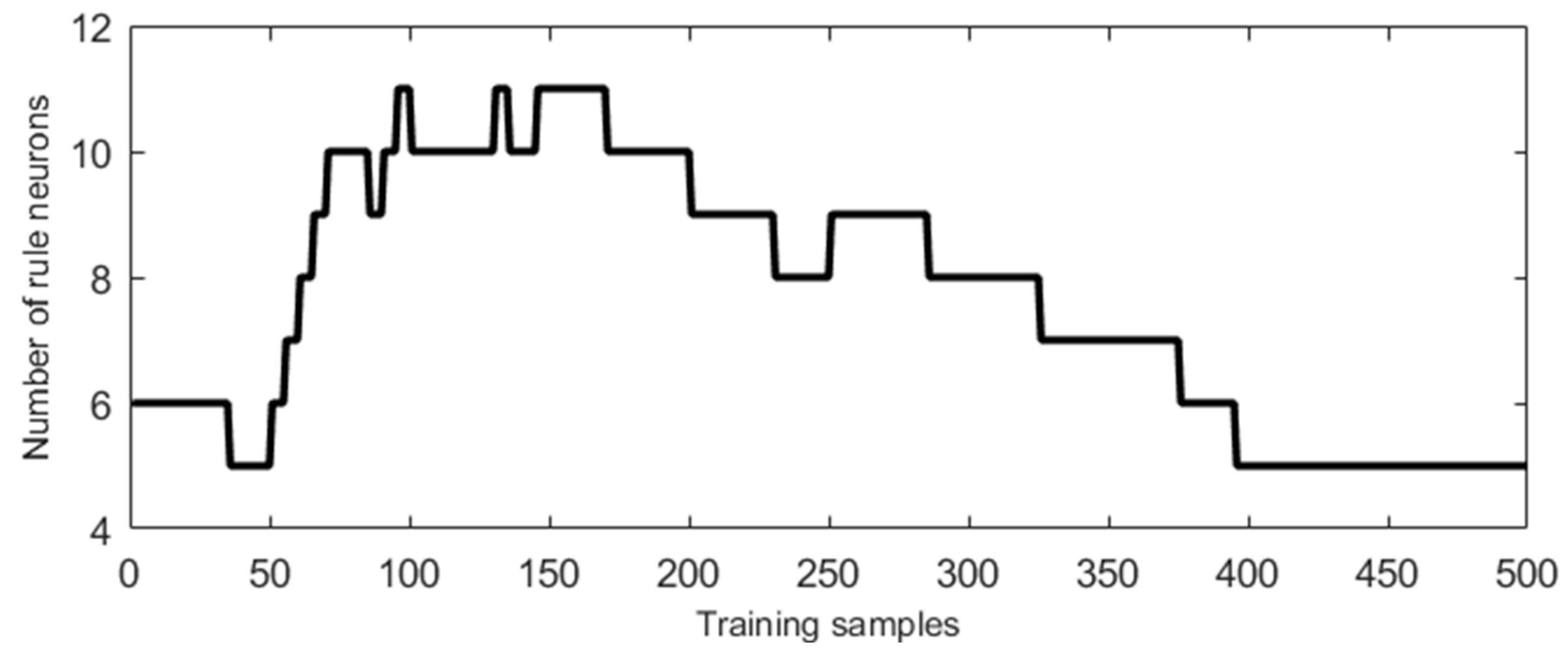
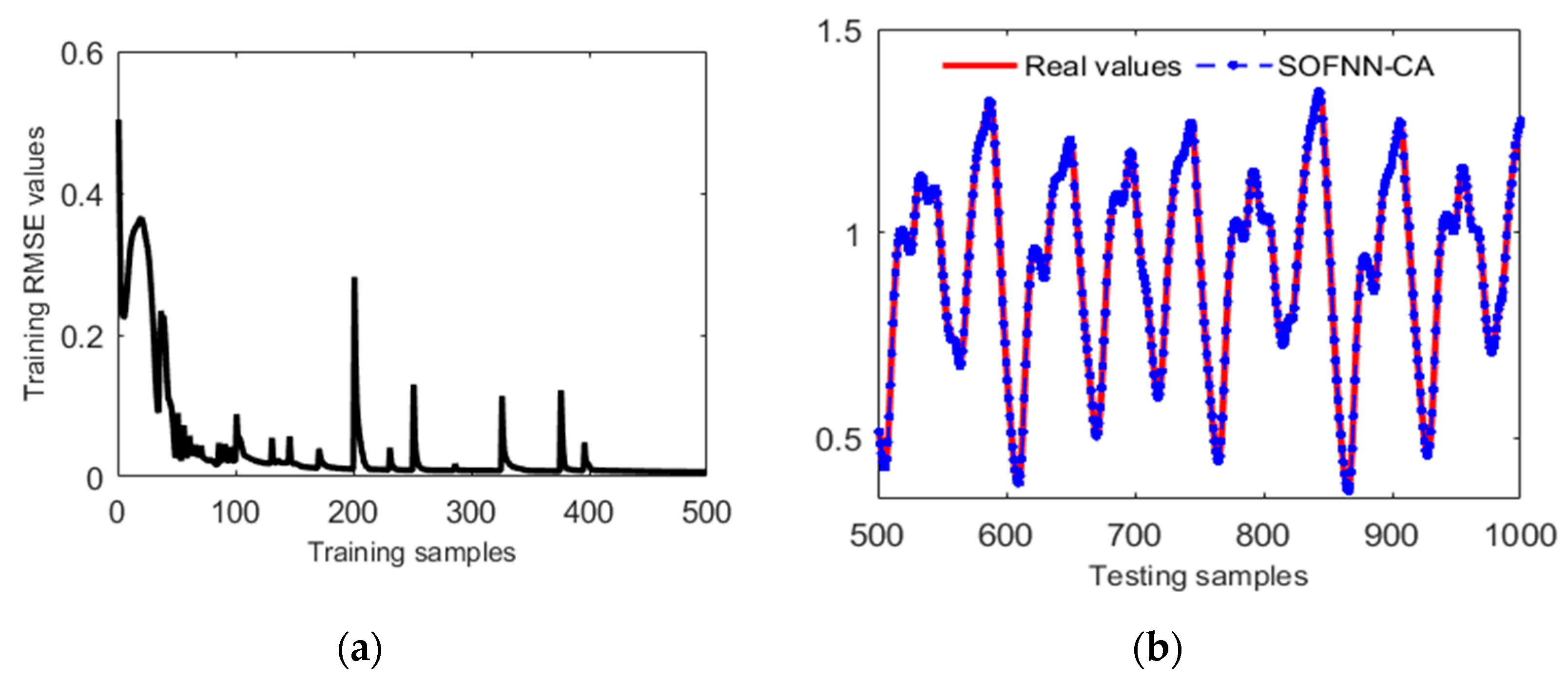
The 500 data pairs from t = 1 to 500 are selected as the training data set, and the remaining data pairs within the interval [501, 1000] are used as the test data set. In this experiment, we take k-means algorithm to generate six clusters, on which self-organized learning is performed. The parameters of the network are obtained by an empirical method, and the growth threshold ma_addth is set to 0.6, the width adjustment thresholds e_min and den_th are set to 0.2 and 10, respectively, and the merging threshold S_th is 7. The simulation results are shown in Figure 7 and Figure 8. The comparison algorithms use the same training and test samples listed in Table 1, and the results are the means of multiple tests.
Figure 7 shows the change of neurons as the number of iterations increases. The number of neurons first increases to 11 and then gradually decreases to 5, resulting from a self-organizing mechanism that learns the features of new samples and then merges similar neurons. From the curve of training the RMSE in Figure 8a, it can be seen that there are some peaks in the RMSE of SOFNN-CA, which are caused by merging neurons. Figure 8b shows that the method is effective. Furthermore, Table 1 lists the performance comparison details of SOFNN-CA and its competitors. It can be seen that the proposed SOFNN-CA obtained the best tested RMSE (0.0058) and the best tested APE (0.0055). Due to the neuronal merging mechanism, SOFNN-CA has the most compact network structure, and its performance is better than SOFNN-ALA, SOFNN-AGA, and SOFNN-ACA. Owing to the inherent drawbacks of the adopted EBP-based parameter optimization algorithm, although SOFNN-AGA, SOFNN-ACA, and FNN-EBP can achieve better test results, the training time is longer because more iterations are required to achieve the required accuracy. SOFNN-GA has the longest training time using the genetic algorithm. The results in Table 1 show that the SOFNN-CA proposed in this paper can obtain high prediction performance with a compact network structure.

4.2. Identification of Nonlinear Systems

In this example, the proposed SOFNN-CA is applied to identify dynamic systems with the following input delays [14]:
y ( t + 1 ) = 0.72 y ( t ) + 0.025 y ( t 1 ) u 1 ( t 1 ) + 0.01 u 1 2 ( t 2 ) + 0.2 u 1 ( t 3 ) .
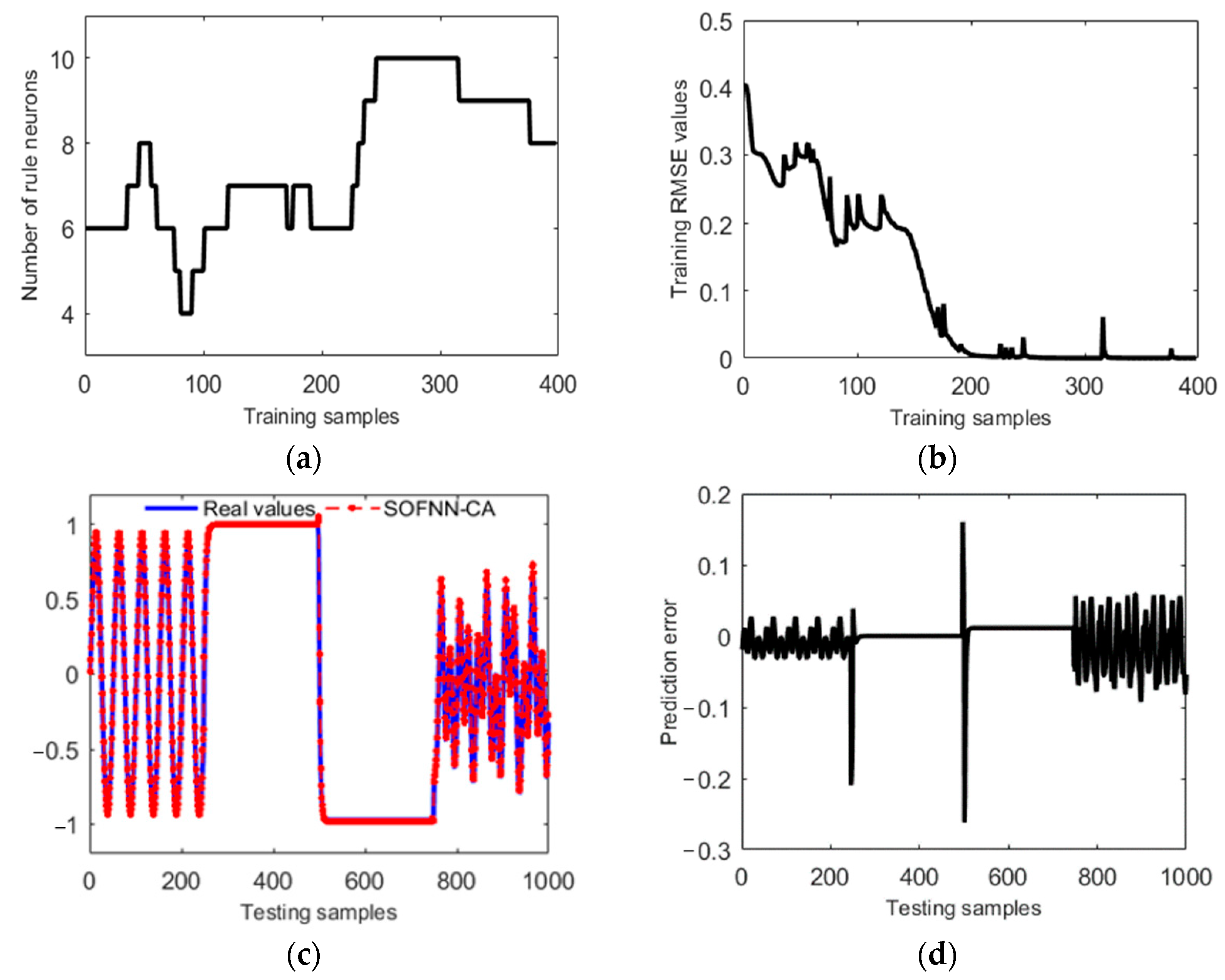
The initial state is y ( 1 ) = y ( 2 ) = y ( 3 ) = y ( 4 ) = 0 , and u ( t ) = 1.05 × sin ( t / 45 ) . Four variables y ( t ) , y ( t 1 ) , u 1 ( t 1 ) , and u 1 ( t 2 ) are selected as input samples, and e is the output samples, with a total of 1000 sets of data for training.The number of neurons after initialization using the k-means algorithm is six, and the thresholds are md-addth = 0.15, e-min = 0.2, den-th = 5, and S-th = 8, and the expected error e is 0.0001. After the training process, the following signal u(t) is used to test the performance of the proposed SOFNN-CA, in which there are 1000 sets of training samples. The comparison algorithms use the same training and test samples listed in Table 2, and the results are the means of multiple tests.
u ( t ) = { sin ( π t / 25 ) t < 250 1.0 250 t < 500 1.0 500 t < 750 0.3 sin ( π t / 25 ) + 0.1 sin ( π t / 32 ) + 0.6 sin ( π t / 10 )     750 y < 1000 .
The test results are shown in Figure 9.
Figure 9d shows the test error of the neural network, which varies slightly with different input functions. Since the input data is a dynamically changing function, the error is larger in the function segmentation region than in other regions.
It is shown in Table 2 that SOFNN-CA outperforms SOFNN-ALA in test accuracy, but increases in the number of neurons and training time. Due to the adaptive gradient descent algorithm, SOFNN-AGA requires more iterations under the same error standard as SOFNN-CA, and the training time is longer, while the training accuracy is almost the same.
Compared to RSEFNN-LF and FWNN algorithms, RSEFNN-LF uses an auto-evolutionary method to generate fuzzy rules online and uses the gradient descent algorithm to update the parameters, which builds a small number of neurons but is inferior to the SOFNN-CA algorithm in accuracy and training time. FWNN added a wavelet function to the subsequent part of the rule, which achieved better experimental results, but the performance was slightly worse than SOFNN-CA. Therefore, the present algorithm has good performance in the dynamic recognition of nonlinear systems compared with the other existing algorithms.

4.3. Combined Cycle Power-Plant Power-Output Forecast

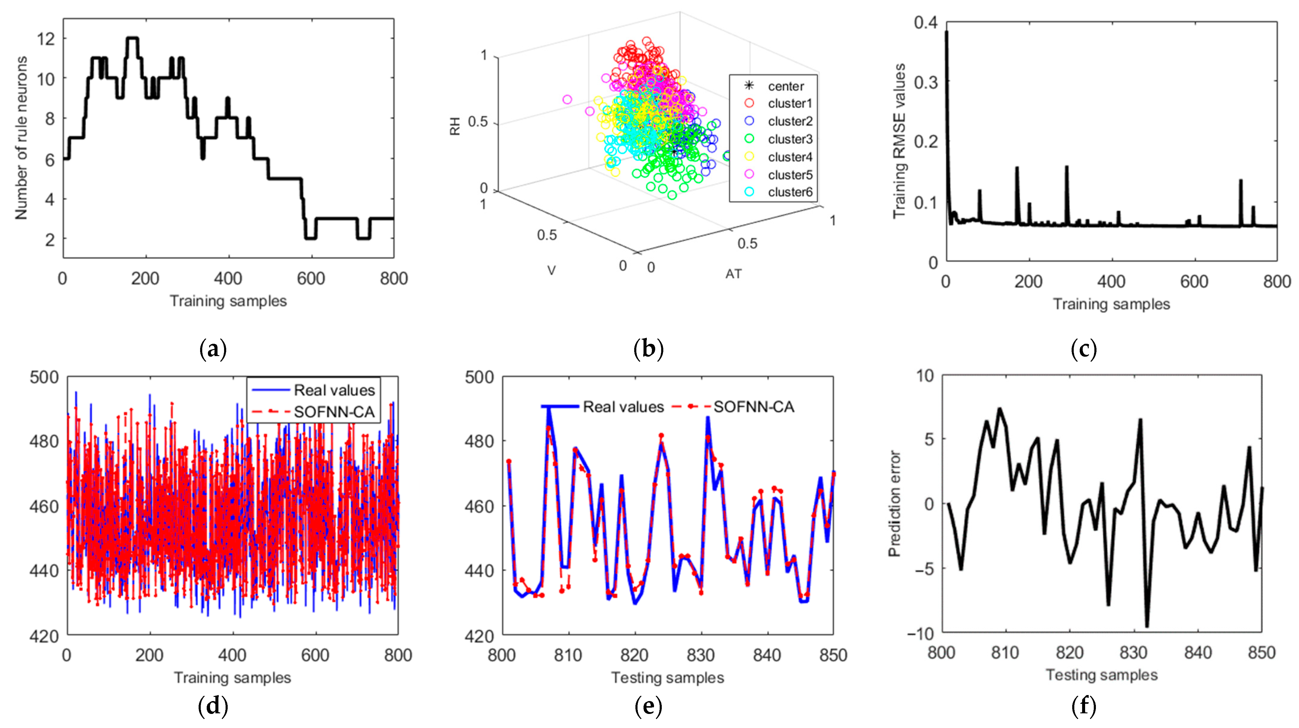
The above two tests are tested based on generic benchmark experiments, and in this experiment, we use data from a combined-cycle power plant [40] for testing. The data were obtained from the UCI machine learning dataset with temperature (T), ambient pressure (AP), relative humidity (RH), and exhaust vacuum (EV) as the input variables and electrical energy output (EEO) as the output variable. After removing the missing values, 850 samples are selected from the dataset, of which the first 800 samples are used for training, and the remaining 50 are used for testing. Since the input and output data have a wide range of values, they need to be normalized. The parameters of SOFNN-CA in this example are empirically set as follows: md-addth is 0.2, e-min is 0.2, den-th is 10, and S-th is 8. The training results are shown in Figure 10.
As shown in Figure 10a, the number of neurons is six in the initial condition, and SOFNN-CA increases and merges neurons under the action of a self-organization mechanism, to finally obtain a compact network structure of three neurons. The k-means initialization algorithm, as shown in Figure 10b, generated six clusters with different colors. The final test results are shown in Figure 10e, with errors in the [−10 10] interval.
The performance comparison between SOFNN-CA and the other algorithms is shown in Table 3. The proposed SOFNN-CA implements the simplest network structure (3 fuzzy rules) and the best test RMSE (3.6034). Among all the competitors, SOFNN-HPS adopts a hierarchical pruning self-organization method and has a good test RMSE (3.7469), but the number of neurons is twice that of SOFNN-CA due to the low efficiency of neuronal merging. DG-FNN and D-FNN have more fuzzy rules and a higher training accuracy, but the test accuracy becomes low, and the over-fitting phenomenon exists. Due to more parameters needing to be set, the test RMSE of GD-FNN is higher than that of D-FNN.
Compared with GEBF-OSFNN, the proposed SOFNN-CA can obtain better performance regarding the number of rules and test accuracy. This indicates that the proposed self-organization scheme can effectively merge similar fuzzy rules and achieve high generalization of neural networks.

4.4. Prediction of Benzene Levels in Air

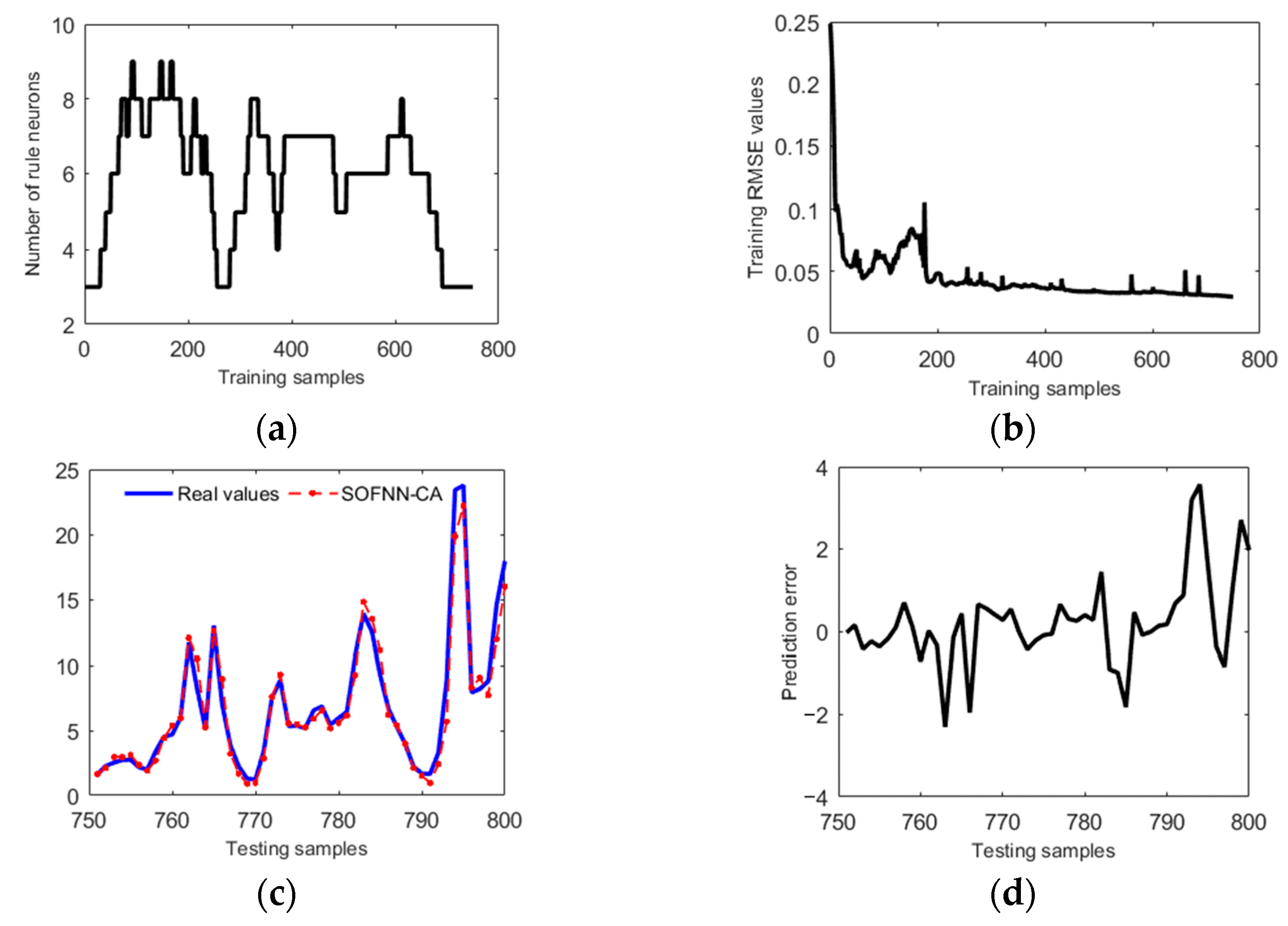
In this example, we use the air quality dataset from UCI [42,43]. This dataset contains responses from gas multisensor devices deployed at urban road sites in Italy with high levels of Class I pollutants and contains 1232 sets of hourly averaged response instances from five metal oxide chemical sensor arrays embedded in air quality chemical multisensor devices. After processing the missing values, we obtained 800 data, using 750 of them for training and 50 of them for testing. The input samples are carbon monoxide (CO), Non-Metanic Hydrocarbons (NMHC), Total Nitrogen Oxides (Nox) content, and air temperature (T) in the air, and the output is benzene (C6H6) content. The parameters of SOFNN-CA are set as follows: md-addth is 0.2, e-min is 0.2, den-th is 12, and S-th is 12. The experimental results are shown in Figure 11.
As can be seen from Figure 10a, the initial neurons generated by the clustering algorithm are set to three, and the number of neurons changes more obviously and stabilizes at the end. Figure 11b shows the RMSE of the training process, while Figure 11c shows the prediction results; it can be seen that the prediction accuracy is high, and the error is between [−3 3].
As shown in Table 4, with only three neurons, SOFNN-CA reaches the best test performance, and the RMSE is 1.0280. At the same time, the test error is smaller than the training error, indicating that the network has a strong generalization ability, and the neuron activation intensity index and density index helped to improve the generalization ability of the network. SOFNN-ALA has a smaller training error during training, but its generalization is weaker because the test error of the network is larger than the training error. ATO-RBF uses an error correction algorithm to increase the number of neurons, so more neurons must be added in order to reduce the error. Therefore, the network is larger, and its test error is 1.4900 higher than those of SOFNN-CA and SOFNN-ALA. It can be seen that the algorithm proposed in this paper has a better performance index. In the experiment of the prediction of benzene content in the air, the prediction can be achieved with high accuracy, and the practical problems can be solved effectively.

5. Conclusions

The object of this paper is to improve the real-time ability and generalization of nonlinear system modeling. SOFNN-CA is initialized by the k-means algorithm in the offline learning phase, which provides the training center parameters for the self-organization phase. In addition, we propose the MD index, neuron-based DPI, and AS index, which have low computational complexity and can achieve a fast and efficient self-organization mechanism. The parameter update adopts the improved adaptive LM algorithm, which has the advantages of fast convergence and a strong search capability, improving the learning speed. SOFNN-CA is tested by two benchmark problems and two real-world problems. The experimental results show that its prediction performance is greatly improved over the prediction performances of its competitors, where the network structure is more transparent, the training time is shorter, and the test performance is superior. SOFNN-CA can be applied to the online modeling of dataflow-based nonlinear systems, where the offline learning stage can be used to extract information from incomplete data.
The shortcoming of this study is that the adaptive setting of the parameter thresholds cannot be implemented, so the next steps of the study are to implement SOFNN-CA for the adaptive adjustment of thresholds, apply it to the prediction of ammonia nitrogen content in sewage treatment plants, and realize practical industrial tests.

Author Contributions

T.Z. suggested the idea of the work and designed the experimental method. Z.W. wrote the paper and performed the experiments. Both authors critically revised the paper. All authors have read and agreed to the published version of the manuscript.

Funding

This research is supported by the scientific research project of the Education Department of Liaoning Province, and the approval number is JDL2020013.

Data Availability Statement

Not applicable.

Conflicts of Interest

The authors declare no conflict of interest.

References

  1. Zeng, P.; Sun, F.; Liu, Y.; Wang, Y.; Li, G.; Che, Y. Mapping future droughts under global warming across China: A combined multi-timescale meteorological drought index and SOM-Kmeans approach. Weather. Clim. Extrem. 2021, 31, 100304. [Google Scholar] [CrossRef]
  2. Iyer, H. Model Discrimination for Nonlinear Regression Models. Technometrics 1990, 32, 448–450. [Google Scholar] [CrossRef]
  3. Aldeen, M.; Crusca, F. Modular Modelling of Nonlinear Complex Systems. In Proceedings of the 2003 4th International Conference on Control and Automation Proceedings, Montreal, QC, Canada, 12 June 2003; pp. 698–702. [Google Scholar]
  4. Sachtleben, R.; Peleska, J. Effective grey-box testing with partial FSM models. Softw. Test. Verif. Rel. 2022, 32, e1806. [Google Scholar] [CrossRef]
  5. Cecati, C.; Kolbusz, J.; Rozycki, P.; Siano, P.; Wilamowski, B.M. A Novel RBF Training Algorithm for Short-Term Electric Load Forecasting and Comparative Studies. IEEE Trans. Ind. Electron. 2015, 62, 6519–6529. [Google Scholar] [CrossRef]
  6. Akhtar, I.; Kirmani, S.; Ahmad, M.; Ahmad, S. Average Monthly Wind Power Forecasting Using Fuzzy Approach. IEEE Access 2021, 9, 30426–30440. [Google Scholar] [CrossRef]
  7. Czarnowski, I.; Jedrzejowicz, J.; Jedrzejowicz, P. Designing RBFNs Structure Using Similarity-Based and Kernel-Based Fuzzy C-Means Clustering Algorithms. IEEE Access 2020, 9, 4411–4422. [Google Scholar] [CrossRef]
  8. Zhou, H.; Zhang, Y.; Duan, W.; Zhao, H. Nonlinear systems modelling based on self-organizing fuzzy neural network with hierarchical pruning scheme. Appl. Soft Comput. 2020, 95, 106516. [Google Scholar] [CrossRef]
  9. Gholami, V.; Khaleghi, M.R.; Sahour, H.; Amri, M.A.H. Prediction of soil splash erosion using fuzzy network-CANFIS. Arab. J. Geosci. 2022, 15, 1604. [Google Scholar] [CrossRef]
  10. Han, H.-G.; Lin, Z.-L.; Qiao, J.-F. Modeling of nonlinear systems using the self-organizing fuzzy neural network with adaptive gradient algorithm. Neurocomputing 2017, 266, 566–578. [Google Scholar] [CrossRef]
  11. Wu, S.; Er, M.J.; Ni, M.; Leithead, W.E. A fast approach for automatic generation of fuzzy rules by generalized dynamic fuzzy neural networks. In Proceedings of the 2000 American Control Conference (ACC), Chicago, IL, USA, 28–30 June 2000; Volume 4, pp. 2453–2457. [Google Scholar]
  12. Wu, S.; Er, M.J. Dynamic fuzzy neural networks-a novel approach to function approximation. IEEE Trans. Syst. Man Cybern. Part B Cybern. 2000, 30, 358–364. [Google Scholar] [CrossRef]
  13. Han, H.; Zhang, L.; Wu, X.; Qiao, J. An Efficient Second-Order Algorithm for Self-Organizing Fuzzy Neural Networks. IEEE Trans. Cybern. 2017, 49, 14–26. [Google Scholar] [CrossRef]
  14. Han, H.; Wu, X.-L.; Qiao, J.-F. Nonlinear Systems Modeling Based on Self-Organizing Fuzzy-Neural-Network With Adaptive Computation Algorithm. IEEE Trans. Cybern. 2013, 44, 554–564. [Google Scholar] [CrossRef]
  15. Wang, G.; Qiao, J. An Efficient Self-Organizing Deep Fuzzy Neural Network for Nonlinear System Modeling. IEEE Trans. Fuzzy Syst. 2021, 30, 1. [Google Scholar] [CrossRef]
  16. Lughofer, E. Evolving fuzzy systems: Fundamentals, reliability, interpretability, useability and applications. In Proceedings of the 2015 7th International Joint Conference on Computational Intelligence (IJCCI), Lisbon, Portugal, 12–14 November 2015; p. 11. [Google Scholar]
  17. Škrjanc, I.; Iglesias, J.A.; Sanchis, A.; Leite, D.F.; Lughofer, E.D.; Gomide, F. Evolving fuzzy and neuro-fuzzy approaches in clustering, regression, identification, and classification: A Survey. Inf. Sci. 2019, 490, 344–368. [Google Scholar] [CrossRef]
  18. Lin, Y.-C.; Lee, S.-J.; Ouyang, C.-S.; Wu, C.-H. Air quality prediction by neuro-fuzzy modeling approach. Appl. Soft Comput. 2019, 86, 105898. [Google Scholar] [CrossRef]
  19. Leng, G.; McGinnity, T.M.; Prasad, G. Design for Self-Organizing Fuzzy Neural Networks Based on Genetic Algorithms. IEEE Trans. Fuzzy Syst. 2006, 14, 755–766. [Google Scholar] [CrossRef]
  20. Zhou, H.; Zhao, H.; Zhang, Y. Nonlinear system modeling using self-organizing fuzzy neural networks for industrial applications. Appl. Intell. 2020, 50, 1657–1672. [Google Scholar] [CrossRef]
  21. Lughofer, E. Improving the robustness of recursive consequent parameters learning in evolving neuro-fuzzy systems. Inf. Sci. 2020, 545, 555–574. [Google Scholar] [CrossRef]
  22. Yu, H.; Wilamowski, B.M. Neural Network Training with Second Order Algorithms. In Human—Computer Systems Interaction: Backgrounds and Applications 2; Hippe, Z.S., Kulikowski, J.L., Mroczek, T., Eds.; Springer: Berlin, Heidelberg, 2012; Volume 99, pp. 463–476. [Google Scholar]
  23. Qiao, J.; Meng, X.; Li, W. An incremental neuronal-activity-based RBF neural network for nonlinear system modeling. Neurocomputing 2018, 302, 1–11. [Google Scholar] [CrossRef]
  24. Caron, M.; Misra, I.; Mairal, J.; Goyal, P.; Bojanowski, P.; Joulin, A. Unsupervised Learning of Visual Features by Contrasting Cluster Assignments. arXiv 2021, arXiv:2006.09882. [Google Scholar]
  25. Fei, J.; Wang, T. Adaptive fuzzy-neural-network based on RBFNN control for active power filter. Int. J. Mach. Learn. Cybern. 2018, 10, 1139–1150. [Google Scholar] [CrossRef]
  26. Milstein, J.N.; Koch, C. Dynamic Moment Analysis of the Extracellular Electric Field of a Biologically Realistic Spiking Neuron. Neural Comput. 2008, 20, 2070–2084. [Google Scholar] [CrossRef] [PubMed] [Green Version]
  27. Lughofer, E.; Cernuda, C.; Kindermann, S.; Pratama, M. Generalized smart evolving fuzzy systems. Evol. Syst. 2015, 6, 269–292. [Google Scholar] [CrossRef]
  28. Ghorbani, H. Mahalanobis distance and its application for detecting multivariate outliers. Facta Univ. Ser. Math. Inform. 2019, 34, 583–595. [Google Scholar] [CrossRef]
  29. Xie, S.; Xie, Y.; Huang, T.; Gui, W.; Yang, C. Generalized Predictive Control for Industrial Processes Based on Neuron Adaptive Splitting and Merging RBF Neural Network. IEEE Trans. Ind. Electron. 2018, 66, 1192–1202. [Google Scholar] [CrossRef]
  30. Lughofer, E.; Bouchot, J.-L.; Shaker, A. On-line elimination of local redundancies in evolving fuzzy systems. Evol. Syst. 2011, 2, 165–187. [Google Scholar] [CrossRef]
  31. Li, W.; Qiao, J.; Zeng, X.-J. Online and Self-Learning Approach to the Identification of Fuzzy Neural Networks. IEEE Trans. Fuzzy Syst. 2020, 30, 649–662. [Google Scholar] [CrossRef]
  32. Li, W.; Qiao, J.; Zeng, X.-J. Accurate similarity analysis and computing of Gaussian membership functions for FNN simplification. In Proceedings of the 2015 12th International Conference on Fuzzy Systems and Knowledge Discovery (FSKD), Zhangjiajie, China, 15–17August 2015; pp. 402–409. [Google Scholar]
  33. Wilamowski, B.M. Modified EBP algorithm with instant training of the hidden layer. In Proceedings of the IECON’97 23rd International Conference on Industrial Electronics, Control, and Instrumentation (Cat. No.97CH36066), New Orleans, LA, USA, 14 November 1997; Volume 3, pp. 1097–1101. [Google Scholar]
  34. Yu, H.; Wilamowski, B.M. Levenberg–Marquardt Training. In Intelligent Systems; Wilamowski, B.M., Irwin, J.D., Eds.; CRC Press: Boca Raton, FL, USA, 2018; pp. 12–16. [Google Scholar]
  35. Kreinovich, V.; Nguyen, H.T.; Ouncharoen, R. How to Estimate Forecasting Quality: A System-Motivated Derivation of Symmetric Mean Absolute Percentage Error (SMAPE) and Other Similar Characteristics. 2014. Available online: https://scholarworks.utep.edu/cs_techrep/865/ (accessed on 6 August 2022).
  36. Glass, L.; Mackey, M. Mackey-Glass equation. Scholarpedia 2010, 5, 6908. [Google Scholar] [CrossRef]
  37. Malek, H.; Ebadzadeh, M.M.; Rahmati, M. Three new fuzzy neural networks learning algorithms based on clustering, training error and genetic algorithm. Appl. Intell. 2012, 37, 280–289. [Google Scholar] [CrossRef]
  38. Juang, C.-F.; Lin, Y.-Y.; Tu, C.-C. A recurrent self-evolving fuzzy neural network with local feedbacks and its application to dynamic system processing. Fuzzy Sets Syst. 2010, 161, 2552–2568. [Google Scholar] [CrossRef]
  39. Abiyev, R.H.; Kaynak, O. Fuzzy Wavelet Neural Networks for Identification and Control of Dynamic Plants—A Novel Structure and a Comparative Study. IEEE Trans. Ind. Electron. 2008, 55, 3133–3140. [Google Scholar] [CrossRef]
  40. Tüfekci, P. Prediction of full load electrical power output of a base load operated combined cycle power plant using machine learning methods. Int. J. Electr. Power Energy Syst. 2014, 60, 126–140. [Google Scholar] [CrossRef]
  41. Wang, N. A Generalized Ellipsoidal Basis Function Based Online Self-constructing Fuzzy Neural Network. Neural Process. Lett. 2011, 34, 13–37. [Google Scholar] [CrossRef]
  42. De Vito, S.; Massera, E.; Piga, M.; Martinotto, L.; Di Francia, G. On field calibration of an electronic nose for benzene estimation in an urban pollution monitoring scenario. Sens. Actuators B 2008, 129, 750–757. [Google Scholar] [CrossRef]
  43. De Vito, S.; Piga, M.; Martinotto, L.; Di Francia, G. CO, NO2 and NOx urban pollution monitoring with on-field calibrated electronic nose by automatic bayesian regularization. Sens. Actuators B 2009, 143, 182–191. [Google Scholar] [CrossRef]
  44. Meng, X.; Zhang, Y.; Qiao, J. An adaptive task-oriented RBF network for key water quality parameters prediction in wastewater treatment process. Neural Comput. Appl. 2021, 33, 11401–11414. [Google Scholar] [CrossRef]
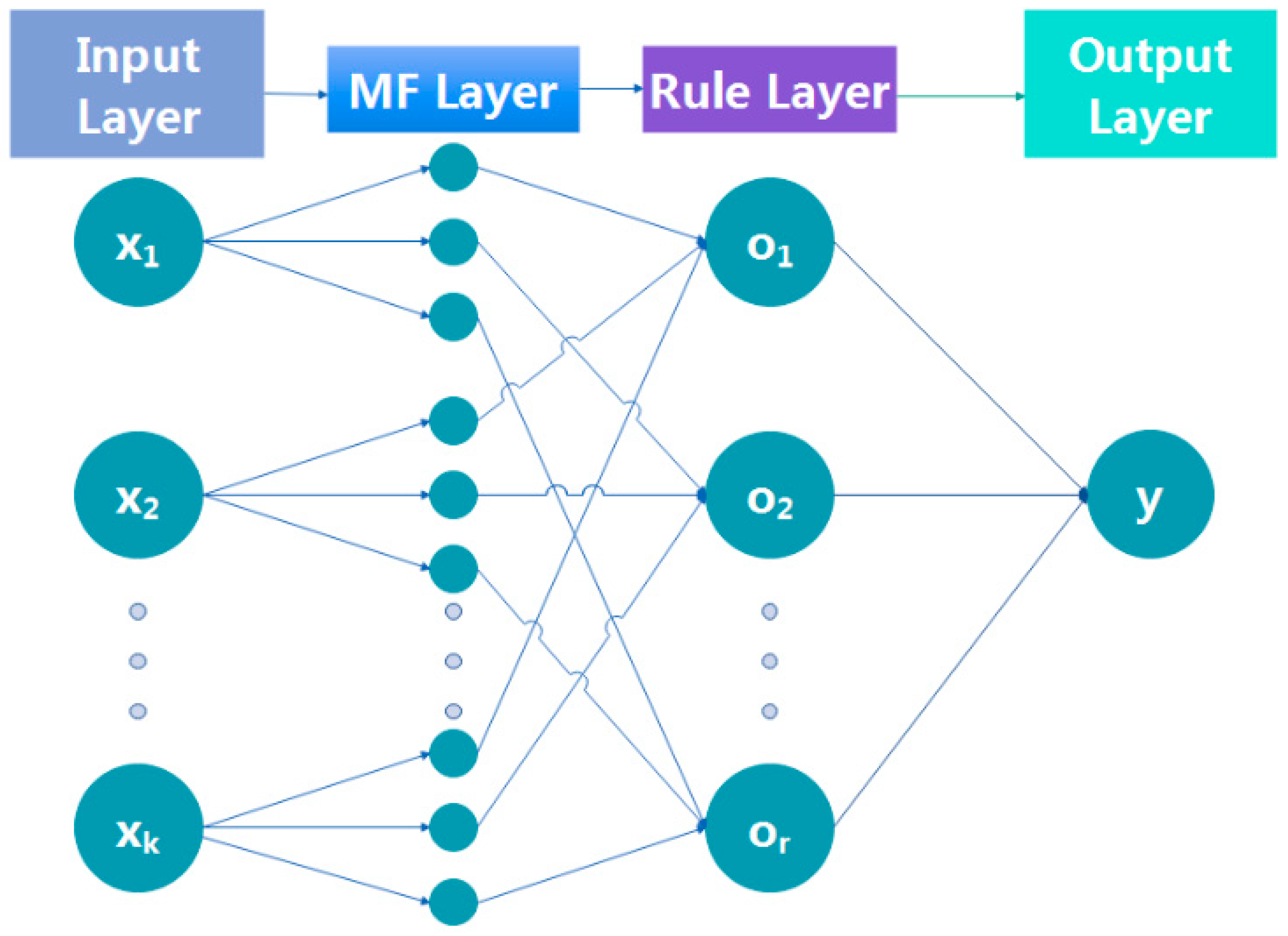
Figure 1. Fuzzy neural network structure diagram.
Applsci 12 11435 g001
Figure 2. Neuron activation strength.
Applsci 12 11435 g002
Figure 3. Diagram of the neural network center(bullets represent samples around neurons, and A and B represent two adjacent neurons).
Applsci 12 11435 g003
Figure 4. Relative position diagram of neurons A and B.
Applsci 12 11435 g004
Figure 5. Schematic diagram of neuronal merger(A and B are overlapping neurons, and C is the merged neuron).
Applsci 12 11435 g005
Figure 6. The flowchart of SOFNN-CA.
Applsci 12 11435 g006
Figure 7. Neuron number change graph.
Applsci 12 11435 g007
Figure 8. (a) Training RMSE chart; (b) test results chart.
Applsci 12 11435 g008
Figure 9. (a) Training neuron change plot; (b) training RMSE plot; (c) test result plot; (d) test error plot.
Applsci 12 11435 g009
Figure 10. (a) Neuron change plot; (b) k-means clustering plot; (c) training RMSE plot; (d) training result plot; (e) test result plot; (f) test error plot.
Applsci 12 11435 g010
Figure 11. (a) Training neuron change plot; (b) training RMSE plot; (c) test result plot; (d) test error plot.
Applsci 12 11435 g011
Table 1. Comparison results of different methods for predicting Mackey–Glass Time-Series.
MethodRule NeuronsTesting RMSETesting APECPU Times (s)
SOFNN-CA50.00580.00556.62
SOFNN-ALA [20]60.00660.00587.24
SOFNN-AGA [10]60.01190.007621.20
SOFNN-ACA [14]70.02010.007627.33
SOFNN-GA [19]70.01320.0094168.35
FNN-EBP [37]80.01420.013137.05
Table 2. Comparison results of different methods for identifying nonlinear system.
MethodRule NeuronsTesting RMSETesting APECPU Times (s)
SOFNN-CA80.01710.04905.11
SOFNN-ALA [20]60.02970.09543.73
SOFNN-AGA [10]60.00900.046413.10
RSEFNN-LF [38]4 10.0280 10.0652 135.31 1
FWNN [39]5 10.0201 10.0904 137.72 1
1 The results are listed in the original papers.
Table 3. Comparison of different methods under M-G experiment.
MethodRule NeuronsTraining RMSETesting RMSECPU Times (s)
SOFNN-CA34.16163.603411.26
SOFNN-HPS [8]74.07183.7469-
GEBF-OSFNN [41]9 14.2483 13.8327 1-
GD-FNN [11]15 13.8945 14.8510 1-
D-FNN [12]19 13.7485 14.2545 1-
1 The results are listed in the original papers.
Table 4. Comparison of different methods in benzene-content prediction.
MethodRule NeuronsTraining RMSETesting RMSECPU Times (s)
SOFNN-CA31.27091.028016.8202
SOFNN-ALA [20]51.18221.248115.7461
ATO-RBF [44]181.76431.4900-
Publisher’s Note: MDPI stays neutral with regard to jurisdictional claims in published maps and institutional affiliations.