Predicting the Wafer Material Removal Rate for Semiconductor Chemical Mechanical Polishing Using a Fusion Network

Abstract

Predicting the wafer material removal rate (MRR) is an important step in semiconductor manufacturing for total quality control. This work proposes a deep learning model called a fusion network to predict the MRR, in which we consider separating features into shallow and deep features and use the characteristics of deep learning to perform a fusion of these two kinds of features. In the proposed model, the deep features go through a sequence of nonlinear transformations and the goal is to learn the complex interactions among the features to obtain the deep feature embeddings. Additionally, the proposed method is flexible and can incorporate domain knowledge into the model by encoding the knowledge as shallow features. Once the learning of deep features is completed, the proposed model uses the shallow features and the learned deep feature embeddings to obtain new features for the subsequent layers. This work performs experiments on a dataset from the 2016 Prognostics and Health Management Data Challenge. The experimental results show that the proposed model outperforms the competition winner and three ensemble learning methods. The proposed method is a single model, whereas the comparison methods are ensemble models. Besides the experimental results, we conduct extensive experiments to analyze the proposed method.

1. Introduction

As with the popularity of electronic equipment, semiconductor manufacturing is becoming increasingly important these days. Many complex and sophisticated processes are involved in semiconductor manufacturing, among which chemical mechanical polishing (CMP) is the foundation of wafer fabrication [1,2]. It is worth mentioning that CMP has been recognized as a critical process for improving the production efficiency of semiconductor manufacturing processes [3]. Unlike pure mechanical and pure chemical polishing, CMP combines mechanical and chemical functions to avoid the surface damage and lengthy polishing process of pure mechanical polishing [4]. In the presence of pressure and a polishing slurry, the wafer and polishing pad rotate in opposite directions to synergistically combine the abrasive action of the particles in the slurry and the corrosive action of the oxidant to form a smooth surface on the wafer [5]. With a smooth surface, the wafers will be allowed to set up additional circuit elements on their flat surfaces in subsequent semiconductor manufacturing processes. Note that the output of the CMP process is the material removal rate (MRR), which refers to the surface quality of the polished wafers and the quality of the CMP process [6]. The unit of the MRR is usually expressed in nm/min to represent the thickness (nanometer) of the film removed per minute.

Taking into account the complicated interactions of the chemical and mechanical processes, many relevant parameters are related to the MRR including the slurry (e.g., flow rate and cohesion), operating environment (e.g., humidity and temperature), mechanism (e.g., rotational speed and pressure), polishing pad (e.g., thickness and heat resistance level), and membrane (e.g., hardness) [7,8,9]. Therefore, developing a predictive model with enormous process parameters is a valuable and challenging task.

The last decade has witnessed the outstanding progress of deep learning, which enables models to learn feature representations and perform classifications simultaneously [10]. This can reduce the overhead caused by manual feature extraction, which is used by traditional machine learning methods. Thus, this work proposes a deep learning model called the fusion network to predict the MRR in which data science approaches are used to analyze the data. We consider separating the features into shallow and deep features instead of using the samples with all the features as inputs. Our developed model aims to use the characteristics of deep learning to merge these two types of features. In the developed model, the deep features go through a sequence of nonlinear transformations and the goal is to learn the complex interactions among the features to obtain the deep feature embeddings. Additionally, the proposed method incorporates domain knowledge into the model by encoding the knowledge as shallow features. Once the learning of deep features is completed, the proposed model combines the shallow features and the deep feature embeddings learned to obtain new features for the subsequent layers.

We conduct experiments on the dataset obtained from the 2016 Prognostic and Health Management (PHM) Data Challenge, collected by virtual metrology (VM) technology to evaluate the proposed method. In the experiments, we compare our proposed method with the winner of the competition and with three ensemble learning methods. Compared to the comparison methods that use ensemble learning to combine several base models to boost model performance, our proposed fusion network comprises only a single model. However, the proposed model can still outperform the alternatives.

The contributions of this work are as follows:

• The proposed method is a deep learning model that can incorporate domain knowledge into the model by encoding the knowledge as shallow features. Additionally, the remaining features can go through a deep neural network to learn discriminative feature embeddings.
• The experiments are performed on the dataset from the 2016 PHM Data Challenge. To the best of our knowledge, the performance based on the proposed model outperforms all other methods in the existing literature.
• Finally, the prediction accuracy of the proposed method is demonstrated through extensive experiments.

The rest of this paper is organized as follows. Section 2 presents related surveys and techniques. Section 3 introduces the proposed method. Section 4 shows the experimental results and detailed discussions. Finally, the conclusions and future work are summarized in Section 5.

2. Related Work

Over the past decade, many studies have been proposed that consider the parameters and circumstances involved in the polishing process from the perspectives of the physical and chemical processes. Wang et al. [11] investigated the effects of the pH, oxidizer concentration, and slurry flow rate on the MRR. They showed that a higher oxidizer concentration or a higher slurry flow rate resulted in a higher MRR when the CMP was completed. This can be explained by an adhesive removal mechanism on the molecular scale. Jeng and Huang [12] discovered the cross-effect between the abrasion, wafer, particle size, and pad in the microcontact view, in which the sources of pressure are the pad deformation and number of abrasive particles. They also considered the relationship between the wafer surface hardness, slurry concentration, and slurry particle size. Oliver et al. [13] and Park et al. [14] investigated how the roughness of the pad surface affected the material removal process in CMP and discovered and explained the relationship between the MRR and the level of surface roughness of the pad. Ng et al. [15] developed an analytical MRR model to scale key process variables and replicated the surface finishing task performed by the manual operator. Dambon et al. [16] investigated how the wafer material affects the MRR by conducting mechanistic experiments and showed that the removal level is determined by the wafer deformation capability rather than the material hardness of the wafer. Thus, if the wafer material has a higher deformation ability, a higher MRR is obtained. Oh and Seok [17] presented an integrated MRR model of the MRR for silicon dioxide in CMP with the slurry chemical diffusion model. By comparing the results with the experimental dataset in the literature, the validity of the proposed model was supported.

The last decade has witnessed great progress in machine learning because of the advances in machine learning and the presence of big data [18,19,20]. The key idea behind machine learning is to learn predictive models from the data [21]. Once the learning process has been completed, the learned models make predictions on unseen data. Due to the growing demand for the accuracy, stability, and reliability of VM, many machine learning models, such as linear regression (LR), multivariate linear regression (MLR), multitask learning, and artificial neural networks, are commonly used in VM [22,23,24,25].

To cope with the problem that a model involves enormous features, feature selection is a commonly used technique. The goal is to select a subset of features from the original feature set. For example, to avoid the negative effects of many features, Hirai and Kano [26] used partial least squares (PLS) and variable importance in the projection to process 57,600 features, in which PLS was applied to find the fundamental relationship between features and output. Their proposed model tried to find the multidimensional direction in the feature space that explained the maximum multidimensional variance direction in the output space by removing the redundant features until the remaining number of features reached the target number. Tsai et al. [27] focused on the chemical–mechanical process for polishing a color filter (CMP-CF). They proposed an adaptive network-based fuzzy inference system with sliding-level particle swarm optimization (SL-PSO) to optimize the CMP-CF parameters.

In the 2016 PHM Data Challenge, Di et al. [28] discovered two new types of features that can improve prediction accuracy. The first feature was the “Time Neighbor Features” since they found out that there exists a strong correlation between the MRR at time t, that is, MRR(t), and MRR at $t-1$, that is, MRR($t-1$). The relationship can be extended to the previous time steps. The second feature was the “Usage Neighbor Features”, which is based on the usage of wafers. To obtain the usage neighbors, one has to calculate the mean values for the usage variables of each wafer; then, the K-nearest neighbors can be obtained based on the mean values.

Using the statistical features and the two types of features mentioned above, the authors significantly improved the prediction of the MRR. Their proposed method was an ensemble of multiple machine learning algorithms and won the first prize in the competition. In addition, another data-driven technique in the competition was proposed by Wang et al. [29], in which they used a deep belief network (DBN) to develop the model. The developed model was a stack of restricted Boltzmann machines (RBMs) with two layers, including visible and hidden layers, to extract the features, followed by a predictive model with a feed-forward three-layer neural network to make the predictions. Yu et al. [30] employed a physics-informed machine learning approach to forecasting the MRR more precisely. The proposed model determined the two attributes, the contact between the polishing pad and the abrasive, as well as the contact between abrasives and wafers, by combining a physics-based model and a data-driven model.

3. Proposed Method

We followed the flow of data science to design the predictive model, as shown in Figure 1. First, we removed outliers to avoid model bias toward those data samples with extreme values. The next step was to use the feature engineering technique to extract more meaningful features from the data. Once the feature engineering process was completed, the final step was to train the proposed fusion network using the available data samples with new features.

3.1. Dataset

The dataset used in the experiments was from the 2016 PHM Data Challenge, which was held by the PHM Society. Over the last few decades, the PHM has attracted much attention as an effective method of avoiding unnecessary maintenance operations and advancing safety reliability and availability [31]. The dataset comprises data collected during the various runs of the CMP tool for specific wafers over time. The 2016 PHM Data Challenge focused on tracking the health status of components within a wafer chemical mechanical polishing (CMP) system, which plays a critical role in improving the production efficiency of semiconductor manufacturing processes. Detailed information on the available process features is available on the PHM Data Challenge website (2016 PHM Data Challenge: https://www.phmsociety.org/events/conference/phm/16/data-challenge (accessed on 29 April 2021)). Data are presented in the form of comma-separated values (CSV) in which each row of data represents an instance of all measurement variables at any given time. In addition to the data, the competition separately provided an average rate of material removal from a wafer, which was measured in terms of the thickness of the material before and after CMP polishing.

In the dataset, the wafers are separated into two groups according to the MRR range: low-speed mode and high-speed mode. The MRR range for low-speed mode is about 50–110 (nm/min) and about 140–170 (nm/min) for high-speed mode. Moreover, the group of low-speed mode data can be further segmented into two different groups based on stage ID: Stages A and B. Figure 2 shows the MRR distribution of the dataset. The segmentation information and sample size for each group are listed in

Table 1. Segmentation information and sample size for each group in which the unit for the MRR range is nm/min.

Group	Chamber ID	Stage ID	MRR Range	Sample Size
				Training	Testing
High-speed	1, 2, 3	A	138–163	431	73
Low-speed (A)	4, 5, 6	A	53–89	983	165
Low-speed (B)	4, 5, 6	B	53–102	987	186

.

3.2. Outlier Detection

Data pre-processing is essential in data science since data samples may comprise outliers or noise. Data cleaning can remove these data samples to help the subsequent data analysis. Besides data cleaning, data transformation and integration are also essential to data pre-processing, and the goal is to obtain a dataset that is ready for model training.

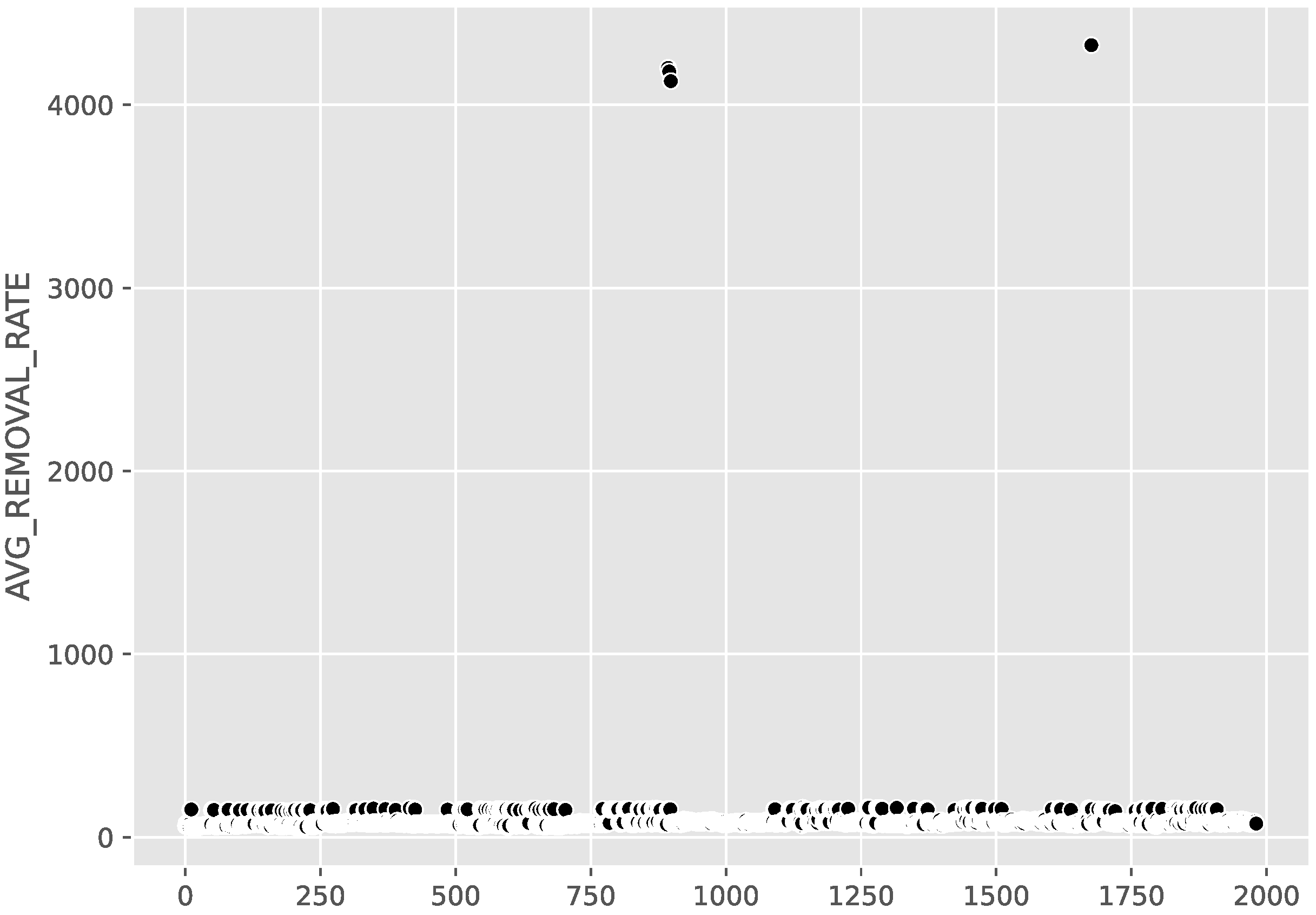
Outlier detection is an essential process in data analysis and this work used data visualization techniques to observe the data, as the information can be clearly and effectively analyzed through graphical means. Figure 3 shows the visualization results of the data samples in the 2016 PHM Data Challenge dataset. It is apparent that several data points are far from the rest of the data points so they are the outliers of the data samples. This work simply removed these outliers from the data samples since the MRRs of most wafers were below 170, whereas the MRRs for these outliers were more than 4000.

3.3. Feature Engineering

Once the data pre-processing was completed, we applied the feature engineering technique to extract the statistical measures from the pre-processed features, and the goal was to create more valuable features. In particular, feature engineering was crucial to the performance of the subsequent machine learning algorithms.

In addition to the original features, we included the descriptive statistics of the features in the feature set, including the maximum, minimum, mean, median, and standard deviation of the feature values. In addition, this work also included the aforementioned features, “Time Neighbor Features” and “Usage Neighbor Features”, in the feature set. The number of neighbor features was 20.

As seen in Table 1, it is apparent that the stage feature helped the model to make predictions since when the stage was B, the MRR was in low-speed mode. In contrast, the MRR could be in high- or low-speed modes when the stage was A. The stage is a discrete variable so we applied the one-hot-encoding technique to transform the stage feature into two features, “STAGE_A” and “STAGE_B”, and their values could be 1 or 0. Next, we removed the stage feature from the original features.

3.4. Fusion Network

In the previous section, we used the feature engineering technique to create more features. A practitioner can typically understand which features are essential for model training using visualization techniques or statistical analysis. For those identified as essential features, the model should use them directly during model training. In contrast, the model can use a deep neural network to extract essential features from the remaining features that do not have explicit information.

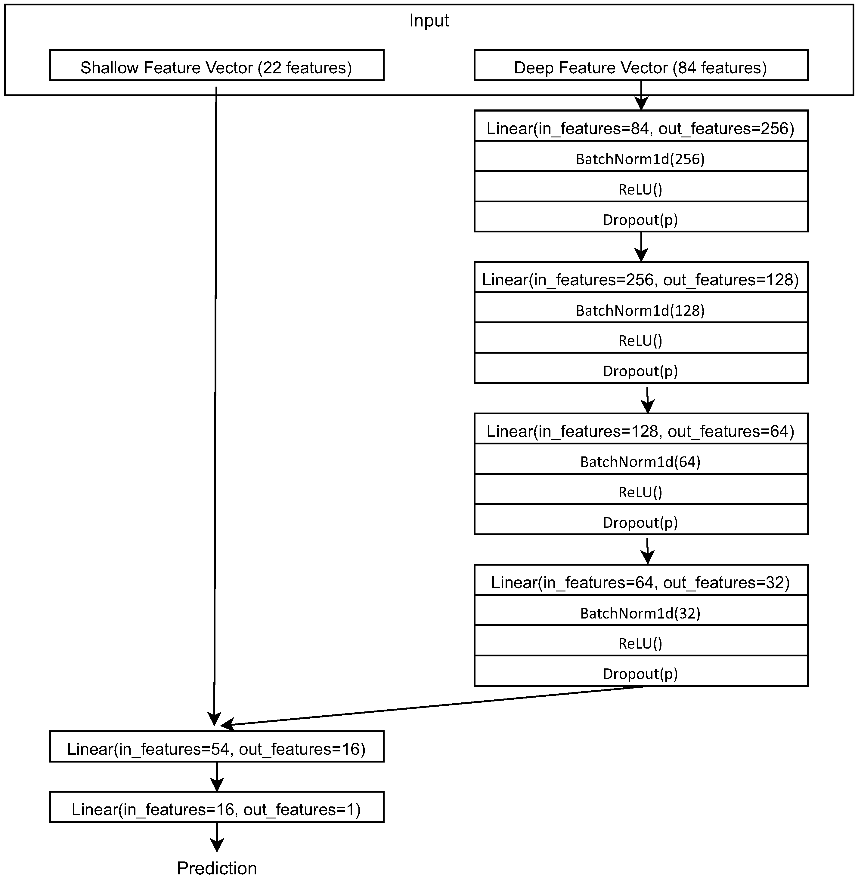
Thus, this work proposes a deep learning model called a fusion network to realize the idea. We separated the features into shallow and deep features, where the shallow features were those considered important, whereas the deep features required further nonlinear transformation. Figure 4 shows the architecture of the fusion network. This work used the neighbor features and one-hot-encoding of the stage feature as the shallow features, whereas the remaining features were considered deep features. All data samples comprised 22 shallow features and 84 deep features.

In our developed model, we used a series of fully connected layers, namely the linear layer shown in Figure 4, to perform the nonlinear transformation. It can be seen in Figure 4 that the deep features had to go through four layers so this work used several approaches to prevent the model from overfitting.

First, we applied the min-max normalization technique to transform the features by scaling each feature to the range of −1 and 1 so that features with large values did not dominate the model training. Second, each linear layer was followed by a batch normalization layer. Training a deep neural network tends to use a batch size of data samples as input and this can inject noise into each gradient update while achieving relatively fast convergence [32,33] from GPU parallelism. However, when the weights are updated, the distribution of the inputs to the deep layers of the network may change. This phenomenon is called the internal covariate shift, which leads to a decrease in actual learning efficiency. Ioffe et al. [34] presented batch normalization to mitigate the effect of unstable gradients within deep neural networks. Given the batch input x, the formula is shown below in Equation (1):

$$x^{*}=\frac{x-E\left[x\right]}{\sqrt{Var\left[x\right]+ϵ}}\times \gamma +\beta ,$$

(1)

where $x^{*}$ is the new value after normalization, $E\left[x\right]$ is the mean within a batch, $Var\left[x\right]$ is the variance within a batch, $ϵ$ is an arbitrarily small constant for numerical stability, and $\gamma$ and $\beta$ are learnable parameters.

Third, we used the rectified linear unit (ReLU) [35] activation function to perform the nonlinear transformation. ReLU is probably one of the most commonly used activation functions, as it can significantly accelerate model convergence [36] and alleviate the problem of the vanishing gradient. The formula of the ReLU function is shown below in Equation (2):

$$\mathrm{ReLU}\left(x\right)=max(0,x)$$

(2)

Finally, we applied the dropout [37] technique to the layers to randomly drop out neurons during the model training phase. At each training epoch, neurons were ignored with a probability p, forcing the neural network to learn more robust features. In particular, we applied batch normalization, the ReLU activation function, and dropout with a probability of $0.1$ to all the layers of the deep neural network, as shown in Figure 4, in which $p=0.1$ was obtained from cross-validation. The experiments further analyzed the influence of the dropout probability and batch normalization on model performance.

Once the learning of deep features was completed, we concatenated the shallow features and deep feature embeddings that passed through the deep neural network. Subsequently, we used two simple linear layers to fuse these two kinds of features. The final output was a scale value, as the prediction of the MRR is a regression problem. The loss function $\mathcal{L}$ used in the proposed model was the mean square loss, as shown in Equation (3):

$$\begin{array}{c}\hfill \mathcal{L}=\frac{1}{B}\sum _{i=1}^B{(y_i-{\widehat{y}}_i)}^2,\end{array}$$

(3)

where B is the batch size, $y_i$ is the label, and ${\widehat{y}}_i$ is the prediction result.

4. Results and Discussions

This work performed several experiments to evaluate and analyze the proposed method. First, we compared the proposed method with the winner of the 2016 PHM Data Challenge. Additionally, we compared our proposed method with several previous works on this dataset, including the methods proposed by Di et al. [28], Jia et al. [38], and Zhang et al. [39], respectively. Besides these methods, we used three state-of-the-art ensemble methods as the comparison methods. It is worth mentioning that the work conducted by Di et al. was also an ensemble method that comprised several base methods. In addition, we conducted extensive experiments to analyze our proposed method, which are discussed in this section.

4.1. Comparison Methods

Di et al. [28] combined the persistent model, K-nearest neighbor (kNN), linear regression, tree bagging, and support vector regression (SVR) models to develop an integrated model. The weight for each base model was defined by the prediction error obtained from the cross-validation, and the model that yielded better performance in the cross-validation was given a higher weight.

Jia et al. [38] employed a group method of data handling (GMDH)-type polynomial neural network for MRR prediction. The GMDH-type polynomial neural network was designed to effectively capture manufacturing information and address the problem of the high data dimensionality of the VM data. The final results indicated that their proposed method could further improve the prediction accuracy and outperform the random forest (RF), SVR, kNN, and logistic regression models.

Zhang et al. [39] constructed the convolutional neural network (CNN) and the residual convolutional neural network (ResCNN) to implement automatic feature extraction and weight sharing through the convolution and pooling layers from which superior prediction performance was obtained. ResCNN achieved the best performance in their experiments.

In addition, we further used three state-of-the-art ensemble methods as comparison methods. The first was RF, an ensemble method for classification, regression, and other tasks, which combines numerous decision trees. The key idea behind RF is to use a bootstrap sampling technique to generate enormous training sets, each of which is used to train a decision tree. To increase the diversity of the decision trees, the features of each decision tree are also obtained from a feature sampling set.

The second one was the gradient-boosting regressor, based on the gradient-boosted decision tree (GBDT). It combines many weak learners to form a strong learner iteratively. At each iteration, a regression tree is fitted to the negative gradient of the loss function. The final one was extreme gradient boosting (XGBoost) [40], which is an extension of the GBDT. It has become one of the most popular algorithms in data science competitions. The objective function of XGBoost comprises training loss and regularization, in which regularization can help the model avoid overfitting. On the other hand, XGBoost has improved this problem by using the second-order Taylor expansion of the loss function, making the tree more complex and powerful in learning. Moreover, XGBoost uses ${\ell }_1$ and ${\ell }_2$ as the regularization terms to help prevent the model from overfitting.

4.2. Evaluation Metric

This work used the mean squared error (MSE) shown in Equation (4) to evaluate the performance of the model, as the prediction of the MRR is a regression problem. Notably, the MSE was also the metric used in the competition. A smaller MSE means that an estimate is more accurate.

$$\begin{array}{c}\hfill MSE=\frac{1}{n}\sum _{i=1}^n{(y_i-\widehat{y_i})}^2,\end{array}$$

(4)

where n is the size of the estimates, $y_i$ is the ground truth, and $\widehat{y_i}$ is the predicted result.

Besides the MSE, the mean absolute error (MAE) that measures the difference between $y_i$ and $\widehat{y_i}$ is another metric for the evaluation of our proposed method. Equation (5) shows the definition of the MAE. Like the MSE, a smaller MAE means that an estimate is more accurate.

$$\begin{array}{c}\hfill MAE=\frac{1}{n}\sum _{i=1}^n|y_i-\widehat{y_i}|.\end{array}$$

(5)

4.3. Experimental Results

This section compares our proposed model with several state-of-the-art methods and the 2016 PHM Data Challenge winner. In the experiments, we used the training data provided by the competition and further split them into a training set and a validation set. The splitting ratio for the two sets was 9:1. Then, we used the training set to train the model and the validation set to tune the model parameters.

In our proposed model, the dropout probability p was 0.1 during the training phase. In addition, we used the Adam optimizer with an initial learning rate of 0.01 and a weight decay of 0.01. Setting the learning rate is a key step in deep learning and this work used a learning rate scheduler to control the learning rate, where the learning rate decreased by a factor of 10 when there was no improvement for five epochs. The batch size was 16 and the number of epochs was 100 for the fusion network in all experiments. The hyperparameters used by our proposed model are listed in

Table 2. Hyperparameters of the Proposed Model.

Parameter	Description
Dropout probability	0.1
Optimizer	Adam
Initial learning rate	0.01
Batch size	16
Number of epochs	100
Activation function	ReLU
Loss function	${\ell }_1$ Loss

. As for the other comparison methods, the best combination of hyperparameters was obtained using the grid search technique.

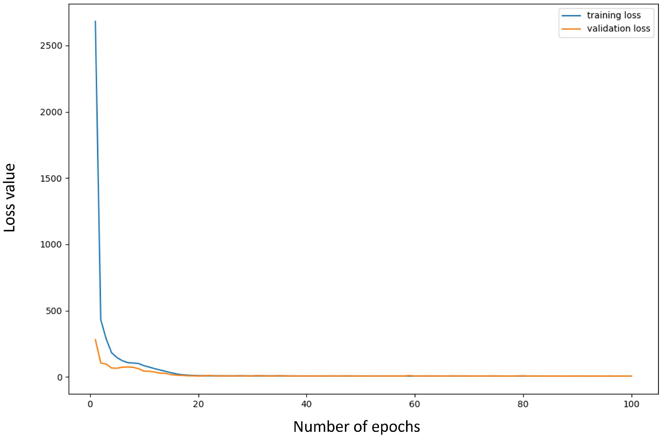
Additionally, Figure 5 shows the loss curves of our proposed model in which the y-axis is the loss value, whereas the x-axis denotes the number of epochs. It can be seen that both the training loss and the validation loss decreased as the number of epochs increased.

The experimental results are listed in

Table 3. Experimental results on the 2016 PHM dataset.

Methods	MSE	MAE
Di et al. [28]	7.07	N/A
Jia et al. [38]	6.62	N/A
Zhang et al. [39]	6.72	N/A
Random Forest	6.69	1.96
Gradient Boosting Regressor	6.78	1.96
XGBoost	6.66	1.94
Our proposed method	6.36	1.87

, indicating that our proposed method outperformed the alternatives. We conclude that the reasons why our proposed model outperformed that of Di et al. [28] are twofold. First, we used the data science approach to identify outliers and generate more discriminative features using the feature engineering technique. Second, the proposed model allowed practitioners to incorporate the findings from the data exploration step or knowledge into the network. Subsequently, the proposed fusion network used different routes to deal with shallow and deep features. Combining these two features enabled the model to benefit from the characteristics of deep neural networks to learn discriminative features. It is worth mentioning that the work of Di et al. [28] and the other three ensemble methods are based on ensemble learning, whereas the proposed method is a single model.

4.4. Fusion Network vs. Shallow Network vs. Deep Network

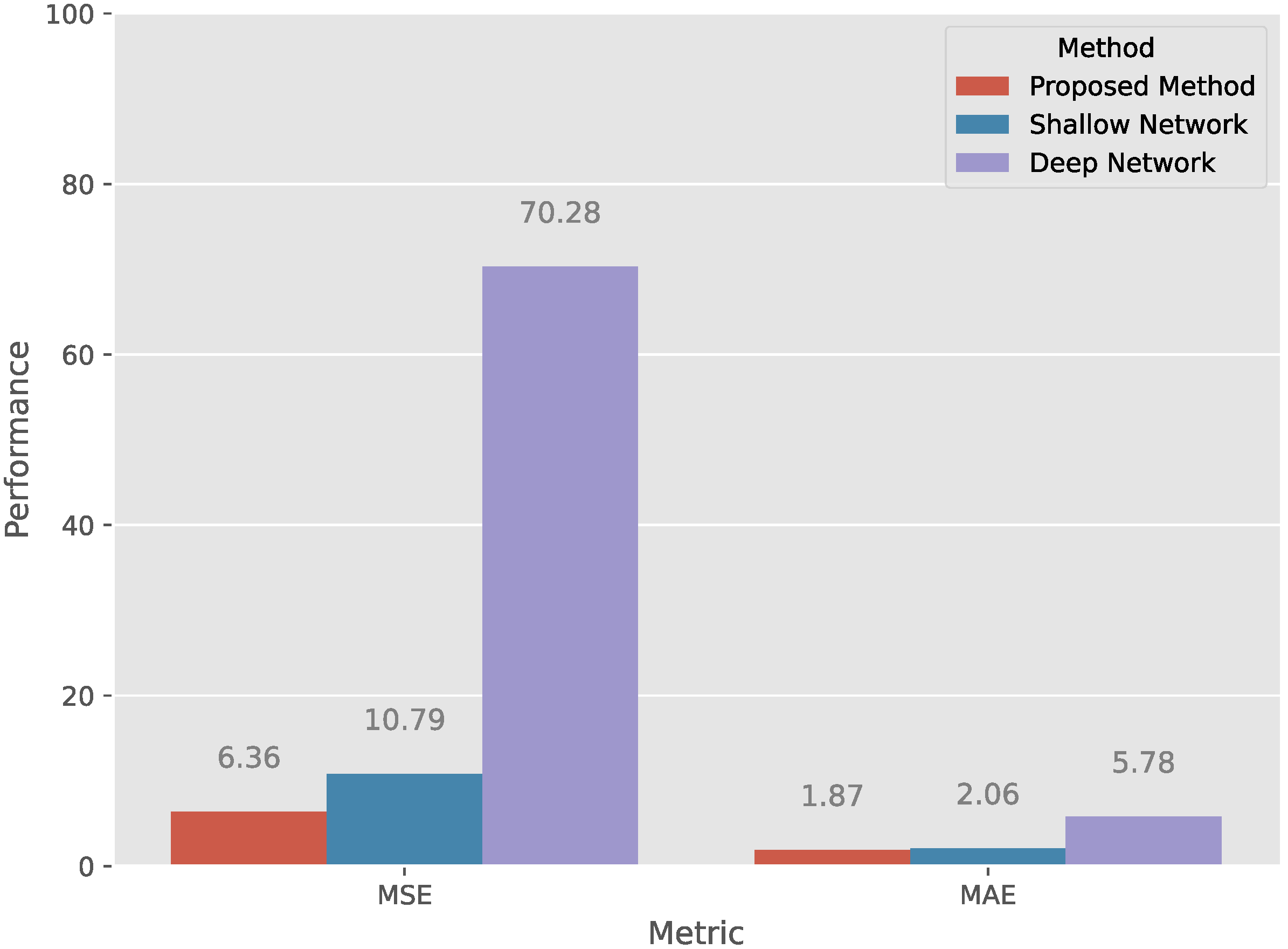
The proposed fusion network comprises two networks: a shallow network and a deep network. We conducted experiments to investigate the performance improvement caused by these two networks. In the design of the deep network, all features go through the deep network, namely the right network of the fusion network, as presented in Figure 4. On the other hand, the shallow network uses the inputs with all features to go through the left network of our proposed architecture, as shown in Figure 4.

Figure 6 shows the experimental results measured by MSE and MAE, which indicate that the shallow network achieved superior performance to the deep network. This is consistent with our intuition, as a shallow network can directly digest important features, whereas a deep network aims at learning feature embeddings from the remaining features. Although deep neural networks have achieved promising results in many applications, a deeper deep network does not guarantee better performance [41]. Furthermore, the experimental results showed that the proposed fusion network outperformed the other two networks, meaning that the proposed method benefited from the characteristics of the two networks to further improve performance. The fusion network enabled features with different characteristics to go through different networks. A deep network can use a deep neural network to perform a series of nonlinear transformations to learn important feature embeddings from raw data. On the contrary, a shallow network can retain domain knowledge or important features. The combination of these two features can initiate a fusion process by using subsequent layers, which explains why the proposed fusion network yielded promising results.

4.5. Ensemble Learning

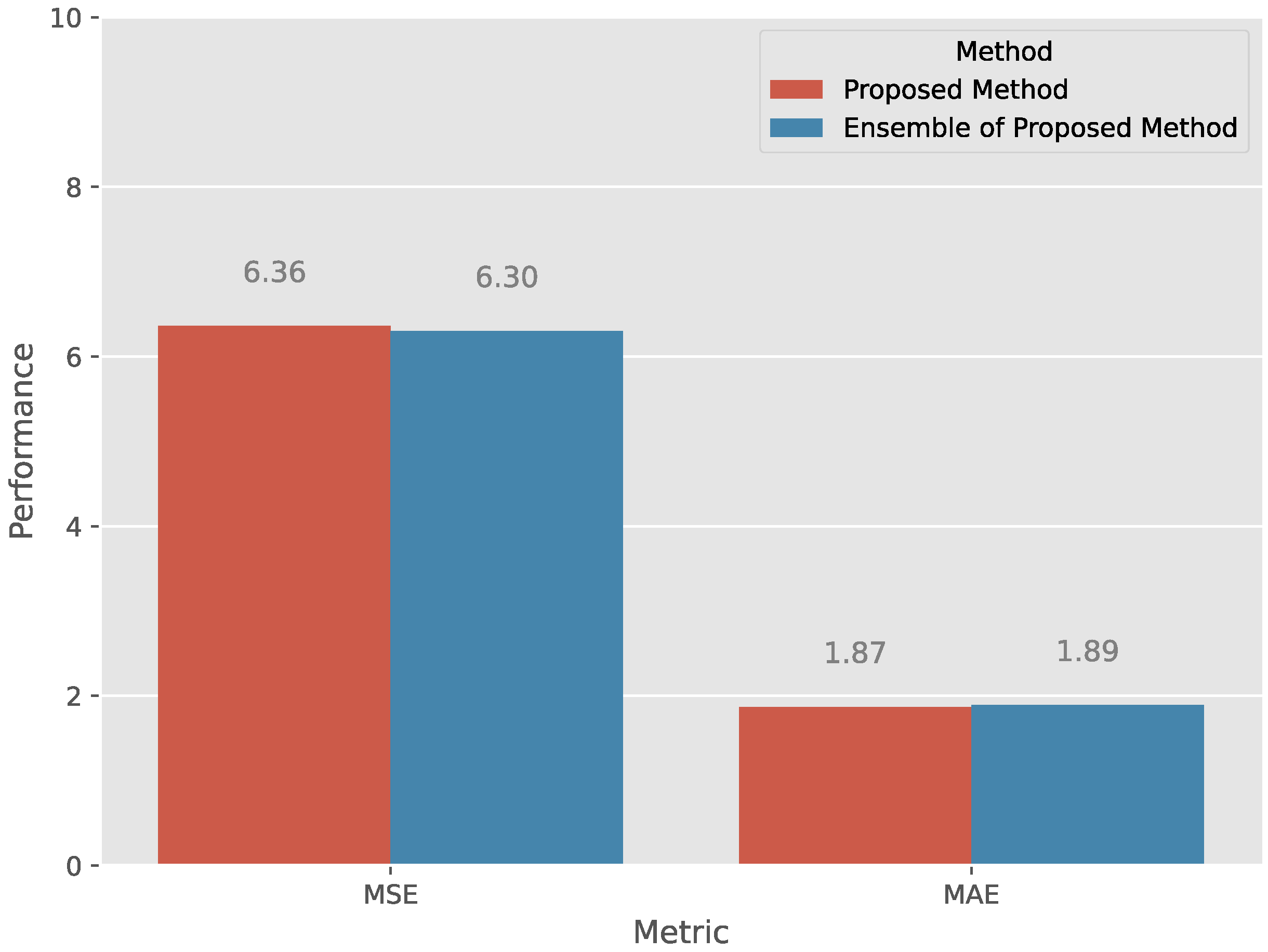
Ensemble learning is an important technique for model improvement and is also a widely used technique in data science competitions. Ensemble learning can be further divided into three categories, boosting, bagging, and stacking. In the comparison methods, the gradient boosting regressor and XGBoost models belong to the boosting category, random forest is a bagging method, and the work conducted by Di et al. used a stacking approach to combine several base models. This work conducted a simple experiment to explore whether the proposed method benefited from ensemble learning. For the ensemble of fusion networks, we used the training set to train ten fusion networks. For each test sample, the ten models had to make their predictions, and the final prediction outcome was simply the average of the ten predictions. It is apparent that this approach is very simple, but it is also one of the most commonly used techniques to combine multiple base models. We used the same architecture with random initialization weights to train the ten fusion networks, which means that each fusion network was slightly different from the others.

Figure 7 shows the experimental results measured by MSE and MAE, each of which is the average of ten experiments. It can be seen from the results that the ensemble of the fusion network still worked well but the performance difference between these two approaches was very minor. Thus, the proposed method did not benefit from a simple ensemble approach. We conclude that the main reason for the result is that the difference between the fusion networks in the ensemble was very minor. Note that ensemble learning tended to yield better results than the underlying base models when there was significant diversity among the base models. However, the diversity of the fusion networks in the ensemble model was expected to be minor, which is why a simple ensemble approach did not result in a significant performance improvement.

4.6. The Impact of Dropout Probability and Batch Normalization

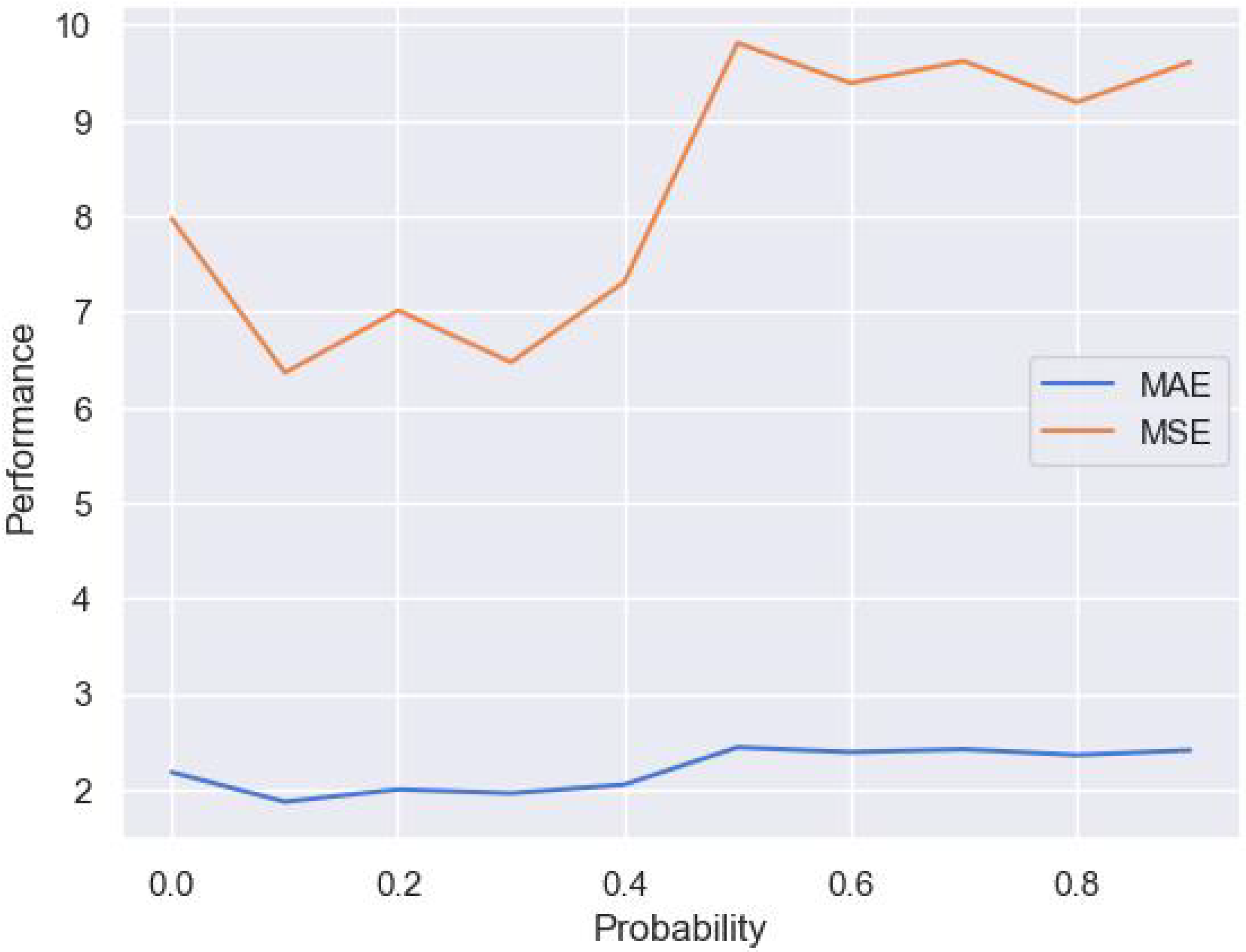
Dropout is a commonly used technique in deep learning to regularize and prevent the co-adaptation of neurons [37]. It can randomly zero some neurons in the layer with probability p, which is a hyperparameter. We performed a sensitivity analysis of p to investigate the performance impact caused by different values of p. We changed the value of p from 0 to 0.9, and each setting repeated the experiment ten times to avoid the randomness effect of the weight initialization. We used the average of ten experiments as the performance result. Figure 8 shows the experimental results. The model gave the best performance when p was 0.1 but the performance difference between the different settings was minor.

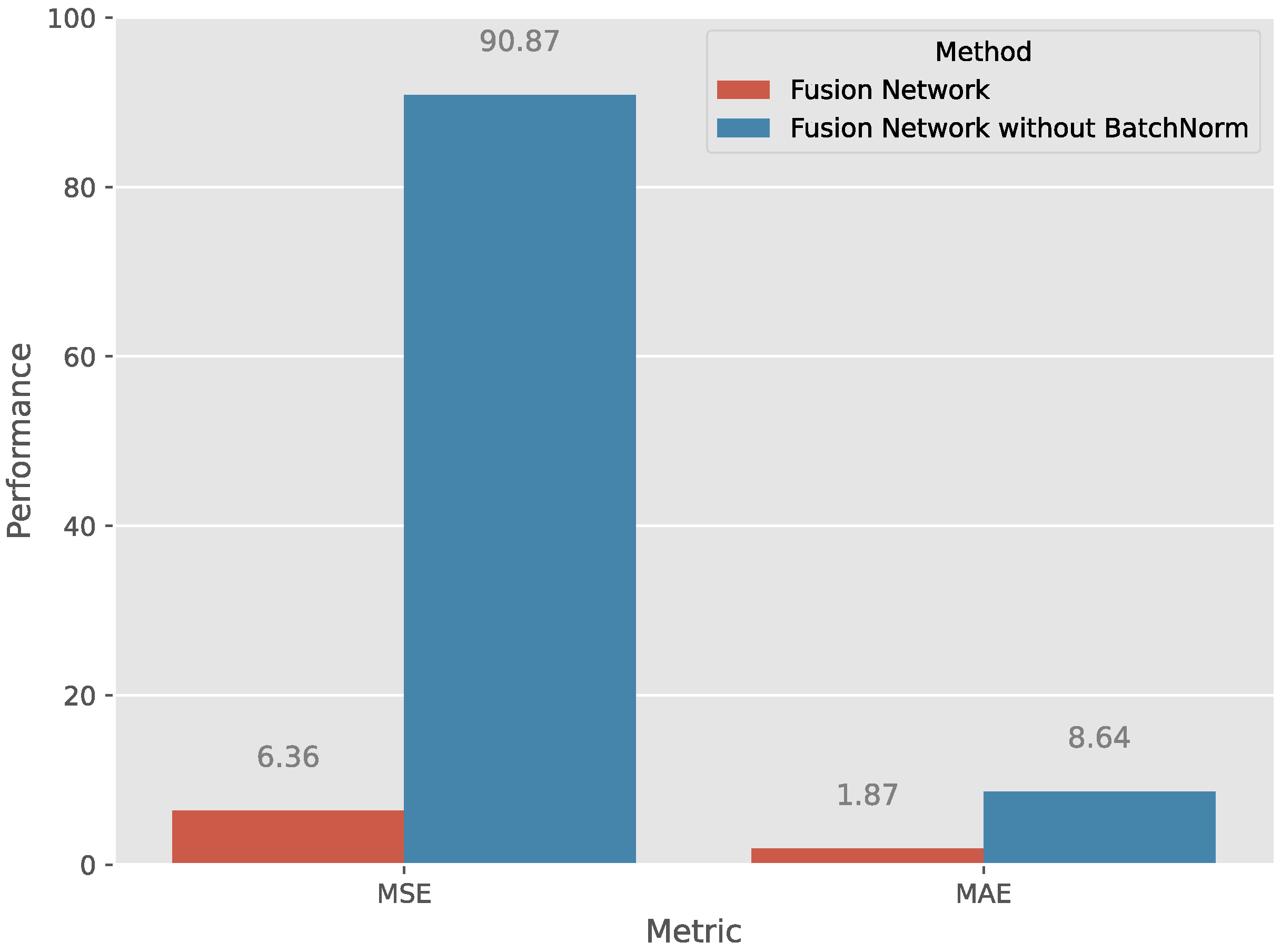
In addition to the dropout mechanism, batch normalization is another technique that can speed up model training, reduce the internal covariant shift, and regularize the model. We conducted experiments to explore the importance of batch normalization in our proposed model. Based on the previous experimental results, we set the dropout probability to 0.1 and designed a new model by removing all batch normalizations from the network. The experimental results measured by the MSE and MAE are listed in Figure 9, which indicated that batch normalization was an essential step in our proposed model. In contrast, the importance of the dropout was much less than that of batch normalization. These results also conform to the conclusions of the previous work [34], that is, the dropout can be removed or reduced in strength in a batch-normalized network.

5. Conclusions

In this work, we propose a deep learning model called a fusion network to predict the MRR. Central to our proposed model is the separation of the features into shallow and deep features, respectively, and the use of the characteristics of deep learning to perform a fusion of these two types of features. It is worth mentioning that the proposed method is flexible and can incorporate domain knowledge into the model. We conduct experiments on the PHM dataset and the experimental results indicate that the proposed model outperforms the winner of the 2016 PHM Data Challenge and three ensemble learning methods. In addition to the experimental results, a detailed analysis of the proposed method is also provided in this work. In one of our future works, we plan to identify new features based on the mechanism of CMP. Furthermore, it is worth applying our proposed method to other processing steps in semiconductor manufacturing.

References

1. Yang, W.T.; Blue, J.; Roussy, A.; Pinaton, J.; Reis, M.S. A Structure Data-Driven Framework for Virtual Metrology Modeling. IEEE Trans. Autom. Sci. Eng. 2019, 17, 1297–1306. [Google Scholar] [CrossRef]
2. Cho, Y.; Liu, P.; Jeon, S.; Lee, J.; Bae, S.; Hong, S.; Kim, Y.H.; Kim, T. Simulation and Experimental Investigation of the Radial Groove Effect on Slurry Flow in Oxide Chemical Mechanical Polishing. Appl. Sci. 2022, 12, 4339. [Google Scholar] [CrossRef]
3. Duan, Y.; Liu, M.; Dong, M.; Wu, C. A two-stage clustered multi-task learning method for operational optimization in chemical mechanical polishing. J. Process Control 2015, 35, 169–177. [Google Scholar] [CrossRef]
4. Zhao, Y.; Chang, L.; Kim, S. A mathematical model for chemical–mechanical polishing based on formation and removal of weakly bonded molecular species. Wear 2003, 254, 332–339. [Google Scholar] [CrossRef]
5. Jeong, S.; Jeong, K.; Choi, J.; Jeong, H. Analysis of correlation between pad temperature and asperity angle in chemical mechanical planarization. Appl. Sci. 2021, 11, 1507. [Google Scholar] [CrossRef]
6. Evans, C.J.; Paul, E.; Dornfeld, D.; Lucca, D.A.; Byrne, G.; Tricard, M.; Klocke, F.; Dambon, O.; Mullany, B.A. Material removal mechanisms in lapping and polishing. CIRP Ann. 2003, 52, 611–633. [Google Scholar] [CrossRef] [Green Version]
7. Qin, C.; Hu, Z.; Tang, A.; Yang, Z.; Luo, S. An efficient material removal rate prediction model for cemented carbide inserts chemical mechanical polishing. Wear 2020, 452, 203293. [Google Scholar] [CrossRef]
8. Park, S.; Lee, H. Electrolytically Ionized Abrasive-Free CMP (EAF-CMP) for Copper. Appl. Sci. 2021, 11, 7232. [Google Scholar] [CrossRef]
9. Son, J.; Lee, H. Contact-area-changeable CMP conditioning for enhancing pad lifetime. Appl. Sci. 2021, 11, 3521. [Google Scholar] [CrossRef]
10. Liu, H.; Wang, F.; Guo, D.; Liu, X.; Zhang, X.; Sun, F. Active Object Discovery and Localization Using Sound-Induced Attention. IEEE Trans. Ind. Inform. 2020, 17, 2021–2029. [Google Scholar] [CrossRef]
11. Wang, Y.G.; Zhang, L.C.; Biddut, A. Chemical effect on the material removal rate in the CMP of silicon wafers. Wear 2011, 270, 312–316. [Google Scholar] [CrossRef]
12. Jeng, Y.R.; Huang, P.Y. Impact of Abrasive Particles on the Material Removal Rate in CMP A Microcontact Perspective. Electrochem. Solid State Lett. 2004, 7, 40–43. [Google Scholar] [CrossRef]
13. Oliver, M.R.; Schmidt, R.E.; Robinson, M. CMP pad surface roughness and CMP removal rate. In Proceedings of the 198th Meeting of the Electrochemical Society, 4th International Symposium on CMP, Phoenix, AZ, USA, 23–25 October 2000; Volume 26, pp. 77–83. [Google Scholar]
14. Park, K.H.; Kim, H.J.; Chang, O.M.; Jeong, H.D. Effects of pad properties on material removal in chemical mechanical polishing. J. Mater. Process. Technol. 2007, 187, 73–76. [Google Scholar] [CrossRef]
15. Ng, W.X.; Chan, H.K.; Teo, W.K.; Chen, I.M. Programming a robot for conformance grinding of complex shapes by capturing the tacit knowledge of a skilled operator. IEEE Trans. Autom. Sci. Eng. 2015, 14, 1020–1030. [Google Scholar] [CrossRef]
16. Dambon, O.; Demmer, A.; Peters, J. Surface interactions in steel polishing for the precision tool making. CIRP Ann. 2006, 55, 609–612. [Google Scholar] [CrossRef]
17. Oh, S.; Seok, J. An integrated material removal model for silicon dioxide layers in chemical mechanical polishing processes. Wear 2009, 266, 839–849. [Google Scholar] [CrossRef]
18. Carvalho, T.P.; Soares, F.A.; Vita, R.; Francisco, R.d.P.; Basto, J.P.; Alcalá, S.G. A systematic literature review of machine learning methods applied to predictive maintenance. Comput. Ind. Eng. 2019, 137, 106024. [Google Scholar] [CrossRef]
19. Dinh, T.Q.; Marco, J.; Greenwood, D.; Ahn, K.K.; Yoon, J.I. Data-based predictive hybrid driven control for a class of imperfect networked systems. IEEE Trans. Ind. Inform. 2018, 14, 5187–5199. [Google Scholar] [CrossRef] [Green Version]
20. Wan, J.; Tang, S.; Li, D.; Wang, S.; Liu, C.; Abbas, H.; Vasilakos, A.V. A Manufacturing Big Data Solution for Active Preventive Maintenance. IEEE Trans. Ind. Inform. 2017, 13, 2039–2047. [Google Scholar] [CrossRef]
21. Ibrahim, A.; Eltawil, A.; Na, Y.; El-Tawil, S. A machine learning approach for structural health monitoring using noisy data sets. IEEE Trans. Autom. Sci. Eng. 2019, 17, 900–908. [Google Scholar] [CrossRef]
22. Purwins, H.; Barak, B.; Nagi, A.; Engel, R.; Höckele, U.; Kyek, A.; Cherla, S.; Lenz, B.; Pfeifer, G.; Weinzierl, K. Regression methods for virtual metrology of layer thickness in chemical vapor deposition. IEEE/ASME Trans. Mechatron. 2013, 19, 1–8. [Google Scholar] [CrossRef] [Green Version]
23. Kourti, T. Application of latent variable methods to process control and multivariate statistical process control in industry. Int. J. Adapt. Control Signal Process. 2005, 19, 213–246. [Google Scholar] [CrossRef]
24. Park, C.; Kim, Y.; Park, Y.; Kim, S.B. Multitask learning for virtual metrology in semiconductor manufacturing systems. Comput. Ind. Eng. 2018, 123, 209–219. [Google Scholar] [CrossRef]
25. Choi, J.E.; Hong, S.J. Machine learning-based virtual metrology on film thickness in amorphous carbon layer deposition process. Meas. Sensors 2021, 16, 100046. [Google Scholar] [CrossRef]
26. Hirai, T.; Kano, M. Adaptive Virtual Metrology Design for Semiconductor Dry Etching Process Through Locally Weighted Partial Least Squares. IEEE Trans. Semicond. Manuf. 2015, 28, 137–144. [Google Scholar] [CrossRef] [Green Version]
27. Tsai, J.; Chou, P.; Chou, J. Color Filter Polishing Optimization Using ANFIS With Sliding-Level Particle Swarm Optimizer. IEEE Trans. Syst. Man, Cybern. Syst. 2018, 50, 1193–1207. [Google Scholar] [CrossRef]
28. Di, Y.; Jia, X.; Lee, J. Enhanced virtual metrology on chemical mechanical planarization process using an integrated model and data-driven approach. Int. J. Progn. Health Manag. 2017, 8, 31. [Google Scholar] [CrossRef]
29. Wang, P.; Gao, R.X.; Yan, R. A deep learning-based approach to material removal rate prediction in polishing. CIRP Ann. 2017, 66, 429–432. [Google Scholar] [CrossRef]
30. Yu, T.; Li, Z.; Wu, D. Predictive modeling of material removal rate in chemical mechanical planarization with physics-informed machine learning. Wear 2019, 426, 1430–1438. [Google Scholar] [CrossRef]
31. Yang, B.; Liu, R.; Zio, E. Remaining useful life prediction based on a double-convolutional neural network architecture. IEEE Trans. Ind. Electron. 2019, 66, 9521–9530. [Google Scholar] [CrossRef]
32. Bottou, L. Large-scale machine learning with stochastic gradient descent. In Proceedings of the COMPSTAT’2010, Paris, France, 22–27 August 2010; Springer: Berlin/Heidelberg, Germany, 2010; pp. 177–186. [Google Scholar]
33. Ge, R.; Huang, F.; Jin, C.; Yuan, Y. Escaping from saddle points—Online stochastic gradient for tensor decomposition. In Proceedings of the Conference on Learning Theory, PMLR, Paris, France, 3–6 July 2015; pp. 797–842. [Google Scholar]
34. Ioffe, S.; Szegedy, C. Batch Normalization: Accelerating Deep Network Training by Reducing Internal Covariate Shift. In Proceedings of the 32nd International Conference on Machine Learning, PMLR, Lille, France, 6–11 July 2015. [Google Scholar]
35. Nair, V.; Hinton, G.E. Rectified Linear Units Improve Restricted Boltzmann Machines. In Proceedings of the 27th International Conference on Machine Learning, Haifa, Israel, 21–24 June 2010; Omnipress: Madison, WI, USA, 2010; pp. 807–814. [Google Scholar]
36. Krizhevsky, A.; Sutskever, I.; Hinton, G.E. Imagenet classification with deep convolutional neural networks. In Proceedings of the Advances in Neural Information Processing Systems, Lake Tahoe, NV, USA, 3–8 December 2012; pp. 1097–1105. [Google Scholar]
37. Srivastava, N.; Hinton, G.; Krizhevsky, A.; Sutskever, I.; Salakhutdinov, R. Dropout: A simple way to prevent neural networks from overfitting. J. Mach. Learn. Res. 2014, 15, 1929–1958. [Google Scholar]
38. Jia, X.; Di, Y.; Feng, J.; Yang, Q.; Dai, H.; Lee, J. Adaptive virtual metrology for semiconductor chemical mechanical planarization process using GMDH-type polynomial neural networks. J. Process Control 2018, 62, 44–54. [Google Scholar] [CrossRef]
39. Zhang, J.; Jiang, Y.; Luo, H.; Yin, S. Prediction of material removal rate in chemical mechanical polishing via residual convolutional neural network. Control Eng. Pract. 2021, 107, 104673. [Google Scholar] [CrossRef]
40. Chen, T.; Guestrin, C. Xgboost: A scalable tree boosting system. In Proceedings of the 22nd ACM Sigkdd International Conference on Knowledge Discovery and Data Mining, San Francisco, CA, USA, 13–17 August 2016; ACM: New York, NY, USA, 2016; pp. 785–794. [Google Scholar]
41. Ba, J.; Caruana, R. Do deep nets really need to be deep? In Proceedings of the Advances in Neural Information Processing Systems, Montreal, QC, Canada, 8–13 December 2014; Volume 27. [Google Scholar]
Figure 1. Data Analysis Flow.
Applsci 12 11478 g001
Figure 2. Removal Rate Distribution.
Applsci 12 11478 g002
Figure 3. Outlier Detection with Data Visualization.
Applsci 12 11478 g003
Figure 4. Fusion Network Architecture.
Applsci 12 11478 g004
Figure 5. The loss curves of our proposed model.
Applsci 12 11478 g005
Figure 6. Performance of different network architectures, where a lower value is better.
Applsci 12 11478 g006
Figure 7. Single fusion network vs. ensemble of fusion network, where a lower value is better.
Applsci 12 11478 g007
Figure 8. Results with different dropout probabilities.
Applsci 12 11478 g008
Figure 9. The impact of batch normalization, where a lower value is better.
Applsci 12 11478 g009