Abstract
Aerocapture maneuvers refer to a single atmospheric crossing to deplete orbital energy and establish a closed orbit. During the atmospheric flight, adjusting the spacecraft’s vertical lift component in an optimal manner, bang-bang bank control, will minimize the propulsion fuel consumption required to establish the target orbit. However, such methods have been suffering from the performance’s oversensitivity to the control’s instantaneous switching time and poor robustness. To address these problems, we propose a new numerical predictor-corrector guidance algorithm based on the saturation function profile in this paper. The saturation function is used to basically simulate the bang-bang control structure, which enhances the algorithm’s robustness by reducing its dependence on the relevant parameters without losing too much optimality. Monte Carlo simulations in both Earth and Mars scenarios demonstrate the robustness, accuracy, and near-optimal performance of the proposed guidance method.
1. Introduction
Aerocapture maneuvers make full use of the target planet’s atmospheric resources (mainly atmospheric drag) to reduce the spacecraft’s speed, and achieve the transfer from a hyperbolic orbit to an elliptical orbit through a single atmospheric crossing. Compared to orbit maneuvers that use only thrusters, aerocapture can save a lot of fuel, in return the spacecraft can carry more payloads to complete more scientific exploration missions. Since the concept of aerocapture was invented, much research [1,2,3,4,5,6,7] has been done to analyze and prove its feasibility and advantages in interplanetary flight and deep space exploration. Unlike aerobraking, which needs to pass through the atmosphere many times, aerocapture can greatly shorten the orbital transfer time, on the other hand the spacecraft needs to bear higher peak heat flow and the process is more dangerous. In addition, there’re significant uncertainties and disturbances involved in aerocapture maneuvers (i.e., variations in the atmospheric environment, aerodynamic coefficients, etc.), so a robust, reliable, and accurate guidance scheme is very necessary. At present, mainly two kinds of technologies have been developed in aerocapture guidance: trajectory tracking guidance and predictor-corrector guidance.
The trajectory tracking guidance, also named implicit guidance, attempts to track the preset reference trajectory [8]. Gurley [9] proposed an early Mars aerocapture tracking guidance method in 1993, which tracks the energy of the reference trajectory by adjusting the spacecraft’s pitch attitude. For the Mars 2001 mission, Ro et al. [10] developed a guidance algorithm based on the terminal-point controller (TPC). During aerocapture, the cosine of the bank angle is selected as the control variable to ensure that the spacecraft can fly near the predetermined optimal trajectory; finally, a suboptimal trajectory can be obtained. Rozanov and Guelman [11] changed the independent variable from time to specific mechanical energy, and tracked reference trajectory’s state space with variable structure control. This method does not need density estimation and can enhance the stability of guidance for specific tasks, but it has a great dependence on the nominal trajectory. If the actual environment changes greatly, the trajectory cannot be properly corrected and adjusted using this method, which will produce great errors. To enhance the robustness of the guidance, Kozynchenko [12] proposed a time-varying control method based on TPC, which controls the angle of attack and bank angle at the same time. The optimality obtained by the two-parameter time-varying control is found to be the same as that of the single-variable optimal control. The disadvantage is that the dynamic model used in [12] does not consider gravitational perturbation and the rotation of the atmosphere, so the guidance accuracy cannot be guaranteed. Zhang [13] and Han [14] applied the convex programming method to optimize the Mars aerocapture guidance. This method has the potential for real-time execution, but its effectiveness needs to be further verified. Yao et al. [15] implemented a novel integral sliding surface to avoid singularity, and the neural network is adopted to compensate for the lumped uncertain term, so the proposed tracking guidance law is robust against uncertainties.
The predictor-corrector guidance, also known as explicit guidance, repeatedly searches for the optimal or near-optimal path from the current state to the target state [8]. According to different ways of predicting terminal states, it can be divided into analytical predictor-corrector (APC) guidance and numerical predictor-corrector (NPC) guidance. Masciarelli et al. [16] discussed and tested two APC guidance methods, also known as the hybrid predictor-corrector aerocapture scheme (HYPAS), for aerocapture in Mars sampling return mission. Both algorithms are derived from the algorithm in the aerocapture flight test (AFE) [17]. Based on HYPAS, Chad Hanak et al. [18] proposed an improved bank angle control law for the exit phase in Mars and Titan aerocapture. Through feedback linearization, the gain that is difficult to solve analytically and needs to change with mission parameters is eliminated. The improved guidance algorithm performs well in the limited test of the Mars mission. However, for Titan’s aerocapture mission, which lacks a more accurate atmospheric model, severe atmospheric changes still bring problems to the algorithm. Hamel et al. [19] adopted two measures to improve the APC algorithm’s robustness. The first is to add an energy controller in the capture and exit phases so that the switch between phases has a certain adaptability. Second, collect atmospheric density data in the capture phase to redefine the density scale height, and apply it to the exit phase. The improved algorithm can increase the width of the corridor and improve adaptability. However, when spacecraft need to fly a wide range, there may be a large deviation of atmosphere between the capture phase and the exit phase. Based on the segmented variable ballistic coefficient, Peng et al. [20] proposed an analytical predictive guidance algorithm for single ballistic coefficient switching. The terminal velocity after ballistic coefficient switching can be obtained in real time through analytical calculation, and the adaptive control of the ballistic coefficient switching time is realized at the same time. DiCarlo [21] improved the Higgins’ numerical predictor-corrector guidance method (PredGuid) [22] by adding an energy controller in the gliding phase so that the algorithm can adapt to high-energy trajectory. Putnam et al. [23] varied the ballistic coefficient by changing the spacecraft reference area to modulate the trajectory using the NPC guidance method. Lu et al. [24,25,26] proposed an NPC guidance algorithm FNPAG (full numerical predictor-corrector aerocapture guidance) based on the research of aerocapture optimal control theory (the bank angle control profile required to minimize the velocity increment of orbit correction has a bang-bang structure) [27,28,29]. The whole process consists of two phases. In phase 1, the control profile is stepped, that is, the spacecraft is assumed to first fly at the specified minimum bank angle, then switch to the relatively large bank angle. Once the current time reaches the switching time, start phase 2, in which the bank angle is set to a constant value. Webb [30,31] applied FNPAG to three different spacecrafts and obtained good results. Based on Lu’s research, Cihan et al. [8] proposed a new APC guidance method. In the descending phase, guidance is open-loop, simultaneously, atmospheric parameters are measured and fitted by a third-order Fourier series so that the comprehensive effects of atmospheric density, aerodynamic coefficients, and spacecraft mass can be parameterized. Then in the ascending phase, closed-loop guidance is started. The analytical functions of atmospheric density and flight path angle are used to predict the velocity at atmospheric exit, so the target apogee altitude can be tracked. In the Earth aerocapture scenario, this APC guidance method’s performance is very similar to the FNPAG algorithm.
However, the advanced guidance methods mentioned above have the same shortcoming. That is, their performances are greatly affected by the selection of switching time from open-loop to closed-loop guidance, which degrades the methods’ robustness, especially under significant uncertainties and disturbances. Moreover, the guidance process in literature [8] requires a lot of prior information, resulting in weak adaptability of the algorithm.
To solve the above problems of parameter sensitivity and poor robustness by utilizing the saturation function’s characteristics, this paper presents a numerical predictor-corrector guidance method based on the saturation function profile, which can basically simulate the bang-bang control structure while reducing the dependence on an algorithm on the relevant parameters, so as to enhance the algorithm’s robustness. Through Monte Carlo simulation and comparison with existing advanced algorithms, the performance of the proposed algorithm is verified.
The following paper is organized as follows. In Section 2, the 3 degree-of-freedom (DOF) dynamic model during atmospheric flight is presented, and the impulsive Orbital Maneuvers, including single-impulse aerocapture maneuver and the two-impulse aerocapture maneuvers, are described briefly. In Section 3, based on the decoupling idea of longitudinal and lateral channels, the longitudinal and lateral guidance laws are introduced respectively, and the complete numerical predictor-corrector guidance’s architecture is given. In Section 4, Monte Carlo simulation and parameter influence analysis are carried out in both the Earth and Mars aerocapture scenarios to prove the robustness and efficiency of the proposed method. Finally, conclusions are drawn in Section 5.
2. Aerocapture Modeling and Maneuver Description
2.1. Three-DOF Dynamic Model
During aerocapture, without loss of generality, we can assume that the celestial body is an oblate sphere rotating with constant angular velocity , and its atmosphere is at rest with respect to the celestial body. Then the three-dimensional equations describing the motion of the spacecraft are
where r is the radial distance from the center of the celestial body to the spacecraft’s center of mass; and are longitude and latitude, respectively; V refers to the velocity of the spacecraft relative to the celestial body; is the flight path angle of the velocity vector relative to the celestial body; denotes the heading angle (turning clockwise from the due north, the projection of the relative velocity vector of the celestial body on the local horizontal plane is positive); refers to the bank angle, and are the gravitational acceleration’s radial and latitudinal components, respectively, which are calculated as follows,
where is the gravitational parameter of the celestial body, is the equatorial radius of the celestial body, and is the second zonal coefficient (for oblateness). In addition, the aerodynamic lift and drag accelerations (L and D) are conventionally defined as
where is the atmospheric density; S denotes the reference area of the spacecraft; , are lift coefficient and drag coefficient respectively; m is the mass of the spacecraft. In this work, the Martian atmosphere uses the atmospheric exponential model fitted according to the inflight measurement data of Viking-1 launched by NASA in 1976 as the nominal density model,
where, the reference density , the scale altitude , h is the altitude of the spacecraft. While the Earth’s atmosphere uses the 1976 U.S. standard atmosphere model as the nominal density model. The orbital maneuver above the celestial atmosphere is calculated by the spacecraft’s inertial velocity expressed in the equatorial inertial coordinate system. The inertial velocity vector is equal to the sum of the relative velocity vector and the cross product of the celestial body’s self-rotation angle velocity vector and the spacecraft’s position vector :
2.2. Impulsive Orbital Maneuvers
At the entry interface (EI), the spacecraft enters the atmosphere. After atmospheric flight and energy dissipation, the spacecraft exits the atmosphere. Then in the exo-atmospheric flight phase, one or two impulse maneuvers are required to establish the desired target orbit. Figure 1 shows the complete single-impulse aerocapture maneuver. In this case, the apogee radius of post-atmospheric flight is equal to the radius of the apogee of the target orbit. The single velocity increment required to establish the target orbit is
where , are the apogee radius and perigee radius of the target orbit, respectively, and for a single-impulse maneuver, ; , are the apogee and perigee radii of the orbit after aerocapture, which are determined by the following formulas:
where a is the semi-major axis of the orbit after aerocapture, , , and are the radius, inertial velocity, and flight path angle, respectively, at the atmospheric exit. In addition, a is determined by the kinetic energy and potential energy at the atmospheric exit:
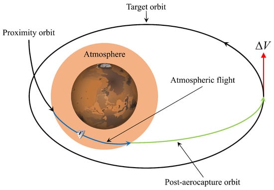
Figure 1.
Single-impulse aerocapture maneuver, .
On the other hand, when the post-aerocapture orbit’s apogee radius does not match that of the target orbit, it is necessary to carry out a two-impulse maneuver to establish the target orbit. Figure 2 shows the situation that the apogee of the post-aerocapture orbit is lower and higher than that of the target orbit, respectively, where the first impulse (collinear with the velocity at the apogee) raises the apogee to the desired altitude, then after flying half an ellipse, the second impulse raises or lowers the new perigee to the target orbit. The required total velocity increment of the two impulses is
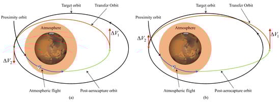
Figure 2.
Two-impulse aerocapture maneuver: (a) ; (b) .
If the target orbit is a circular orbit, that is, , then the above formula can be simplified as
3. Guidance Law Design Based on Saturation Function
3.1. Longitudinal Guidance Law
The main goal of the longitudinal guidance law of aerocapture is to determine the magnitude of the bank angle to minimize the orbital insertion’s velocity increment after the atmospheric flight. To reduce the algorithm’s complexity and make it possible to be applied online, the main control variable of the trajectory to be designed is the bank angle , while the angle of attack follows a predetermined profile considering trim flight, thermal protection system, and so on [24].
According to Lu [24], when lateral control is ignored in aerocapture (i.e., there is no constraint on the final orbit inclination), the two-phase bank angle control with bang-bang structure can achieve the minimum ,
where t is the current time; is a selected small bank angle magnitude used in the first phase; is a relatively large bank angle magnitude used in the second phase; denotes the switching time from to . However, the guidance performance of this control profile is very sensitive to the selection of the switching time. To reduce the sensitivity to the corresponding parameter without losing too much optimality, a guidance profile based on the saturation function is proposed for predictor-corrector guidance. Firstly, the saturation function is introduced,
where denotes the time when the corresponding saturation function reaches the median, and it’s the guidance parameter that must be determined; can be preset as a constant value. Considering that the value range of is [−1, 1], let and denote the upper and lower bounds of bank angle magnitude, respectively, then the control profile based on can be written as
At the same time, a linear function is introduced to prevent premature saturation of bank control so that the guidance law can have more control margin to cope with uncertainties and disturbances,
where , can be preset as constant values. The final specific guidance profile is
The proposed guidance profile has mainly three advantages. First, it is similar to the optimal bang-bang control due to the introduction of saturation function, so the guidance method based on this profile can realize near-optimal performance. Second, different from the instantaneous and discontinuous switching in the bang-bang profile, the control magnitude’s switching in this profile based on saturation function is smoother and easier to adjust, which is conducive to reducing the aforementioned parameter sensitivity and improving the guidance method’s robustness. Third, compared with the aforementioned two-phase guidance scheme, the proposed guidance profile can be applied to the whole phase of aerocapture, making the guidance process more unified and continuous.
In each guidance cycle, after the determination of , the complete bank angle magnitude profile can be defined by the above equation. Under the control of this profile, the state at atmospheric exit is obtained by numerical integration of the differential equations of motion, and then the post-aerocapture orbit and the velocity increment required for orbital insertion are determined by Equations (13)–(18). After that, we can correct according to the deviation between the prediction and the target. In the light of different maneuvering modes, single-impulse maneuvering requires that the post-aerocapture orbit apogee coincides with the target apogee, so it is a single parameter root seeking problem, which can be solved by false position method; The two-impulse maneuver is to minimize total velocity increment, so it is a single-parameter optimization problem, which can be solved by fminbnd function in MATLAB. Considering the problem’s complexity, an effective initial guess method is adopted, that is, select the converged solution obtained from the previous guidance period as the initial value. This method will significantly improve the convergence speed of solving . While the symbol of is determined by the lateral logic introduced in the following sections. Whenever the bank reversal is required, the guidance system will directly change the symbol of the bank angle.
3.2. Lateral Guidance Law
Unlike the longitudinal motion, which determines the orbital shape, the lateral motion mainly determines the direction of orbital angular momentum, which is reflected in the orbital inclination i. This paper adopts a predictive single bank reversal logic: in each guidance cycle, we assume that the bank angle is reversed at the current time, then run the predictive guidance scheme (as mentioned above), and obtain the post-aerocapture orbit inclination . If is equal to the expected orbit inclination or meets the accuracy requirements,
then we reverse the bank angle. It should be noted that the bank angle rate and acceleration limits are applied to the numerical integration process and ensure that the spacecraft rolls along the shortest path to reduce the impact on longitudinal motion.
Moreover, as a model-based algorithm, the uncertainty of aerodynamic coefficients ( and ), atmospheric density, and vehicle mass will significantly affect the performance of the aerocapture guidance algorithm [32]. If the estimated information of aerodynamic coefficients and atmospheric density deviation can be used reasonably, the algorithm will achieve the desired high guidance accuracy, especially when the aerocapture process is under severe uncertainties and disturbances. Therefore, it is necessary for the guidance system to make appropriate online corrections according to the aerodynamic parameters measured in real time.
Aerocapture’s dispersions include the dispersions of entry states, aerodynamics, spacecraft mass, and atmospheric density. Except for the dispersions of entry states, all dispersion only affects the spacecraft’s lift and drag accelerations. During flight, the actual values of lift and drag accelerations can be calculated from navigation data and accelerometer output. In the absence of other measurement means (such as the accurate measurement system of atmospheric data), it is impossible to distinguish the influence of a dispersion source (such as density) from others (such as aerodynamic coefficients). However, it needs only to estimate the comprehensive effect of these dispersions. Therefore, a simple first-order low-pass filter can be used to estimate the dispersion effect and smooth the measured data:
where is the ratio of the current measured value (lift or drag acceleration) to the corresponding nominal value obtained from the nominal model, is the filter ratio of the last guidance cycle, and is a gain in the range (0, 1). The larger the gain, the better the filter’s smoothness, but the lower the sensitivity; Otherwise, the sensitivity is higher, but the stability is worse. Generally, a value slightly less than 1 is taken so that the impact of the previous round of filtration ratio on the current filtration ratio is greater. In this paper, , and the sampling time of the filter can be equal to the guidance period.
When initializing the filter, is set to 1. In each guidance cycle, the filter’s output is multiplied by the nominal lift L (or drag D) profile, and the subsequent trajectory is calculated based on the corrected profile.
3.3. Architecture of the Numerical Predictor-Corrector Guidance
Based on the guidance law in the two channels mentioned above, the whole predictor-corrector guidance procedure for aerocapture is shown in Figure 3. At the beginning of a guidance cycle, based on the spacecraft’s current states and guidance profile, the longitudinal guidance law predicts the atmospheric exit state by numerically integrating the three-DOF dynamic equations. Then we can calculate the post-aerocapture orbit parameters and total velocity increment required to perform orbit insertion. If the orbit parameters and don’t meet the mission requirements, we will correct the guidance parameter and update the guidance profile. The longitudinal guidance system repeats the above process until the mission requirements are met, then the bank-angle magnitude is determined. As for the lateral channel, the lateral guidance law determines the bank-angle symbol by judging if the post-reversal orbit inclination satisfies the mission requirement. Combining the outputs of both two channels, we can get the bank-angle command in the current guidance cycle. According to the bank-angle command, we update the spacecraft’s states through measurement in actual flight or integration of the dynamics Equations (1)–(6) in simulation. Then, the first-order low-pass filter is used to estimate the dispersion effect and update the aerodynamic profile. After that, we repeat the above steps in the next guidance cycle.
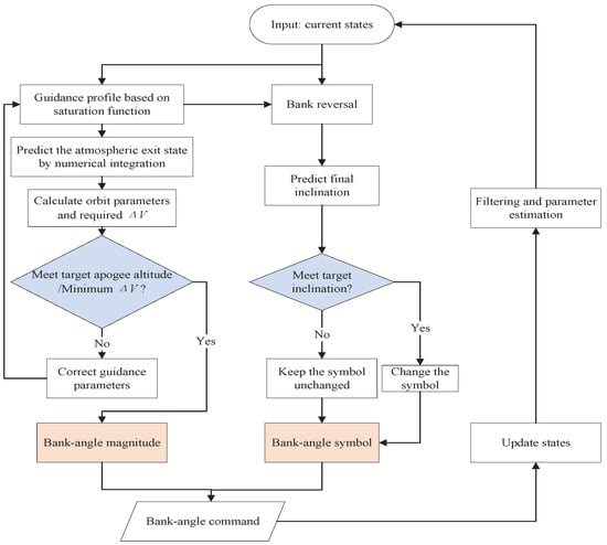
Figure 3.
Architecture of the predictor-corrector guidance procedure.
4. Simulations and Result Analysis
In this section, Monte Carlo simulation is used to test the performance and robustness of the proposed aerocapture guidance algorithm. In the simulation, we select the Orion multipurpose crew vehicle (MPCV) as the spacecraft model, including the spacecraft mass , reference area . Considering that the spacecraft flies at a high Mach number in an aerocapture scenario, and the aerodynamic coefficients hardly change at very high velocity, we can set the coefficients as constants during aerocapture [33,34]. Therefore, drag coefficient , lift-to-drag ratio , bank angle rate limit , and bank angle acceleration limit [24,35].
With the accelerating process of human exploration of the moon and Mars, the energy-saving capture at the Moon-Earth return and Mars has become a research hotspot [36,37,38]. Therefore, to fully test and verify the proposed algorithm’s performance, simulations will be carried out in two scenarios: Earth and Mars. Table 1 shows the nominal entry initial state under the two scenarios [15,35]. In the Earth scenario, the target orbit is a circular orbit with an altitude of 200 km and an inclination of 89 deg; In the Mars scenario, the target orbit is an elliptical orbit with an apogee altitude of 3000 km, a perigee altitude of 300 km, and an inclination of 89 deg.

Table 1.
Nominal inertial entry conditions.
4.1. Algorithm Verification and Analysis
In the Earth’s aerocapture scenario, we first conduct simulations regardless of parameter dispersions. The nominal results are shown in Figure 4, from which we can see that the spacecraft’s velocity decreases from 11,000 m/s to about 7800 m/s through aerocapture, and the bank angle basically follows a saturation function profile. In addition, there is a bank reversal in about 200 s. The required total is 64.67 m/s for this case, and the target apoapsis altitude and orbit inclination are well met. Based on the nominal results, we can further verify the method’s performance by Monte Carlo simulation.
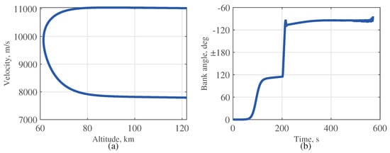
Figure 4.
Nominal results for Earth aerocapture: (a) relative velocity versus altitude; (b) bank angle versus time.
4.1.1. Preliminary Monte Carlo Simulation
The Monte Carlo simulation considers random changes in the entry state, vehicle mass, aerodynamic coefficients, and atmospheric density. Table 2 and Table 3 show the dispersions in the entry state and spacecraft parameters. Only the spacecraft’s mass follows a uniform distribution, others follow a Gaussian distribution. Note that the mean value of all random variables is zero. Compared with literature [35], dispersions of entry state have doubled in this paper, and the lift and drag coefficients’ 3 dispersions also increase from 15% to 20%.
Table 2.
Entry-state dispersions for the Monte Carlo simulation.
Table 3.
Vehicle parameter dispersions for the Monte Carlo simulation.
Regarding atmospheric density dispersions, ideally, they can be modeled by the Earth Global Reference Atmospheric Model (GRAM) [39]. Without access to it, a simplified analytical model of atmospheric density is used to simulate the dispersion characteristics,
where is the nominal atmospheric density, is a constant bias subject to a uniform distribution, and are amplitudes subject to a uniform distribution, and are parameters representing low and high frequencies, respectively, which reflect the disturbances’ periodic changes in altitude, and is the phase.
Based on the above dispersions, 100 Monte Carlo simulations are carried out in the Earth aerocapture scenario, and the simulation results are shown in Figure 5 and Figure 6. Figure 5 shows the relationship between relative velocity and altitude. It can be seen that the decrease in velocity, that is, energy dissipation, mainly occurs in a narrow 15 km altitude zone from 60 to 75 km. In addition, the exit velocities are all between 7750 and 7850 m/s. In Figure 6, the bank angle control profile for Monte Carlo simulations is shown. It can be seen that the bank angle time history basically conforms to the bang-bang structure, ensuring the algorithm’s near-optimal performance. In most of the simulations, the bank reversal happens in about 200 s. Due to various parametric disturbances, the bank angle in some cases finally saturates, while in others, it remains within a certain range.
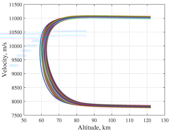
Figure 5.
Relative velocity versus altitude for Earth aerocapture.
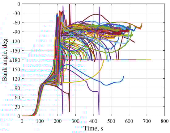
Figure 6.
Bank angle versus time for Earth aerocapture.
To further verify the algorithm’s performance through comparison, the method proposed in this article is designated as Mode 1, and the single-impulse guidance method proposed in the literature [24] is designated as Mode 2. Monte Carlo simulation is carried out under the same conditions, including the same scenario, spacecraft model, entry conditions, dispersions, and operational limits. The statistical results are shown in Table 4. From the table, the total ’s mean value and standard deviation in Mode 1 are smaller than those in Mode 2. The total ’s mean value in Mode 1 is reduced by 42.5% compared to that in Mode 2. Moreover, under the lateral guidance law, single bank reversal can make the spacecraft’s final inclination reach the target value. Therefore, the guidance requirements are well met in Mode 1, and Mode 1 performs better in optimality and robustness through the comparison.
Table 4.
Statistical results from Monte Carlo simulations for Earth aerocapture.
4.1.2. Parameter Impact Analysis and Comparison
To further test the method under more rigorous conditions, we vary the entry flight path angle and the spacecraft’s lift-to-drag ratio in a wider range, and analyze their impacts on the performance of the guidance algorithm.
Set the dispersion of the entry flight path angle to be uniformly distributed in [−0.5, 0.5] deg, and 1000 Monte Carlo simulations are carried out in the Earth scenario. The guidance results of the method proposed in this paper (Mode 1) and the method in the literature [24] (Mode 2) are shown in Figure 7. Through comparison, it can be clearly seen that when goes very steeper or very shallower, increases significantly in both Mode 1 and Mode 2. Under the large variation of entry flight path angle, the minimum value of obtained in Mode 1 is basically equal to that in Mode 2, indicating near-optimal performance. Moreover, the ’s dispersion in Mode 1 is smaller, and the standard deviation is reduced by 40.7% compared to that of mode 2. Furthermore, there is no extreme value of exceeding 400 m/s in Mode 1, which also shows that our method is more adaptive to the variation of entry flight path angle.
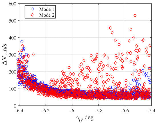
Figure 7.
Dispersion of the velocity increments with the different initial flight path angles for Earth aerocapture.
Then we study the impact of the lift-to-drag ratio on the performance of the guidance algorithm. The comparison results of 1000 Monte Carlo simulations in the Earth scenario are shown in Figure 8. It can be seen that although the in both Mode 1 and Mode 2 increases significantly at the very low lift-to-drag ratio, the in Mode 1 can still maintain a relatively small value at a very high lift-to-drag ratio. In addition, the standard deviation in Mode 1 is reduced by 51.1% compared with that in Mode 2, which proves our method’s good robustness.
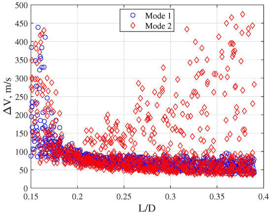
Figure 8.
Dispersion of the velocity increments with the different lift-to-drag ratios for Earth aerocapture.
4.2. Mars Aerocapture Mission
For the Mars aerocapture mission, we start with the simulations in a nominal case. The nominal results are shown in Figure 9. It can be seen that the spacecraft’s velocity drops from 5900 m/s to about 3900 m/s through aerocapture. The bank angle initially changes approximately in the form of a saturation function. However, due to Mars’ thin atmosphere, the bank angle eventually saturates to 0 to provide sufficient upward lift. The bank reversal happens in about 230 s. In this case, the required total is 54.47 m/s, and the target apoapsis altitude and orbit inclination are well met. Based on the nominal results, we further test the method’s performance through Monte Carlo simulation.
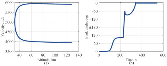
Figure 9.
Nominal results for Mars aerocapture: (a) relative velocity versus altitude; (b) bank angle versus time.
4.2.1. Preliminary Monte Carlo Simulation
Based on the dispersions mentioned above, 100 Monte Carlo simulations are carried out in the Mars scenario, and the simulation results are shown in Figure 10 and Figure 11.
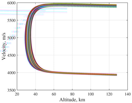
Figure 10.
Relative velocity versus altitude for Mars aerocapture.
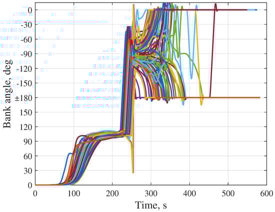
Figure 11.
Bank angle versus time for Mars aerocapture.
Figure 10 shows the relative velocity versus altitude. It can be seen that the velocity decreases mainly in a narrow 20 km altitude zone between 30 and 50 km, and finally, the exit velocity is between 3900 and 4000 m/s. Figure 11 shows the bank angle time histories of the Monte Carlo simulation. From this figure, the bank angle’s variation basically follows the bang-bang structure, which ensures the algorithm’s near-optimal performance. The bank angle is reversed at about 230 s, and then in some cases, it finally saturates to 180 deg, while in others, it saturates to 0 due to various parametric disturbances and inaccuracies in propagating the roll dynamics.
Similarly to the simulation in the Earth scenario, the simulation statistical results in Mode 1 and Mode 2 for the Mars aerocapture can be obtained, as shown in Table 5. Through comparison, it can be seen that the total ’s mean value and standard deviation obtained by our method are smaller, and the mean value of in Mode 1 is reduced by 8.0% compared to that of Mode 2, indicating that our method performs better in optimality and robustness. In addition, the final deviation from the target orbit inclination is small, ensuring that the guidance requirements can be well met.
Table 5.
Statistical results from Monte Carlo simulations for Mars aerocapture.
4.2.2. Parameter Impact Analysis and Comparison
Similarly, the impacts of entry flight path angle and the spacecraft’s lift-to-drag ratio on the guidance algorithm’s performance are studied.
Consider that the dispersion of the entry flight path angle is uniformly distributed on [−0.5, 0.5] deg, and 1000 Monte Carlo simulations are carried out in the Mars scenario. The guidance results of Mode 1 and Mode 2 are shown in Figure 12. It can be seen that both two guidance algorithms can adapt to a wide range of variation in entry flight path angle, but the velocity increment’s dispersion obtained in Mode 1 is significantly smaller. Given that the ’s standard deviation in Mode 1 is reduced by 53.6% compared with that in Mode 2, the method proposed in this paper has better robustness.
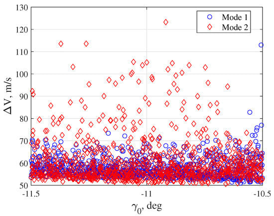
Figure 12.
Dispersion of the velocity increments with the different lift-to-drag ratios for Mars aerocapture.
The Monte Carlo simulation results that vary the lift-to-drag ratio in the Mars scenario are shown in Figure 13. Through comparison, the velocity increment does not change significantly with the large-scale variation of the lift-to-drag ratio in both Mode 1 and Mode 2, but its dispersion obtained by the method proposed in this paper is significantly smaller. The standard deviation of the velocity increment in Mode 1 is reduced by 66.4% compared with that in Mode 2, indicating the proposed method’s better performance.
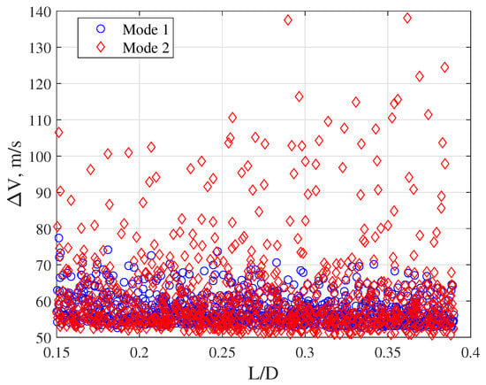
Figure 13.
The dispersion of the velocity increases with different lift-to-drag ratios for the Mars aerocapture.
From the simulation results in the Earth scenario and the Mars scenario, we can see that the guidance algorithm proposed in this paper not only ensures near-optimal performance, but also has better robustness than the comparison algorithm. Furthermore, the guidance performance of our method is relatively less affected by the large-scale variations of entry flight path angle and lift-to-drag ratio, indicating strong adaptability.
5. Conclusions
In this paper, focusing on the long-standing switching time sensitivity of the optimal aerocapture bang-bang control structure, a new numerical predictor-corrector aerocapture guidance scheme based on the profile of the saturation function is proposed. By replacing the previous instantaneous switching segmented guidance structure with saturation function, the method performance’s dependence on the switching time and other related parameters is reduced. Furthermore, the whole aerocapture guidance process is more unified without losing more optimality. Taking into account parameter uncertainties, disturbances, and operational constraints, the corresponding strategies are implemented. A large number of Monte Carlo simulations in Earth and Mars aerocapture scenarios show that the guidance method proposed in this paper is robust and accurate, which effectively alleviates the problem that a small error in switching time will lead to a significant error in exit state. Compared to the most advanced numerical predictor-corrector guidance scheme, it provides near-optimal performance and improved robustness. At the same time, the performance index’s dispersion is smaller under various disturbances. The parameter impact analysis shows that the proposed guidance method can adapt well to large-scale variations in the angle of the entry flight path and the lift-to-drag ratio. Based on these analyses, this new numerical predictor-corrector algorithm should be a feasible guide choice for future aerocapture missions.
Author Contributions
Conceptualization, J.C. and H.H.; methodology, J.C. and T.Q.; software, J.C. and R.T.; validation, J.C. and T.Q.; formal analysis, J.C.; investigation, R.T. and T.Q.; resources, H.H. and T.Q.; data curation, J.C. and R.T.; writing—original draft preparation, J.C.; writing—review and editing, H.H., R.T. and T.Q.; visualization, J.C. and R.T.; supervision, H.H. and T.Q.; project administration, H.H.; funding acquisition, H.H. All authors have read and agreed to the published version of the manuscript.
Funding
This research was funded by the National Natural Science Foundation of China, under Grant No. U20B2001 and Beijing Institute of Technology Research Fund Program for Young Scholars (XSQD-2 2060303).
Institutional Review Board Statement
Not applicable.
Informed Consent Statement
Not applicable.
Data Availability Statement
Not applicable.
Acknowledgments
The authors thank the colleagues for their constructive suggestions and research assistance throughout this study.
Conflicts of Interest
The authors declare no conflict of interest.
References
- Hoffman, S. A comparison of aerobraking and aerocapture vehicles for interplanetary missions. In Proceedings of the Astrodynamics Conference, Seattle, WA, USA, 22–25 August 1984; American Institute of Aeronautics and Astronautics: Reston, VA, USA, 1984. [Google Scholar] [CrossRef]
- Hall, J.L.; Noca, M.A.; Bailey, R.W. Cost-Benefit Analysis of the Aerocapture Mission Set. J. Spacecr. Rocket. 2005, 42, 309–320. [Google Scholar] [CrossRef]
- Lockwood, M.K. Titan Aerocapture Systems Analysis. In Proceedings of the 39th AIAA/ASME/SAE/ASEE Joint Propulsion Conference and Exhibit, Huntsville, AL, USA, 20–23 July 2003; American Institute of Aeronautics and Astronautics: Reston, VA, USA, 2003. [Google Scholar] [CrossRef]
- Way, D.; Powell, R.; Masciarelli, J.; Starr, B.; Edquist, K. Aerocapture Simulation and Performance for the Titan Explorer Mission. In Proceedings of the 39th AIAA/ASME/SAE/ASEE Joint Propulsion Conference and Exhibit, Huntsville, AL, USA, 20–23 July 2003; American Institute of Aeronautics and Astronautics: Reston, VA, USA, 2003. [Google Scholar] [CrossRef]
- Munk, M.M.; Moon, S.A. Aerocapture Technology Development Overview. In Proceedings of the 2008 IEEE Aerospace Conference, Big Sky, MT, USA, 1–8 March 2008. [Google Scholar] [CrossRef]
- Spilker, T.R.; Adler, M.; Arora, N.; Beauchamp, P.M.; Cutts, J.A.; Munk, M.M.; Powell, R.W.; Braun, R.D.; Wercinski, P.F. Qualitative Assessment of Aerocapture and Applications to Future Missions. J. Spacecr. Rocket. 2019, 56, 536–545. [Google Scholar] [CrossRef]
- Austin, A.; Afonso, G. Enabling and Enhancing Science Exploration Across the Solar System: Aerocapture Technology for SmallSat to Flagship Missions. Bull. Am. Astron. Soc. 2021, 54, 1–8. [Google Scholar]
- Cihan, I.H.; Kluever, C.A. Analytical Earth-Aerocapture Guidance with Near-Optimal Performance. J. Guid. Control. Dyn. 2021, 44, 45–56. [Google Scholar] [CrossRef]
- Gurley, J.G. Guidance for an aerocapture maneuver. J. Guid. Control. Dyn. 1993, 16, 505–510. [Google Scholar] [CrossRef]
- Ro, T.; Queen, E. Study of martian aerocapture terminal point guidance. In Proceedings of the 23rd Atmospheric Flight Mechanics Conference, Snowmass, CO, USA, 10–12 August 1998; p. 4571. [Google Scholar]
- Rozanov, M.; Guelman, M. Aeroassisted orbital maneuvering with variable structure control. Acta Astronaut. 2008, 62, 9–17. [Google Scholar] [CrossRef]
- Kozynchenko, A.I. Development of optimal and robust predictive guidance technique for Mars aerocapture. Aerosp. Sci. Technol. 2013, 30, 150–162. [Google Scholar] [CrossRef]
- Zhang, S.J.; Açikmeşe, B.; Swei, S.S.M.; Prabhu, D. Convex programming approach to real-time trajectory optimization for Mars aerocapture. In Proceedings of the 2015 IEEE Aerospace Conference, Big Sky, MT, USA, 7–14 March 2015; pp. 1–7. [Google Scholar]
- Han, H.; Qiao, D.; Chen, H.; Li, X. Rapid planning for aerocapture trajectory via convex optimization. Aerosp. Sci. Technol. 2019, 84, 763–775. [Google Scholar] [CrossRef]
- Yao, Q.; Han, H.; Qiao, D. Nonsingular Fixed-Time Tracking Guidance for Mars Aerocapture with Neural Compensation. IEEE Trans. Aerosp. Electron. Syst. 2022, 58, 3686–3696. [Google Scholar] [CrossRef]
- Masciarelli, J.; Rousseau, S.; Fraysse, H.; Perot, E. An analytic aerocapture guidance algorithm for the Mars Sample Return Orbiter. In Proceedings of the Atmospheric Flight Mechanics Conference. American Institute of Aeronautics and Astronautics, Denver, CO, USA, 14–17 August 2000. [Google Scholar] [CrossRef]
- Cerimele, C.; Gamble, J. A simplified guidance algorithm for lifting aeroassist orbital transfer vehicles. In Proceedings of the 23rd Aerospace Sciences Meeting, Reno, NV, USA, 14–17 January 1985; American Institute of Aeronautics and Astronautics: Reston, VA, USA, 1985. [Google Scholar] [CrossRef]
- Hanak, C.; Crain, T.; Masciarelli, J. Revised Algorithm for Analytic Predictor-Corrector Aerocapture Guidance: Exit Phase. In Proceedings of the AIAA Guidance, Navigation, and Control Conference and Exhibit. American Institute of Aeronautics and Astronautics, Austin, TX, USA, 11–14 August 2003. [Google Scholar] [CrossRef]
- Hamel, J.F.; de Lafontaine, J. Improvement to the Analytical Predictor-Corrector Guidance Algorithm Applied to Mars Aerocapture. J. Guid. Control. Dyn. 2006, 29, 1019–1022. [Google Scholar] [CrossRef]
- Peng, Y.; Xu, B.; Lu, X.; Fang, B.; Zhang, H. Analytical Predictive Guidance Algorithm Based on Single Ballistic Coefficient Switching for Mars Aerocapture. Int. J. Aerosp. Eng. 2019, 2019, 5765901. [Google Scholar] [CrossRef]
- DiCarlo, J.L. Aerocapture Guidance Methods for High Energy Trajectories. Ph.D. Thesis, Massachusetts Institute of Technology, Cambridge, MA, USA, 2003. [Google Scholar]
- Gamble, J.; Cerimele, C.; Moore, T.; Higgins, J. Atmospheric guidance concepts for an aeroassist flight experiment. J. Astronaut. Sci. 1988, 36, 45–71. [Google Scholar]
- Putnam, Z.R.; Braun, R.D. Drag-modulation flight-control system options for planetary aerocapture. J. Spacecr. Rocket. 2014, 51, 139–150. [Google Scholar] [CrossRef]
- Lu, P.; Cerimele, C.J.; Tigges, M.A.; Matz, D.A. Optimal aerocapture guidance. J. Guid. Control Dyn. 2015, 38, 553–565. [Google Scholar] [CrossRef]
- Lu, P.; Brunner, C.W.; Stachowiak, S.J.; Mendeck, G.F.; Tigges, M.A.; Cerimele, C.J. Verification of a fully numerical entry guidance algorithm. J. Guid. Control Dyn. 2017, 40, 230–247. [Google Scholar] [CrossRef]
- Matz, D.A.; Lu, P.; Mendeck, G.F.; Sostaric, R.R. Application of a fully numerical guidance to Mars aerocapture. In Proceedings of the AIAA Guidance, Navigation, and Control Conference, Grapevine, TX, USA, 9–13 January 2017; p. 1901. [Google Scholar]
- Miele, A.; Wang, T.; Lee, W.; Zhao, Z. Optimal trajectories for the aeroassisted flight experiment. Acta Astronaut. 1990, 21, 735–747. [Google Scholar] [CrossRef]
- Han, H.; Qiao, D.; Chen, H. Optimal ballistic coefficient control for Mars aerocapture. In Proceedings of the 2016 IEEE Chinese Guidance, Navigation and Control Conference (CGNCC), Nanjing, China, 12–14 August 2016; pp. 2175–2180. [Google Scholar]
- Zhang, G.; Wen, C.; Han, H.; Qiao, D. Aerocapture Trajectory Planning Using Hierarchical Differential Dynamic Programming. J. Spacecr. Rocket. 2022, 1–13. [Google Scholar] [CrossRef]
- Webb, K. Evaluation of an Optimal Aerocapture Guidance Algorithm for Human Mars Missions. Ph.D. Thesis, Iowa State University, Ames, IA, USA, 2016. [Google Scholar]
- Webb, K.D.; Lu, P.; Dwyer Cianciolo, A.M. Aerocapture Guidance for a Human Mars Mission. In Proceedings of the AIAA Guidance, Navigation, and Control Conference, Grapevine, TX, USA, 9–13 January 2017; p. 1900. [Google Scholar]
- Lu, P. Entry guidance: A unified method. J. Guid. Control Dyn. 2014, 37, 713–728. [Google Scholar] [CrossRef]
- Lockwood, M.K.; Queen, E.M.; Way, D.W.; Powell, R.W.; Edquist, K.; Starr, B.W.; Hollis, B.R.; Zoby, E.V.; Hrinda, G.A.; Bailey, R.W. Aerocapture Systems Analysis for a Titan Mission; Technical Report; NASA: Washington, DC, USA, 2006.
- Mazzaracchio, A. Flight-path angle guidance for aerogravity-assist maneuvers on hyperbolic trajectories. J. Guid. Control. Dyn. 2015, 38, 238–248. [Google Scholar] [CrossRef]
- Lafleur, J.M. The Conditional Equivalence of ΔV Minimization and Apoapsis Targeting in Numerical Predictor-Corrector Aerocapture Guidance; NASA: Washington, DC, USA, 2011.
- Li, X.; Qiao, D.; Macdonald, M. Energy-saving capture at Mars via backward-stable orbits. J. Guid. Control Dyn. 2019, 42, 1136–1145. [Google Scholar] [CrossRef]
- Li, X.; Qiao, D.; Circi, C. Mars High Orbit Capture Using Manifolds in the Sun-Mars System. J. Guid. Control Dyn. 2020, 43, 1383–1392. [Google Scholar] [CrossRef]
- Han, H.; Li, X.; Qiao, D. Aerogravity-assist capture into the three-body system: A preliminary design. Acta Astronaut. 2022, 198, 26–35. [Google Scholar] [CrossRef]
- Justh, H.; Justus, C.; Keller, V. Global reference atmospheric models, including thermospheres, for mars, venus and earth. In Proceedings of the AIAA/AAS Astrodynamics Specialist Conference and Exhibit, Keystone, CO, USA, 21–24 August 2006; p. 6394. [Google Scholar]


Publisher’s Note: MDPI stays neutral with regard to jurisdictional claims in published maps and institutional affiliations. |
© 2022 by the authors. Licensee MDPI, Basel, Switzerland. This article is an open access article distributed under the terms and conditions of the Creative Commons Attribution (CC BY) license (https://creativecommons.org/licenses/by/4.0/).