Abstract
Due to the complexity of the compressor operating conditions and the existence of various disturbances and unsteady effects in the flow field, the analysis of compressor stator vibration characteristics becomes particularly critical. The convolutional neural network model combined with a transient CFD method was introduced to solve the difficulty of analyzing the flow load of the compressor stator blade. This paper mainly focuses on two key points: the complex change of the aerodynamic load and the accurate prediction of the blade excitation. Considering the stator–rotor interference, the unsteady effects, and the variable working condition characteristics, the random disturbance analysis model of the flow field boundary was generated to simulate the unsteady flow excitation of the stator under complex working conditions. By establishing the neural network of boundary disturbance and flow excitation characteristics, the prediction model was trained and generated under the support of large-scale data. The most important role of the model was to establish the end-to-end data mapping between the disturbance condition and the aerodynamic load of the stator blade. The conclusions demonstrate that the introduction of an airflow disturbance is helpful to obtain the excitation characteristics of the stator under complex working conditions. The model established in this paper based on 1000 groups of disturbed working condition data can effectively predict the aerodynamic load of the blades under complex working conditions. In addition, the construction of the model is beneficial for saving a lot of computing resources, and the prediction accuracy also reaches a good level. The method presented in this paper provides a reference for the vibration analysis of the compressor stator.
1. Introduction
At present, the development trend of the compressor is towards higher and higher parameters. Because of the strong unsteady flow in the compressor, there are complex flow excitation characteristics on the blade. At the same time, the compressor operation often needs to change the operating condition, and there are various disturbances in the operating environment, resulting in the blade vibration problem becoming more and more prominent. Under this condition, it is very necessary to study the transient flow field and the characteristics of complex flow excitation load in the compressor.
The computational fluid dynamics (CFD) method has become matured after years of development. The complex flow characteristics of the compressor can be captured effectively by this method. Furthermore, the unsteady flow force and other loads on the blades can be obtained by a further analysis, so to evaluate the vibration behavior of the blades and the safety of the equipment. Using numerical methods, Du [1] carried out three-dimensional flow field calculations of the blade. The results show that the numerical results are stable. Additionally, when they are compared with the experiment data, the error is very small. It has been proven that the method is suitable for an engineering application. Mailach [2] studied the unsteady flow force on the blade of a four-stage compressor through experiments and CFD methods, and they found that the frequency and amplitude of an unsteady flow force changed greatly under different working conditions between the design point and the limit point. In view of the unsteady force of blades, some scholars [3,4,5,6,7] have used numerical methods to study an compressor model, and the results showed that unsteady aerodynamic loads were generated by the stator–rotor interaction. Under different working conditions, the aerodynamic loads show complex variation rules, and they have different effects on the pressure surface and suction surface. The unsteady flow field of a multistage axial compressor has been analyzed [8,9]. The authors compared the blade time average and the instantaneous integral parameters and the local parameter pulsation.
In the actual operation process of compressor, it is impossible to operate only in a specific design condition, and this often deviates from the design condition, and so, it operates under a variable working condition. Moreover, due to the influences of the environmental disturbance and air flow, there will be some differences between the operating parameters and the theoretical situation at a certain operating point. The fluctuation of the working conditions will have a great influence on the airflow excitation of the compressor blades. Anon [10] summarized the influence of the compressor operating under a disturbance condition. Based on the acceptable boundary disturbance parameters, the influence of the total pressure and temperature on the aerodynamic response is discussed from the experimental and simulation perspectives. Niu [11] studied the influence of the operating conditions on the compressor’s performance and the mechanism of dynamic and static interaction. Rzadkowski [12,13] numerically calculated the unsteady low-frequency aerodynamic forces of the blades caused by an asymmetric upstream flow. Yu [14] established a boundary condition model for an unsteady numerical simulation of the inlet circumferential distortion. Jia [15] discussed the influence of different working conditions on unsteady pressure fluctuations of the blades. Vogeler [16] carried out a detailed experimental study on the stall of a four-stage low-speed compressor, focusing on blade aerodynamic excitation. Under various working conditions, the rotor–stator interaction has a great influence on the blade excitation force.
At present, the compressor operating conditions are complex and changeable, and the vibration safety problem is prominent. For the study of compressor blades, the accurate and rapid prediction of the unsteady forces is particularly critical. With the rapid development of neural network technology, the combination of CFD technology and intelligent algorithm has been born. Brunton [17] reviewed the advantages and development trends of the combination of CFD technology and machine learning methods as well as the interdisciplinary approaches. It has been concluded that the method of machine learning has a great positive effect on the application and popularization of computational fluid dynamics. Kutz [18] combined a deep neural network (DNN) to study the flow characteristics. Zhang [19] built a simplified DNN model based on DNS computing data. The research shows that the use of a network is helpful to reveal the characteristics of Reynolds stress. Chen [20] found through research that using a DCNN network to establish a composite model can be used to break through the problem of multivariable model association. Using an HDNN network, Han [21] conducted a flow field analysis under various transient conditions, and the error between the DNN prediction results and the numerical calculation values was very small. Hasegawa [22] used a CNN and an LSTM to construct a composite model to effectively predict the unsteady flow, while Kou [23] used a multi-core neural network to improve the calculation accuracy of the model. Hu [24] used an ASA and an RRBF to build a flow field prediction model, which was more accurate than the single RRBF model was. Li [25] built a blade excitation analysis model based on machine learning, which could achieve the fast and accurate prediction of unsteady aerodynamic forces. Du [26] adopted the DCNN network which can precisely give rich flow field information and performance characteristics within 3 ms of training to enhance the design optimization problem of the end wall profile of a turbine stator blade. Du [27] also applied the DCNN structure in the field of airfoil design optimization to generate fundamental airfoil profiles with only three basic parameters, with high prediction accuracy when it was compared to the traditional machine learning methods. Wang [28] established a data-driven deep learning off-design aerodynamic prediction model to improve the inefficiency of the traditional off-design analyses for a S-CO2 centrifugal turbine based on a deep CNN structure. Li [29] proposed a real-time data-driven high-fidelity wing shape optimization method to meet the interactive requirements of aircraft design, rather than using expensive computational fluid dynamics simulations, which were validated in several single point, multi-point, and multi-objective wing design optimization problems. Wang [30] compared different deep learning methods for energy conversion and heat transfer problems, concluding that the CNN was a promising surrogate model due to its acceptable prediction error and ability to reconstruct the physical fields.
It should be noted that at present, the application of artificial intelligence methods in fluid mechanics mainly focuses on the flow field characteristics, but there is little research on the application of network modeling to unsteady aerodynamic loads. In this paper, a machine learning algorithm and a unsteady flow analysis method were combined to establish a compressor blade flow excitation prediction model. The unsteady flow characteristics can be captured by small batch of numerical simulation results data training. Additionally, aerodynamic loads of the compressor blades under complex working conditions can be obtained by using the data mapping of the operating condition input and the airflow excitation parameter output. When it is compared to traditional models, the proposed model not only saves a lot of computational resources and time, but it also achieves a high level of accuracy. In addition, this study also provides an effective method for analyzing the aerodynamic load of the blades under various disturbance conditions.
2. Machine Learning Methods
2.1. Overall Research Framework
The main idea is shown in Figure 1. Firstly, the range and parameters of the compressor condition disturbance are defined to generate the compressor condition disturbance data matrix. Based on the transient flow excitation analysis model of the compressor stator blade, the flow excitation of the stator blade under the compressor disturbance condition is solved. The transient pulsation pressure of different blade heights on the stator surface was obtained. The FFT method was used to obtain the mean value, amplitude, and other characteristics of the axial and circumferential airflow excitation and establish the sample data set of the working condition disturbance.
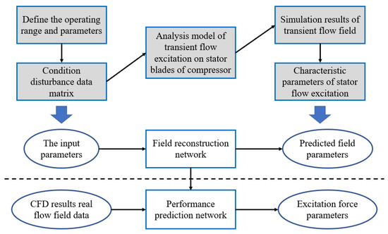
Figure 1.
Overall framework.
Two networks are used to predict the physical field and the excitation characteristics, respectively. The detailed network structure is given later. The flow field reconstruction network was used to establish the compressor stator surface pulsation pressure prediction model. The compressor disturbance condition variable was used as the input parameter, and the transient pulsation pressure distribution of the stator blades was used as the output parameter. The convolutional neural networks were selected to build the analysis model of the compressor stator blade’s condition disturbance excitation. The flow field information of the compressor stator blade is used as the input parameter, and the mean value and amplitude of airflow excitation of stator blade are used as the output parameters to train the convolutional neural network model. Once the well-trained model was obtained, the flow excitation characteristics of stator blades could be predicted by the disturbance variables in any working condition. In the figure, the gray rectangle represents the numerical calculation steps, while the bottom rectangle represents the neural network. In addition, “SCNN architecture” is used later to represent the entire network.
The performance prediction network and the field reconstruction network are the two sub-networks that make up the SCNN framework that has been built in this paper, which is depicted in Figure 1. The design variables are the first network’s input; the second network’s input is flow field information; the latter network’s output is aerodynamic performance targets. The field reconstruction progress can be described as follows:
where the loss function of the field reconstruction network is written as:
where is the design variables, is the predicted flow field, is the true flow field, and is the factors in the network that are to be learned which can be obtained by minimizing when it is subjected to:
where D is the dataset of flow fields obtained by CFD.
Similarly, the performance prediction progress can be expressed as follows:
where the loss function of the performance prediction network is showcased as:
where is the actual aerodynamic performance parameters, is the predicted aerodynamic performance parameters, is the factors in the network that are to be learned which can be obtained by minimizing when it is subjected to:
2.2. Network Structure
The overall framework of the network structure that has been built is detailed in Figure 2, including two sets of network models. One of the network’s functions is the flow field reconstruction. Another function of the network model is the performance prediction.
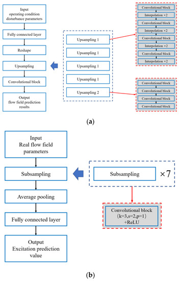
Figure 2.
Network structure. (a) Field reconstruction network; (b) performance prediction network.
For the flow field reconstruction model, the input variables, namely the working condition parameters, are processed by some of the network modules to become the output variables, namely the flow field parameters. In detail, the fully connected layer is used to reconstruct the input variables, which result in a characteristic tensor with two dimensions. Then, in order to match the size of the output variables with the real size of the flow field parameters, some of the operation modules are used to process this part of data so to obtain the real flow field. There are two operations, up-sampling and convolution. For another performance prediction network model, some necessary network operations are applied to convert the real flow field data which are obtained from the CFD results into predicted values of the blade excitation parameters. In detail, a large number of real flow field data which are obtained from CFD numerical simulation are input into the excitation prediction module. Next, in order to obtain the flow excitation parameters of the compressor blades, a series of combined operations are used to transform the flow field data. It includes 7 down-sampling modules. There are also two layers that are used for pooling and full connectivity. It must be explained here that after a successful blade excitation prediction model is constructed through a large amount of data training, the predicted flow field parameters can also be used as its input variables. Using the coupling relationship between the output and output variables, two effective network structures are combined together to form a very complete SCNN network model.
However, in the process of the network’s construction and training, it is easy to encounter two thorny problems, namely slow convergence and gradient explosion. Accordingly, some simple and effective methods have been adopted for data processing to solve these problems. Both the input and output variables in each of the network models were batch normalized. The normalization operation is mainly aimed at performing data preprocessing. For each up-sampling module, it includes four convolution submodules and an activation layer with an ReLU function. In the process of the convolution operation, the convolution kernel size of its module is 3, the operation step size is 1, and the filling size is 1. This paper uses a powerful Adam optimization algorithm to train the structure of the SCNN. For improving the training efficiency, a small batch mode is adopted in the training process. In this paper, 1000 sets of working condition disturbance parameters and part of the corresponding transient pressure pulsation on the stator blade surface are used as the training sample data set.
3. Parametric Methods and Data Collection
3.1. Research Model
The transient flow excitation analysis model of the compressor stator was established. According to the actual equipment that were studied, a three-dimensional flow field CFD model was constructed by the mesh discretion of the rotor and stator blade geometry to verify the solution’s accuracy and the speed of the model, so to meet the steady-state and unsteady solution requirements of high fidelity for the stator blade. Additionally, the 3D flow field model includes a guide moving-vane stator-vane 1.5 level model, which adopts multi-core parallel computing to conduct the CFD simulation of the flow field. In order to reduce the flow channel and save the resources for the transient calculation, the study model was adjusted to include 50 guide blades, 25 rotor blades, and 50 stator blades. The standard operating speed is 3000 rpm. In addition, the subsequent calculation efficiency of working condition disturbance is improved through adaptive numerical model construction, solution, and post-processing, which can meet the needs of large-scale data solutions. Through this model, the simulation analysis and data acquisition of the compressor transient flow excitation are realized efficiently and accurately. Figure 3 shows the numerical model.
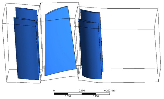
Figure 3.
The numerical model.
3.2. Flow Equations and Meshing
There are three conserved variables in the equation, namely the mass, the momentum, and the energy. For the 3D CFD simulation, it can be uniformly described by the following formula:
In detail, there are three terms in the equation from left to right, which represent the convection term, the diffusion term, and the source term in the flow field. It should be noted that the meaning of φ is a universal variable. If φ is equal to 1, then the equation is continuous. When φ means temperature, the equation becomes an energy equation. Similarly, if φ is the velocity in any direction, the momentum equation is obtained. Γ represents the generalized diffusion coefficient. S represents the source item. the three-dimensional flow of a compressor blade is studied in this paper. The continuum hypothesis and the vortex viscosity hypothesis were adopted. Therefore, the RANS method is used in this paper to simulate the compressor flow field. The Reynolds average method (RANS) is a widely used numerical simulation method of modelling the turbulence in engineering. The turbulence model that was used in this study is k-w. An ideal air condition was used as the working medium. Additionally, the wall surface adopts no slip boundary condition. When the calculated residual is less than 10−5, the calculation is considered to converge.
In order to save the time that it used for data acquisition, the reduced model was used to calculate the compressor blade three-dimensional flow. The mesh generation of the model was performed by calling the TurboGrid macro command in MATLAB. The flow channel is extended axially downstream of the model to enhance the computational convergence. It is helpful to improve the quality of boundary layer meshes by using O-mesh to generate meshes near the blades. For improving the solution accuracy, the mesh density near the front and back edges is increased. Since the mass flow is a working condition parameter in a sample calculation, its calculation accuracy is closely related to the sample data quality. The model that is used in this paper represents the actual equipment in the project, and one working point of the model is used as the reference for grid independence verification in a steady-state calculation. Table 1 shows the research results of grid independence of the model. It can be found that when the grid number increases to 4.4 × 10⁵, the relative deviation of the calculated value of flow is less than 0.4%. So this grid scale is adopted as the benchmark. Figure 4 shows a grid diagram of the fluid domain during the CFD calculation.

Table 1.
Mesh independence study.
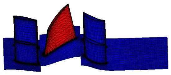
Figure 4.
Mesh of rotor and stationary blades.
3.3. Sample Data Setting
The data matrix of the compressor stator blade in a limited working condition and disturbance range can be generated by self-programming, and the boundary mutation caused by the inlet distortion can be simulated during the operation of the compressor. Thus, the unsteady flow field of a compressor stator blade which is driven by disturbance data is analyzed, and the typical characteristics of the flow excitation on the stator blade surface under the disturbance are obtained. Finally, the corresponding database of the airflow disturbance and stator blade excitation is formed. In the disturbed space, enough sample space should be constructed for the data acquisition to facilitate network learning. Therefore, the quantity and distribution of the data should have sufficient randomness. For the input data, they are distributed using the Latin hypercube sampling method. This method fully guarantees the randomness and uniformity of the samples in the working condition space. Further, within the assumed range of the operating condition disturbance, the sampled samples can cover all of the possible areas without local a concentration phenomenon occurring. In fact, the number of samples is closely related to the accuracy of the model. When the number of samples is too small, the underfitting of the training model leads to a poor prediction accuracy. The selection of the total sample size is positively correlated with the number of input variables and output variables. If the network model has fewer input and output variables, then the required sample size is smaller. When there are more variables, the coupling relationship is very complex, resulting in a very large sample size. In this paper, the LHS method is used to obtain 1000 groups of operating disturbance variables.
For the research model in this paper, if a 20-core CPU was used to solve the problem, then the calculation time for each case would be about half an hour. If the subsequent post-processing and data collation are taken into account, the time of a single case would not exceed 1 h. Two computers were used for the numerical simulation, and the total data preparation time was about 18 days. The disturbance range of the input parameters of the model that is constructed in this study is 8%. So, the data can include a percentage change. Further, if a larger range of percentage data changes is required, the sample extraction of the corresponding range can be carried out in the sampling stage. Of course, this means that the number of samples will increase accordingly. Table 2 shows the parameter ranges. Figure 5 shows the scatter diagram of the relationship between the variables, which shows that there is a high degree of randomness among the variables in the disturbance space.

Table 2.
RANGES OF SAMPLING.
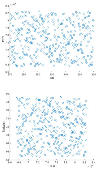
Figure 5.
Data scatter plots.
4. Results and Discussion
4.1. Influence about Training Sizes
Seven groups of data with different training set proportions were selected to train the aforementioned SCNN network model. When the proportion of training set data changes, the prediction error of test set will also change. Figure 6 shows this trend. The flow field is predicted to be the unsteady pressure of a section of blade height on the stator blade surface. The airflow force prediction parameter is the airflow load on the blade, where the FT is the average value of the tangential airflow load, and the FX is the average value of axial load. In addition, “1 order FT” represents the first order tangential airflow force amplitude. Similarly, “1 order FX” represents the force amplitude of the first order axial flow. To further explain the figure below, it is important to point out the definition of the relative error. It represents the average error of all of the predicted values and the real values for the field prediction model. In terms of the load prediction model, the relative error represents the average error between the model prediction parameters of all of the load variables and the real values which are calculated by the CFD.
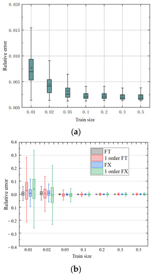
Figure 6.
The trend of model prediction error. (a) Mean prediction error of flow field. (b) Relative error of airflow force prediction.
It can be clearly observed from the figure that the values of the relative error decrease rapidly as the proportion of training sets increases. Additionally, the error tends to be stable when the training set size reaches 0.3. The reason for this phenomenon occurring is that the proportion of data is too low for the small training set, and the constructed neural network system cannot be fully trained. Therefore, the prediction error of lower training set size is large. However, the training effect will not always increase with the increase in the training set size. Because too much training data can easily lead to over fitting of the model. At this time, the network training effect is no longer significantly improved. Therefore, the large training set size prediction error tends to be stable.
For the research in this paper, satisfactory prediction results can be obtained when the training set ratio is 0.3. At this time, the efficiency and accuracy of the neural network model reach a relatively balanced state. Its training effect and resource consumption are considerable. Therefore, only 300 groups of samples are required to participate in the network training for the data that were used in our research. It is very necessary to reduce the consumption of the computing resources in the data preparation stage, which is also conducive to the popularization and application of the model.
4.2. Results of Flow Field Reconstruction
The pressure is the target variable of the flow field reconstruction; the prediction of the pressure is completed at the same time when the model is training. Figure 7 gives the information about the changes with the iteration steps of the loss function in the training process. After several training and testing phases in the network model, the batch size of 32 with a considerable level of accuracy is finally selected. According to the results in the previous section, the training set sample proportion here is defined as 0.3.
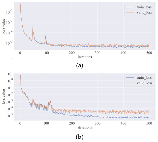
Figure 7.
Change trend of model loss function ((a) Flow field reconstruction model; (b) load prediction model).
It is not difficult to find from the figure that at the beginning, the loss function of both of the network structures decreases very rapidly. While the step of the iteration exceeds 200, the loss function of flow field reconstruction model reaches a small value as the learning rate further decreases. It is 10−5 in the training set, and it is 10−4 in the testing set. Similarly, by observing the training process of the network structure of the incentive prediction, it can be clearly observed that the loss function has the same downward trend. In a word, the training process of network model is complete according to the characteristics of loss function.
Figure 8, Figure 9, Figure 10 and Figure 11 show the real pressure field and the predicted pressure field of 0.1, 0.4, 0.6, and 0.9 stator heights for a specific instance in the test set at different times, respectively. The stationary blade bears the impact of the wake flow of the upper swimming blade, and periodic airflow excitation appears on the blade surface under the unsteady calculation. It can be clearly seen that the surface pressure of different blade height sections undergoes an obvious change at different calculation times. Moreover, the surface trend is basically the same at 0T and T, while the difference is the largest at 0.5T. This corresponds to a complete cycle of airflow excitation.
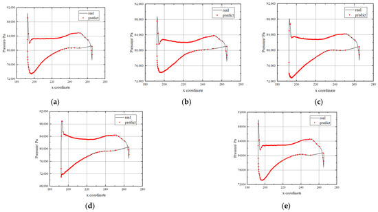
Figure 8.
Unsteady pressure on stator surface at 10% span. (a) t = 0. (b) t = 1/4T. (c) t = 1/2T. (d) t = 3/4T. (e) t = T.
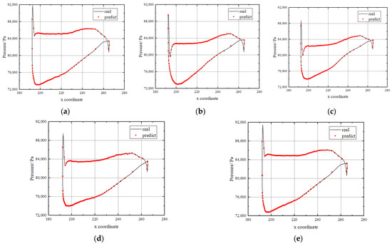
Figure 9.
Unsteady pressure on stator surface at 40% span. (a) t = 0. (b) t = 1/4T. (c) t = 1/2T. (d) t = 3/4T. (e) t = T.
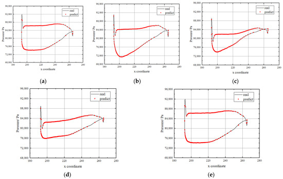
Figure 10.
Unsteady pressure on stator surface at 60% span. (a) t = 0. (b) t = 1/4T. (c) t = 1/2T. (d) t = 3/4T. (e) t = T.
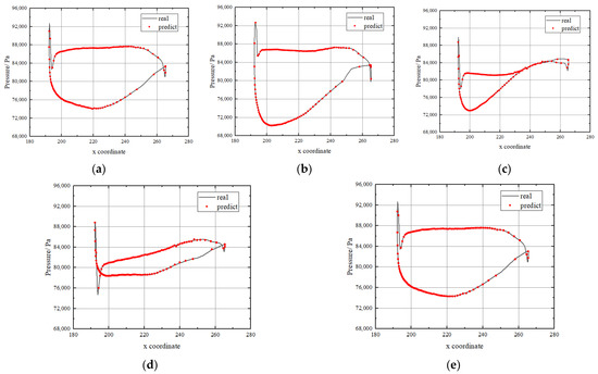
Figure 11.
Unsteady pressure on stator surface at 90% span. (a) t = 0. (b) t = 1/4T. (c) t = 1/2T. (d) t = 3/4T. (e) t = T.
At the same time, it can be seen that the airflow excitation level of the stator at several blade heights is also different, which is reflected in the curve area surrounded by the pressure surface and suction surface. Due to the complex characteristics of the internal flow field of the compressor, the pressure pulsation values at different heights are inconsistent. By comparing all of the pictures, it can be observed that the unsteady prediction data of each section at different times are very close to the numerical curve that was calculated by the CFD. It can be proven that the network performance of flow prediction reaches a high accuracy level. On the other hand, the pressure values at LE and TE of the stator blade changed sharply, which is clearly reflected and accurately predicted in the figure. The results showed that the influence of the wake on the leaves was also clearly reflected. Therefore, the flow field reconstruction network is also very effective in capturing the details of the compressor flow field. In conclusion, this method is very reasonable and reliable for a transient pressure evaluation. Because the two subnetworks are combined, the high prediction accuracy of this network also lays a foundation for the prediction of the airflow excitation.
4.3. Comparison of Performance Prediction
In view of the characteristics of the airflow excitation of the compressor stationary blades, we mainly compared and analyzed the mean and amplitude of the airflow force. The average tangential airflow force data results for all of the validation sets are presented in Figure 12. The excitation prediction model can be used to obtain the average tangential airflow force of the blade under each working condition sample. Additionally, this part of data can be compared and analyzed with the numerical simulation results. The distribution of the predicted values and the actual values as well as the relative error of distribution density can be clearly obtained from the figure.
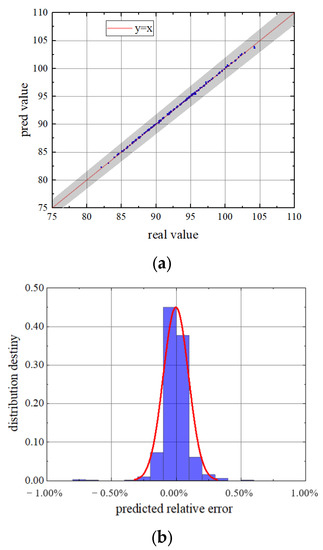
Figure 12.
Mean tangential flow force ((a) Predicted value and true value; (b) relative error density distribution).
It is easy to observe that the prediction error of all of the test sample points is very small. The predicted and actual values of the average tangential load of the blade are in good agreement with y = x ray. All of the points are within the error range of 2%, without there being any exceptions. Additionally, the trend of the distribution density is consistent with the characteristics of the normal distribution. This result reveals the sufficiency of the network training and the accuracy of the model in predicting the average tangential force.
In addition to the mean value of the excitation force, the amplitude of each order of the airflow force load is also an important research parameter for blade vibration. The FFT treatment in this paper ignores the higher-order terms and retains the first-order airflow force amplitude characteristics of the blades under each working condition. For the validation set data, the real value and the predicted value of the first-order amplitude of the tangential airflow force are shown in detail in Figure 13. It is not difficult to find that the tangential airflow force amplitude of the blade has a large variation range due to the disturbance of the operating conditions. This further illustrates the complexity and necessity of studying the blade load under the condition of disturbance. It can be found that the data points of each test set are also very concentrated around y = x. Very few outliers fall outside the 2% error band. Therefore, it is reliable to apply this model to the prediction of airflow excitation with the first-order amplitude of the tangential flow force. Through the above method, the load characteristics of compressor blades can be predicted quickly and accurately.
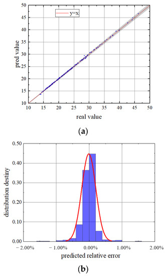
Figure 13.
First order amplitude of tangential flow force ((a) Predicted value and true value; (b) relative error density distribution).
A similar analysis can be performed for the axial flow force of the blade. Here, the model results and the calculated values of the axial force load mean of the compressor stator blade are also shown in Figure 14. It is not difficult to find that the model still achieves a quite satisfactory prediction accuracy. The data points in each validation set fall well within the 2% error band and fit tightly around y = x. In addition, the distribution density of the graph also corresponds to the characteristics of normal distribution. Additionally, it can be found that the mean value of the axial force is smaller than the tangential force is. The same conclusion can be obtained from the results of the first-order axial flow force, as shown in Figure 15. With the exception of a few points that fell outside the 2% margin of error, almost all of the predictions were very accurate. This is because the prediction parameters themselves are small so the error fluctuations that are caused by the disturbance are large. In conclusion, this network model constructed that was In this research could be used to effectively predict the aerodynamic load of the compressor blades.
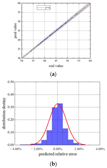
Figure 14.
Mean axial flow force ((a) Predicted value and true value; (b) relative error density distribution).
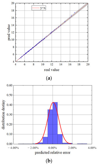
Figure 15.
First order amplitude of axial flow force ((a) Predicted value and true value; (b) relative error density distribution).
In fact, during the numerical analysis in this study, the simulation results of steady-state operating points are consistent with the actual results. Moreover, the data error of airflow force is very small under the design condition. The rationality of the numerical analysis in this paper is verified. The established transient excitation prediction model needs to be further compared with the real operating parameters of the compressor for analysis, and this part of the work needs to be further carried out in the following studies.
5. Conclusions
As far as this study is concerned, the deep learning method is used to carry out the excitation prediction of the compressor stator unsteady flow field. Two network structures are established to connect the compressor operating parameters with the blade flow field parameters and the excitation characteristics. In addition, the aerodynamic characteristics of the compressor under complex working conditions are obtained by an unsteady calculation. A large amount of CFD data were used to train the network model, and good training results have been obtained. Finally, an effective prediction model was formed to analyze the unsteady flow field and the flow force parameters of the compressor stator blades under complex working conditions. The research in this paper contributes a simple and reliable method to the analysis of the compressor blade load under complex working conditions. The main conclusions are as follows:
- (1)
- This paper compares the influence of different training set sizes on the network training effect. In both the flow field prediction model and the blade airflow excitation parameter prediction model, the relative error between the model results and the actual values decreases gradually when the training set size increases gradually. The best training set size is 0.3. In this case, both the flow field and the excitation prediction loss function are reduced to below 10−4. At this time, the relative errors of the model forecasts have been reduced to a considerable level. If the training accuracy is increased, overfitting will occur. It can be seen that the SCNN network model that is presented in this paper can use a small number of CFD data to obtain good training effects and achieve accurate parameter predictions.
- (2)
- A test sample was selected for the study, and the prediction effects for the transient pressure on the stator’s different sections at 0.1, 0.4, 0.6, and 0.9 blade heights were compared and analyzed in detail. It can be found from the results that the flow prediction network has a very good prediction effect on the unsteady pressure. The actual value that was calculated by the CFD is very close to the predicted result of the network model at each time point or blade section. This method can also reliably obtain the flow parameter details of the LE and TE of the stator blade. At the same time, very obvious periodic information of the pressure fluctuations can be obtained by solving an unsteady calculation. It shows that the network that is presented in this paper is accurate and reliable for the prediction of the blade’s transient parameters.
- (3)
- In terms of the compressor flow excitation prediction under complex working conditions, it can be seen that the network model that was trained with 1000 working condition disturbance samples has achieved good results. By comparison, it can be found that the relative errors of both the mean value and the first-order amplitude of the axial and tangential blade airflow loads are very small. Most of the data points were within 2% of the error. Moreover, the predictions of various parameters are in good agreement with the normal distribution. This method of the blade load analysis is efficient and accurate, and it has a good reference value for the blade vibration analysis.
The research of this paper has more scope for further expansion. On the one hand, the airflow load data are combined with the finite element method, and the network model of the blade vibration response and the operating condition disturbance can be analyzed. On the other hand, the excitation characteristics of the compressor rotor blades are more complex, and the method that is proposed in this paper can also be used to predict the load under complex working conditions.
Author Contributions
Each author has contributed different work in this study. J.M. is mainly responsible for data curation, methodology and writing—original draft. The validation and visualization is completed by Z.L., Y.L. undertook the task of supervision and writing—review and editing. Y.X. provides resources. All authors have read and agreed to the published version of the manuscript.
Funding
This research was funded by National Science and Technology Major Project grant number [J2019-IV-0022-0090].
Acknowledgments
All authors in the paper express great gratitude for the financial support by National Science and Technology Major Project (J2019-IV-0022-0090).
Conflicts of Interest
The authors declare that they have no known competing financial interest or personal relationships that could have appeared to influence the work reported in this paper.
References
- Du, Z.; Weng, P.; Zhong, F. Numerical Calculation of Three-dimensional Flow Fields in Turbomachine Blade Rows. J. Eng. Therm. Energy Power 1994, 9, 230–233. [Google Scholar]
- Mailach, R.; Muller, L.; Vogeler, K. Rotor-Stator Interactions in a Four-Stage Low-Speed Axial Compressor—Part II: Unsteady Aerodynamic Forces of Rotor and Stator Blades. J. Turbomach. 2004, 126, 519. [Google Scholar] [CrossRef]
- Cizmas, P.; Dorney, D.J. The Influence of Clocking on Unsteady Forces of Compressor and Compressor Blades. Int. J. Turbo Jet Engines 2000, 17, 133–142. [Google Scholar] [CrossRef]
- Yuan, H.; Yang, W.; Zhao, T.; Liang, M. Effects of stator-rotor interaction on unsteady aerodynamic load of compressor rotor blades. J. Vibroeng. 2015, 17, 2591–2608. [Google Scholar]
- He, L.; Yi, J.; Adami, P.; Capone, L. Space-Time Gradient Method for Unsteady Bladerow Interaction: Part II—Further Validation, Clocking and Multi-Disturbance Effect. J. Turbomach. 2015, 137, 121004.1–121004.12. [Google Scholar] [CrossRef]
- Asghar, M.A.; Liu, Y.; Lu, L. Numerical investigation of unsteady flow interactions in a transonic single stage high pressure compressor. In Proceedings of the 2018 15th International Bhurban Conference on Applied Sciences and Technology (IBCAST), Islamabad, Pakistan, 9–13 January 2018. [Google Scholar]
- Rzadkowski, R.; Gnesin, V.; Kolodyazhnaya, L.; Kubitz, L. Unsteady Forces in Jet Engine 7.5 Compressor Stage. J. Vib. Eng. Technol. 2018, 6, 297–308. [Google Scholar] [CrossRef]
- Voroshnin, D.V.; Marakueva, O.V.; Muraveiko, A.S. Modeling Unsteady Phenomena in an Axial Compressor. Math. Models Comput. Simul. 2020, 12, 413–421. [Google Scholar] [CrossRef]
- Sun, H.; Wang, M.; Wang, Z.; Magagnato, F. Numerical Simulation of the Non-Uniform Flow in a Full-Annulus Multi-Stage Axial Compressor with the Harmonic Balance Method; SAGE PublicationsSage UK: London, UK, 2020. [Google Scholar]
- Williams, D. Review of Current Knowledge on Engine Response to Distorted Inflow Conditions; Defense Technical Information Center: Fort Belvoir, VA, USA, 1987. [Google Scholar]
- Niu, H.; Chen, J.; Xiang, H. Effect of Rotor-Stator Spacing on Compressor Performance at Variable Operating Conditions. Appl. Sci. 2022, 12, 6932. [Google Scholar] [CrossRef]
- Rzadkowski, R.; Soliński, M.; Szczepanik, R. The unsteady low-frequency aerodynamic forces acting on the rotor blade in the first stage of a jet engine axial compressor. In Proceedings of the 10th European Conference on Turbomachinery Fluid Dynamics & Thermodynamics, Lappeenranta, Finland, 15–19 April 2013. [Google Scholar]
- Soliński, M.; Rządkowski, R.; Pająk, A.; Szczepanik, R. The Unsteady Low-Frequency Forces Acting on the Rotor Blade in the First Stage on an Axial Compressor of SO-3 Jet Engine. J. Vib. Eng. Technol. 2014, 2, 385–393. [Google Scholar]
- Yu, C.H.; Li, Q.S.; Yuan, W.; Zhou, S. Boundary condition model for unsteady numerical simulation under inlet distortion. J. Aerosp. Power. 2008, 23, 1695–1700. [Google Scholar]
- Jia, H.X.; Xi, G.; Müller, L.; Mailach, R.; Vogeler, K. Effect of clocking on unsteady rotor blade loading in a low-speed axial compressor at design and off-design operating conditions. Proc. Inst. Mech. Eng. Part G J. Aerosp. Eng. 2008, 222, 895–906. [Google Scholar] [CrossRef]
- Mailach, R.; Vogeler, K. Unsteady Aerodynamic Blade Excitation at the Stability Limit and during Rotating Stall in an Axial Compressor. In ASME Turbo Expo 2006: Power for Land, Sea, and Air vol.6 pt. B: Turbomachinery: Radial Turbomachinery Aerodynamics; Technische Universitaet Dresden Institute for Fluid Mechanics 01062: Dresden, Germany, 2006. [Google Scholar]
- Brunton, S.L.; Noack, B.R.; Koumoutsakos, P. Machine Learning for Fluid Mechanics. Annu. Rev. Fluid Mech. 2020, 52, 477–508. [Google Scholar] [CrossRef]
- Kutz, J.N. Deep learning in fluid dynamics. J. Fluid Mech. 2017, 814, 1–4. [Google Scholar] [CrossRef]
- Zhang, Z.; Song, X.; Ye, S.; Wang, Y.W.; Huang, C.G.; An, Y.R.; Chen, Y.S. Application of deep learning method to Reynolds stress models of channel flow based on reduced-order modeling of DNS data. J. Hydrodyn. 2019, 31, 58–65. [Google Scholar] [CrossRef]
- Wang, Y.; Li, D.; Chen, G. A Reduced-Order Model of Aerodynamic Deep Learning Based on Flow Field Characteristics. In Proceedings of the 4th National Conference on Unsteady Aerodynamics, Hefei, China, 10–13 May 2018. [Google Scholar]
- Han, R.; Wang, Y.; Zhang, Y.; Chen, G. A novel spatial-temporal prediction method for unsteady wake flows based on hybrid deep neural network. Phys. Fluids 2019, 31, 127101. [Google Scholar]
- Hasegawa, K.; Fukami, K.; Murata, T.; Fukagata, K. Machine-learning-based reduced-order modeling for unsteady flows around bluff bodies of various shapes. Theor. Comput. Fluid Dyn. 2020, 34, 367–383. [Google Scholar] [CrossRef]
- Kou, J.; Zhang, W. Multi-fidelity modeling framework for nonlinear unsteady aerodynamics of airfoils. Appl. Math. Model. 2019, 76, 832–855. [Google Scholar] [CrossRef]
- Jiawei, H.U.; Hanru, L.I.U.; Yan’gang, W.; Weixiong, C.H.E.N.; Yan, M.A. Reduced order model for unsteady aerodynamic performance of compressor cascade based on recursive RBF. Chin. J. Aeronaut. 2021, 34, 341–351. [Google Scholar]
- Li, K.; Kou, J.; Zhang, W. Deep neural network for unsteady aerodynamic and aeroelastic modeling across multiple Mach numbers. Nonlinear Dyn. 2019, 96, 2157–2177. [Google Scholar] [CrossRef]
- Du, Q.; Yang, L.; Li, L.; Liu, T.; Zhang, D.; Xie, Y. Aerodynamic design and optimization of blade end wall profile of turbomachinery based on series convolutional neural network. Energy 2022, 244, 122617. [Google Scholar] [CrossRef]
- Du, Q.; Liu, T.; Yang, L.; Li, L.; Zhang, D.; Xie, Y. Airfoil design and surrogate modeling for performance prediction based on deep learning method. Phys. Fluids 2022, 34, 015111. [Google Scholar] [CrossRef]
- Wang, Y.; Liu, T.; Zhang, D. Aerodynamic prediction on the off-design performance of a S-CO2 turbine based on deep learning. In Proceedings of the ASME Turbo Expo 2021, GT2021-60056, Virtual, 7–11 June 2021. [Google Scholar]
- Li, J.; Zhang, M. Data-based approach for wing shape design optimization. Aerosp. Sci. Technol. 2021, 112, 106639. [Google Scholar] [CrossRef]
- Wang, Q.; Zhou, W.; Yang, L.; Huang, K. Comparison between conventional and deep learning-based surrogate models in predicting convective heat transfer performance of U-bend channels. Energy AI 2022, 8, 100140. [Google Scholar] [CrossRef]
Publisher’s Note: MDPI stays neutral with regard to jurisdictional claims in published maps and institutional affiliations. |
© 2022 by the authors. Licensee MDPI, Basel, Switzerland. This article is an open access article distributed under the terms and conditions of the Creative Commons Attribution (CC BY) license (https://creativecommons.org/licenses/by/4.0/).