A Dimension-Reduced Artificial Neural Network Model for the Cell Voltage Consistency Prediction of a Proton Exchange Membrane Fuel Cell Stack

Abstract

The voltage consistency of hundreds of cells in a proton exchange membrane fuel cell stack significantly influences the stack’s performance and lifetime. Using the physics-based model to estimate the cell voltage consistency is highly challenging due to the massive calculation efforts and the complicated fuel cell designs. In this research, an artificial neural network (ANN) model is developed to efficiently predict the cell voltage distribution and the consistency of a commercial-size fuel cell stack. To balance the computation efficiency and accuracy, a dimension-reduced method is proposed with different output-grouping strategies to optimize the ANN structure based on the experiment test of a 100-cell stack. The model’s training time falls nonlinearly from 16 min to 6 s with the output neuron number decreasing from 100 to 5, while the model can still predict the cell voltage distribution trends. With the proposed model, the stack’s cell voltage distributions could be reproduced with significantly lowered computation time, which is beneficial to evaluate the fuel cell status and optimize the control strategies.

1. Introduction

In recent years, there has been an increasing demand for alternative energy due to fossil fuel shortages and environmental issues [1,2,3,4,5,6]. The hydrogen fuel cell technology is an ideal solution, benefiting from low carbon emissions and high energy-conversion efficiency [7,8,9,10,11,12]. As one of the types of fuel cells, the proton exchange membrane fuel cell (PEMFC) has a promising future as a clean power source [13,14,15,16,17,18,19] with its high power density, outstanding energy efficiency, low operating temperature, and zero emissions.

The PEMFC’s commercialization still faces challenges in improving system endurance and performance [20,21], although fundamental research and technology development has been advanced in the past decades. Cell voltage uniformity is one of the significant parameters indicating the performance and endurance of a practical PEMFC stack system [22,23]. Keeping the cell voltage consistent for a stack with hundreds of cells is vital because high cell voltage uniformity ensures a long cell life and high performance [22,24,25]. The cell voltage uniformity is affected by temperature, reactant flow rates, humidity, load current, and gas pressure [24,26,27,28,29].

Two models are used in performance prediction: the physics-based and the data-driven models. The physics-based model demands massive computation resources due to the fact that the designed geometry and multi-physical processes of the fuel cell stack are complicated [24,30]. It makes the model unpractical for performing real-time control and dynamic online diagnostics. Unlike the physics-based model, the data-driven model can reveal the relation between the inputs and the outputs using artificial intelligence algorithms, avoiding the computation of the complex governing equations.

As one of the most widely used data-driven PEMFC models, the artificial neural network (ANN) can process the data efficiently due to the fact that it circumvents the multi-physical mechanism. Several ANN models have been presented for the PEMFC system’s performance forecast and operation optimization. Tian et al. suggested an ANN model coupled with a genetic algorithm to forecast PEMFC performance and determine its maximum power for operational management [31]. Nanadegani et al. developed an ANN model to predict the maximum output power of PEMFCs, taking into account the operational factors’ impact on the polarization curves [32]. Wilberforce and Olabi investigated an ANN model with the group data management approach to forecast fuel cell performance [33]. Asensio et al. devised optimum control techniques to maximize PEMFC efficiency with an ANN model of nonlinear autoregressive configuration. Bhagavatula et al. proposed an ANN structure to forecast the single cell voltage considering the performance impacts of operating circumstances [34]. Han et al. developed an ANN structure and semi-empirical models to find the best working conditions for improving the PEMFC’s efficiency [35]. Yang et al. studied an ANN and multivariate polynomial regression (MPR) model for predicting the short-term degradation behaviors of PEMFCs [36]. Long et al. developed an ANN model to predict the remaining useful life of the PEMFC in comparison with other data-driven models [37]. Wilberforce et al. proposed an ANN model to predict the dynamic electrical and thermal performance of the PEMFC stack under various operating conditions [38,39]. Musharavati et al. investigated a bio-inspired ANN model to find the optimal design and control variables for fuel cell dynamic operations [40].

Most of the literatures focused on the average cell voltage, and did not consider the cell voltage’s uniformity, which is critical to evaluating a fuel cell stack’s performance, health, and reliability. In our previous work [41], an artificial neural network fuel cell model was used to predict each individual cell voltage of a 60 kW PEMFC stack. However, the training and prediction processes are time-consuming for the previous model, of which the computational efficiency should be greatly improved for potential applications in the real-time control and diagnosis of fuel cell engines. In this paper, we propose a dimension-reduced ANN fuel cell model with much less computation effort to study the cell voltage uniformity of a commercial-size 100-cell PEMFC for automotive applications. To reach the best efficiency and accuracy, different structures of the ANN model with various dimension reduction strategies are studied based on the experimental data sets. With the presented model, we reproduce and analyze the uniformity of the cell voltage distributions under various operation and assembly conditions.

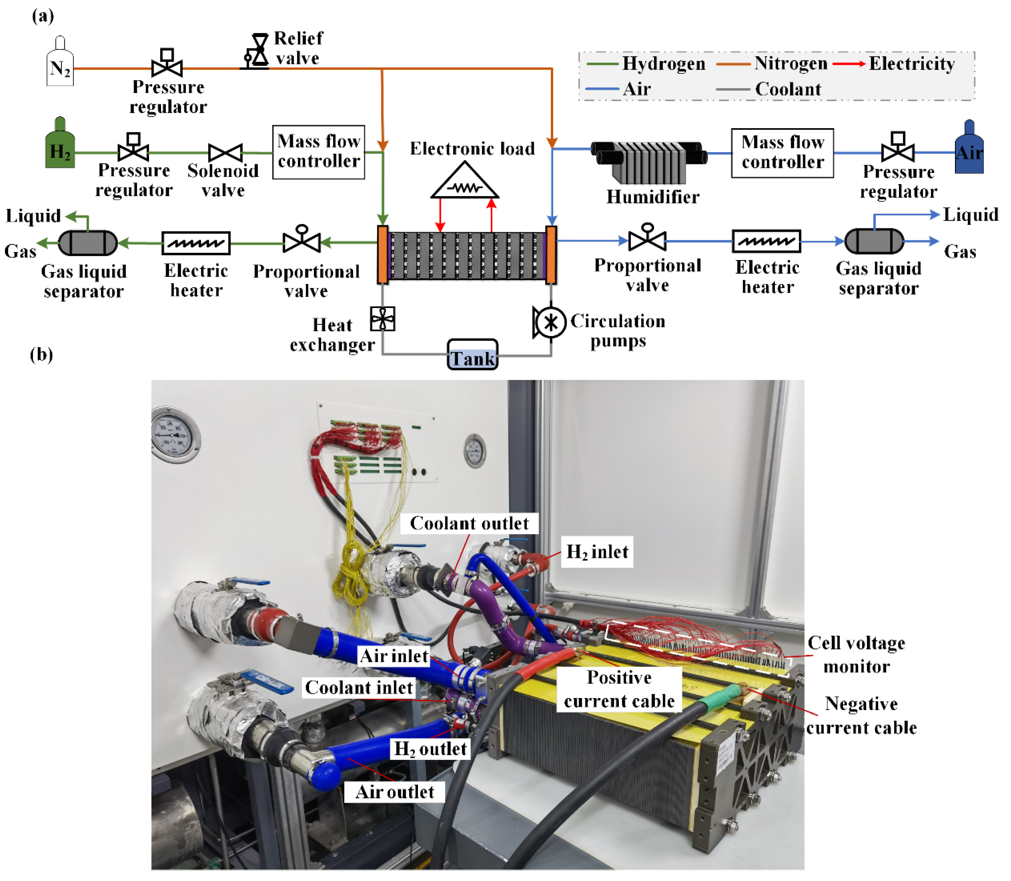
2. Experiment

A lab-built fuel cell testing platform was used to carry out the experimental tests, as shown in Figure 1. The platform contained an air supplier with a humidifier and a mass flow controller (MFC), a hydrogen supplier with a pressure regulator, a solenoid valve and a mass flow controller, a nitrogen supplier with a relief valve and a pressure regulator, a water-cooling system, and a control unit. The hydrogen supplier provided reactant gas to the system, while a respective mass flow controller (MFC) regulated the gas flow rates. The nitrogen supplier worked before and after the experiment to remove the air and the residual reactants inside the pipes and the stack in the device. A water-cooling system controlled the operating temperature and the temperature difference between the inlet and outlet of the stack. In addition, pressure and temperature sensors at the inlet and the outlet of the stack monitored the pressures and the temperatures of the anode, the cathode, and the coolant.

The hydrogen was not humidified in the experiment, while the air was humidified by the wet cathode outlet gas (COG) with a gas-to-gas humidifier to simulate the working condition of the automobile fuel cell system. A constant stoichiometric ratio of $Stoic{h}_A$ = 1.3 for the anode and $Stoic{h}_C$ = 2.0 for the cathode was applied to test the voltage. The stoichiometric ratio is the ratio of the reactant supplied to the required for the electrochemical reaction. With load current densities of less than 0.2 A/cm², which were equal to those at 0.2 A/cm², the constant flow rates were operated for both the anode and the cathode. The cell voltage monitor collected the average voltages in each group of fuel cells in 1 s sampling time, and the recorded results are shown graphically. The operating conditions are listed in

Table 1. Operating conditions.

Parameter	Symbol	Value
Load Current	I	203 A~730.8 A
Stoichiometric Ratio of Hydrogen	λa	1.3
Stoichiometric Ratio of Air	λc	2.0
Assembling Torque	P	12 N.m, 14 N.m, 15 N.m
Coolant Inlet Temperature	Tin	72~75.5 °C
Coolant Outlet Temperature	Tout	74~81 °C

. In the load-changing test, the load current decreased gradually from 730.8 A to 203 A with each change step of 40.6 A. During the test, the stoichiometric ratios of hydrogen and air were kept constant, and the data were sampled at 1 Hz.

3. Model Development

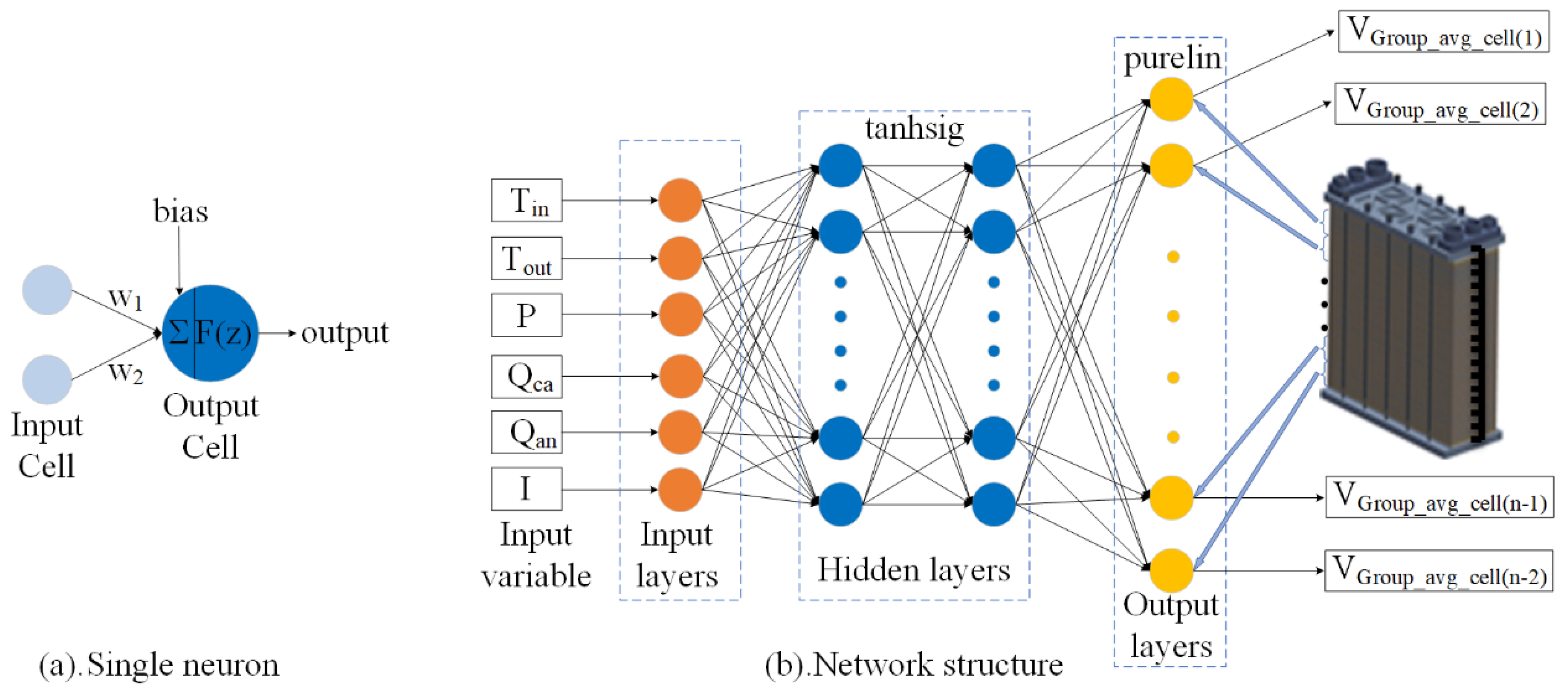
3.1. Artificial Neural Network Model

Inspired by the biological structure of the human brain and neurons, the artificial neural network (ANN) model is one of the most effective and popular tools for data processing. The ANN model, made up of tremendous artificial neurons to imitate how the human brain processes data, is designed to determine the relationship between the input and output values. It is not difficult for a well-trained ANN model to predict the possible output with the input and optimize the functional parameters. In the experiment shown above, a fuel cell ANN model was built to predict the output voltage in a commercial-size PEMFC stack with inputs of operating parameters.

Figure 2a is an example of a single neuron model with multiple inputs and one output, inspired by the synapse. As shown in Figure 2a, a simple neural model has two inputs, one output, and two compute functions. Parameters w1 and w2 are weight values, and bias is the bias value. The first compute function is implemented from a sum function. F(z) is the activation function in the output cell, usually implemented with the Tansig, Purelin, and Sigmoid functions. The Tansig activation function is generally used in hidden layers due to the fact that it is non-linear, and the output value is in the range of [−1, 1]. The Purelin function is used in the output layer because it is a linear function.

The present model had a multi-layer feedforward network architecture containing the input layer, a hidden layer, and the output layer. The input layer consisted of 6 key operating parameters, including the assembling torque (P), coolant inlet temperature ($T_{in}$), coolant outlet temperature ($T_{out}$), flow-rate of hydrogen ($Q_{an}$), flow-rate of air ($Q_{ca}$), and load current (I). Figure 2b shows the proposed ANN model with the six input variables of $T_{in}$, $T_{out}$, $P$, $Q_{ca}$, $Q_{an}$, and I. The model includes two hidden layers with 8 and 5 neurons, respectively. The number of the output-layer neurons is determined by the grouping strategy of the fuel cells, and the output value is the average output voltage in each group of cells. Five ANN models were built to predict the outputs for the different groups of fuel cell performance: 20 cells in 5 groups (D1), 10 cells in 10 groups (D2), 5 cells in 20 groups (D3), 2 cells in 50 groups (D4), and 1 cell in 100 groups (D5). In the following sections, the models with different group designs are compared to study the model’s computation efficiency and prediction precision with varied output complexities.

During the training process, the Levenberg–Marquardt algorithm was used to train the feed-forward network model. One of the advantages of the Levenberg–Marquardt algorithm is that it could not only solve non-linear problems but also optimize parameters using the Gauss–Newton algorithm and the gradient descent method. The outputs were generated from the proposed ANN model based on the given input and target data sets. They had an implicit relationship with input parameters, which could be generalized with the following function:

$$j=F(I,Q_{an},Q_{ca},T_{in},T_{out},P)$$

(1)

3.2. Training Procedure

Forward transmission and backpropagation were the two main methods in the neural network training process. To obtain an efficient calculation, we applied the min-max normalization to adjust the input data before the forward transmission process started. We also used the MATLAB build-in function, “The Mapminmax”, during the training process. It first maps the input data matrix in each row into the range of [−1, 1]. Then, the minimum and the maximum values in those matrix rows were set to either −1 or 1.

$$y=(y_{\max }-y_{\min })\cdot (x-x_{\min })/(x_{\max }-x_{\min })+y_{\min }$$

(2)

In the function above, $y_{\max }$ and $y_{\min }$ are the anticipative minimum and maximum values in each row, x is the input data in this row, and $x_{\max }$ and $x_{\min }$ are the minimum and the maximum in the original input values in the row.

For the $j_{{}^{th}}$ neuron at the $l_{{}^{th}}$ layer, the output $a_j^l$ is expressed in the following mathematical formula:

$$a_j^l=\delta ({\displaystyle \sum _k{w}_{jk}^l{a}_k^{l-1}+b_j^l})$$

(3)

In the function above, $w_{jk}^l$ is the parameter indicating the weight of the relation between neuron k at layer l − 1 and neuron j at layer l, $b_j^l$ is the bias value for neuron j at layer l, and $\delta$ is the activation function used in the hidden layer (tansig) and the output layer (Purelin), which is shown as follows:

$$F(z)=\frac{1-e^{-x}}{1+e^{-x}}$$

(4)

$$F(z)=z$$

(5)

The following matrix shows the process of forward transfer:

$$a^l=\delta (w^l{a}^{l-1}+b^l)$$

(6)

In matrix (6), $w^l$ is the weight matrix (7), $b^l$ is the bias matrix (8), $a^l$ is the output matrix (9) of the l layer, and $a^{l-1}$ is the output matrix (10) of the upper-level layer.

$$w^l=\left[\begin{array}{cccc}{w}_{11}^l& w_{12}^l& \cdots & w_{1n}^l\\ w_{21}^l& w_{22}^l& \cdots & w_{1n}^l\\ ⋮& ⋮& \ddots & ⋮\\ w_{n1}^l& w_{n1}^l& \cdots & w_{nn}^l\end{array}\right]$$

(7)

$$b^l=\left[\begin{array}{c}{b}_1^l\\ b_2^l\\ ⋮\\ b_n^l\end{array}\right]$$

(8)

$$a^l=\left[\begin{array}{c}{a}_1^l\\ a_2^l\\ ⋮\\ a_n^l\end{array}\right]$$

(9)

$$a^{l-1}=\left[\begin{array}{c}{a}_1^{l-1}\\ a_2^{l-1}\\ ⋮\\ a_n^{l-1}\end{array}\right]$$

(10)

The cost function was introduced to characterize and optimize the prediction precision of the ANN model. During the training process of artificial neural networks, it is necessary to find the optimized parameters (weights and offsets) minimizing the value of cost function, which indicates the deviation between the predicted and tested values. To minimize the cost function’s (11) value, the derivatives of the internal parameters (gradient to be exacted) of the ANN model are calculated and updated step by step according to the gradient-decent method by a backpropagation algorithm. For gradient-decent optimization, the parameters are calculated using the Levenberg–Marquardt algorithm, which combines the characteristics of the Newton method and the gradient method to compute more efficiently.

$$C=-\frac{1}{m}{\displaystyle \sum _{i=0}^m(y^i\cdot \log (a^i)+(1-y)\cdot \log (1-a^i))}$$

(11)

To improve the prediction accuracy, the mean square error (MSE) and the coefficient of determination (R²) are calculated using the Formulas (12) and (13), respectively.

$$MSE=\frac{1}{N}{\displaystyle \sum _{t=1}^N{(V_{ANN,cell}-V_{test,cell})}^2}\times 100\%$$

(12)

$$R^2=1-{\displaystyle \sum _{t=1}^N{(V_{ANN,cell}-V_{test,cell})}^2}/{\displaystyle \sum _{t=1}^N{(V_{ANN,cell}-{\overline{V}}_{test,cell})}^2}$$

(13)

where N indicates the number of data samples, $V_{ANN,cell}$ is the predicted cell voltage, $V_{test,cell}$ is the tested cell voltage, and ${\overline{V}}_{test,cell}$ is the average voltage.

The ANN models presented in this paper were built with MATLAB’s neural network tools, such as dynamic networks, radial basis kernel functions, and feed-forward algorithms. The build-in network function was also used in the modeling process to generate a custom neural network. To optimize the network, the parameters such as validation checks, gradient, MSE, and epoch were adjusted to reach the best output result. Each parameter had a significant effect on the outcome of the model. For example, the parameter epoch meant that every sample in the training set was learned by the model once for each epoch. Thus, the epoch determined the iterative learning times for the forward and back propagation during the model training process. The vector gradient indicated the largest directional derivative in its direction; the validation checks were the iteration times for computing termination, of which the model calculation error for each iteration remained stable. In the training process, the epoch was set to be 1000 times, the gradient was $1\times {10}^{-5}$, and the validation checks number was 6. The training would end if one of these results met these conditions.

4. Results and Discussion

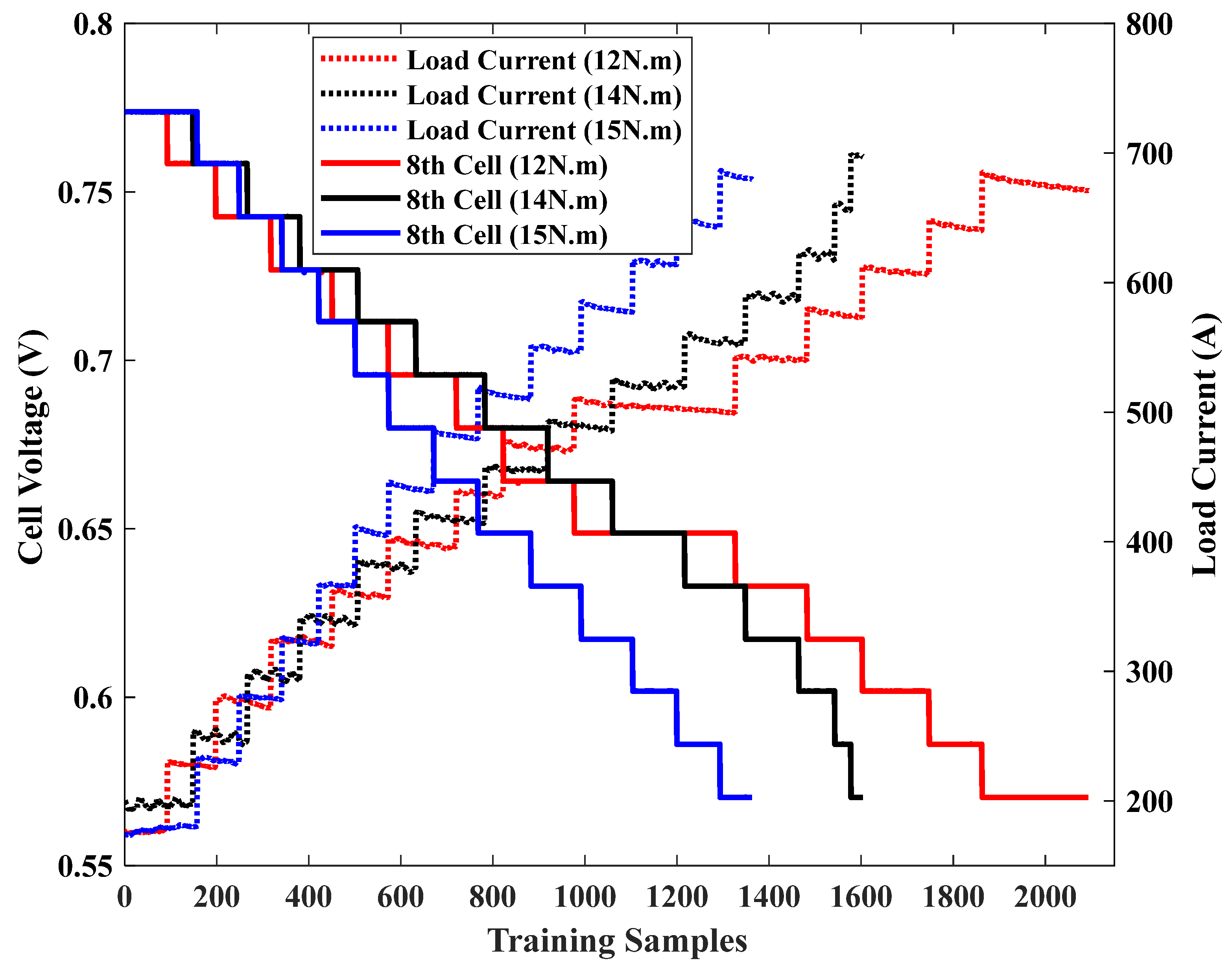
4.1. Experimental Results and Training Data Preprocessing

As Figure 3a shows, the 12 N.m assembly torque group has the best performance over the entire load current range, indicating the optimized assembly torque of the presented fuel cell stack. At load currents lower than 550 A, the 14 N.m assembly torque group performs similarly to the 15 N.m assembly torque group. However, the voltages of the 14 N.m group show the lowest values while the load current is higher than 550 A. This deviation keeps increasing with the ascending load current.

From the results presented in Figure 3b, we can conclude that the air pressure difference grows larger if the assembly torque is higher. This difference is also affected by the load current: the difference is bordered while the load current is increased. The gas consumption increases as the load current grows under the given reactants’ stoichiometric ratios.

The cell voltage varies under different assembling torques of 12 N.m, 14 N.m, and 15 N.m, with the load current increasing at the step of a constant 0.1 A/cm². The performance in the eighth cell is shown in Figure 4. The load current decreases from 1.8 A/cm² to 0.5 A/cm² while the cell voltage increases from ~0.56 V to ~0.78 V under the assembling torques of 12 N.m and 14 N.m and from ~0.6 V to ~0.81 V at 15 N.m. For the training samples, the cell voltage experiment data of the dynamic overshooting process during the load current descending are removed because the data deviate significantly from the steady-state results.

The experiment results are divided into three data sets: 70% are the data-for-training set, 15% are the validation set, and 15% are the test set. The training set is used to train the network model, the validation set is used to validate the network parameters, and the test set is used to test the prediction performance of the model. The model performance is considered based on the parameters of R², MSE, and training time, as shown in

Table 2. MSE, R², Training Time, and the ANN structure in each group.

	ANN Structure	R2	MSE	Training Time
D1	6-8-5-5	0.99992	5.2523 × 10−7	6 s
D2	6-8-5-10	0.99992	5.9548 × 10−7	23 s
D3	6-8-5-20	0.99992	6.8463 × 10−7	17 s
D4	6-8-5-50	0.99991	6.3335 × 10−7	302 s
D5	6-8-5-100	0.99990	7.6788 × 10−7	977 s

. The computer, for the model computation using the MATLAB neural network toolbox, has the specifications of an Intel^® Core™ [email protected] processor and a single-channel 8GB@2133MHz memory.

4.2. ANN Structure and Model Validation

The predicted results for each group of fuel cells are shown in Figure 5, and the grouping strategy is shown in Table 2. The number of cells in each group decreases from D1 (6-8-5-5) to D5 (6-8-5-100): D1 (6-8-5-5) has five groups of data that have an average voltage of twenty cells; D2 (6-8-5-10) has ten groups of data and ten cells in each group; D3 (6-8-5-20) has twenty groups of data with the average voltage of five cells; D4 (6-8-5-50) has fifty groups of data with two cells in each; D5 (6-8-5-100) has a hundred groups of data with one cell in each group. Due to the fact that there are more groups in D5 (6-8-5-100), the corresponding regression line has more data points and seems thicker. All of these predictions pass the test with high accuracies of $R^2\ge 0.9999$.

Meanwhile, more data groups require a longer time to train the ANN model with relatively higher MSEs. The training D5 (6-8-5-100) consumes much more time than D4 (6-8-5-50). It is found that the time needed grows exponentially. Compared with building a model such as D5 (6-8-5-100), a model such as D4 (6-8-5-50) requires a much shorter time and lower MSE. This is because the model could not predict well under a smaller current, and the more data points the model has, the lower its accuracy would be.

Admittedly, the gap in training time would be narrowed if the hardware configuration was upgraded, and the result could have higher accuracy with more data groups. However, a good grouping strategy contributes to a higher processing efficiency, especially when a considerable amount of experiment data needs to be processed online.

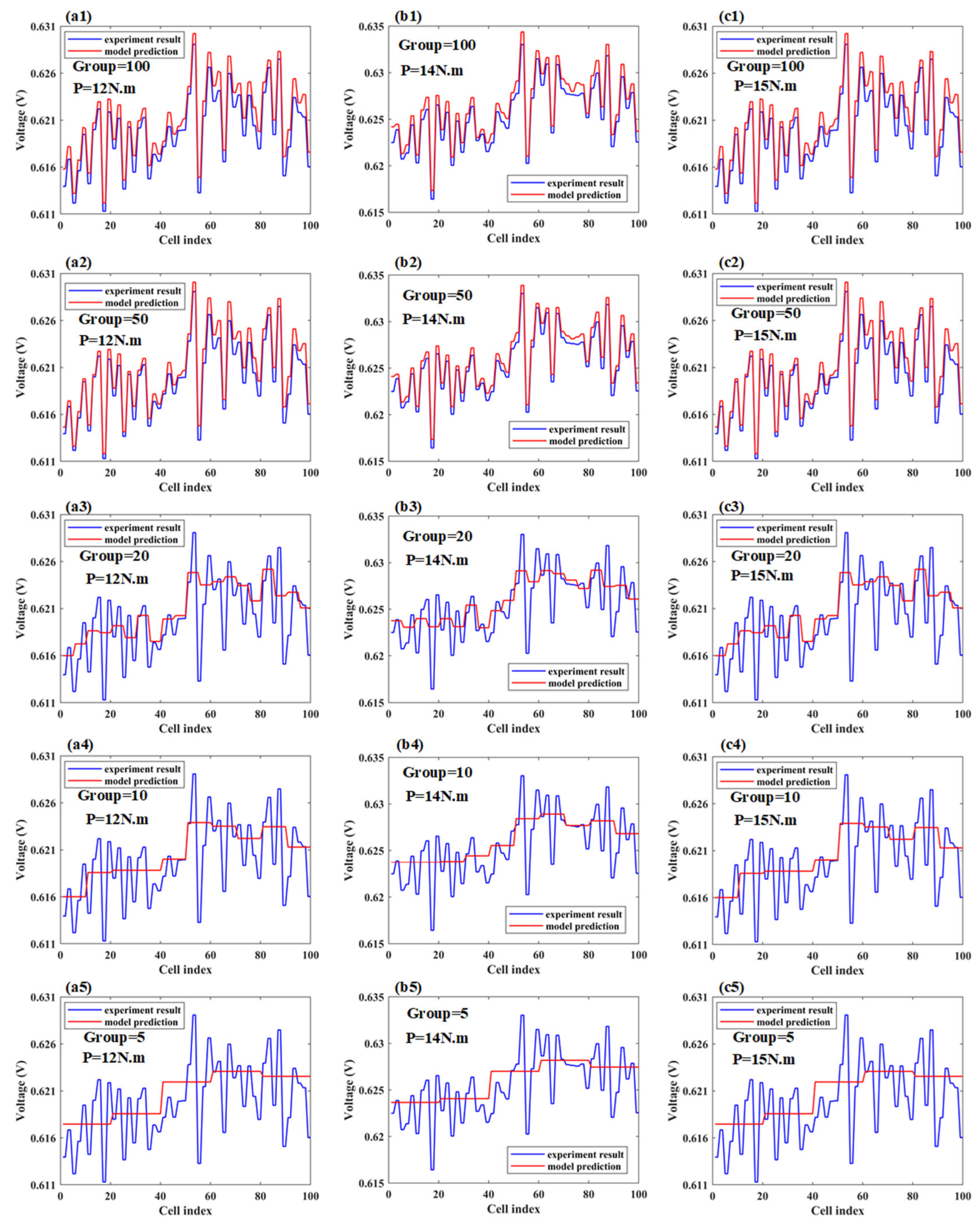
4.3. Performance Prediction and Analysis

The cell voltage uniformity ($U_{cell}$) (14) and range (15) are parameters used for evaluating the stack voltage consistency. The cell voltage uniformity shows the dispersion of the voltages in cells, and it can be expressed as the following:

$$U_{cell}=\sqrt{\frac{1}{N}{\displaystyle \sum _{i=1}^N{(V_i-\overline{V})}^2}}$$

(14)

The range is the difference between the maximum and minimum cell voltages, illustrating the magnitude of the fluctuation in cell voltages. The range is calculated as the following:

$$Range=V_{max}-V_{\min }$$

(15)

The tested voltage distributions and model predicted outputs of 100 cells with the same current density but different assembly torques are shown in Figure 6. All of the subgraphs have a longitudinal span of 0.02 V. The more significant the fluctuation within the same variation range of the longitudinal axis, the worse the cell’s consistency. Figure 6(a2,b2,c2) compares the model’s predicted outputs to the tested results of the 50 groups with two cells.

Under different assembly torques, all of the model predictions match the experimental results closely, and the predicted outputs are always higher than the tested. The model predicts accurately when the assembly torque is 14 N.m. When the assembly torques are 12 N.m or 15 N.m, a voltage deviation about 2 mV is observed around the 95th cell between the model and experiment results. When the assembly torque is 12 N.m, the graph has the lowest fluctuation amplitude, indicating that this is the best cell voltage consistency of the fuel cell stack. The comparisons of predicted and tested outputs in the 100 and 50 groups are shown in Figure 6(a1,a2,b1,b2,c1,c2). The model’s predictions of the cell voltage distributions fit well with those of the experimental results and provide detailed information of individual cell voltages. Figure 6(a3,b3,c3) presents a comparison of the predicted outputs and experimental results of the 20 groups of cells each with 5 cells. As the number of the group (output dimension) is reduced, the predicted results lose detailed cell voltage information but retain the distribution trends of the stack for potential status evaluation of the fuel cell. The comparisons within Figure 6(a4,a5,b4,b5,c4,c5) show that more details of cell voltage distribution are lost as the number of groups decreases. The diagram should be a straight line parallel to the x-axis when there is only one group, showing only the average voltage of the 100 cells and missing the cell voltage distribution information.

Figure 7 shows the cell voltages of model predictions and experiment findings with a constant assembly torque of 14 N.m but with varied grouping strategies and load currents. Under varying assembly torques, all predictions match the experimental results closely, and the predicted outputs are generally slightly greater than the tested ones. The cell voltage consistency decreases across all groups as the load current increases, and the fluctuation becomes more pronounced in the groups with more data groups. Furthermore, as the load current grows, the prediction accuracy improves. The detail losses in D3 (6-8-5-20), D2 (6-8-5-10), and D1 (6-8-5-5) described in Figure 6 persist. For example, the prediction results of Figure 7(c4,c5) fail to reflect the detailed voltage fluctuations of the local cell voltage around the 75th cell, while the prediction curves of Figure 7(c1,c2,c3) could follow the experimental results with detailed voltage distributions. This is mainly attributed to the dimension-reduction of the voltage output for the model. When the number of data groups diminishes, the data input becomes insufficient for artificial intelligence to anticipate the curve in detail. Furthermore, the peak, as mentioned earlier, and valley of the curves are not shown in these groups, while the curve in these groups clearly illustrates the trend in cell voltages.

In Figure 8, groups D4 (6-8-5-50) and D5 (6-8-5-100) reach the curves close to the experimental result of the $U_{cell}$ and the range. However, for groups D1 (6-8-5-5), D2 (6-8-5-10), and D3 (6-8-5-20), there is a gap between the predicted and the experimental curves, and the gap is broader in the groups with fewer data groups. The gap keeps increasing as the load current increases. In Figure 8(b1), all of the predicted and experimental results have lower starting and ending $U_{cell}$, indicating better cell voltage uniformity. Similarly, the starting and ending ranges of all groups in Figure 8(b2) are also lower than those in Figure 8(a2,c2), as is consistent with the result of $U_{cell}$. At the starting point, the $U_{cell}$ difference in all groups is relatively small, but the gap is increasingly broadened at the points where a 330 A load current is applied. Unlike the $U_{cell}$ difference, the range difference in different groups also increases as the load current increase, but it is evident at a low load current. Under a high load current, the predicted range curves in the D1 (6-8-5-5), D2 (6-8-5-10), and D3 (6-8-5-20) groups show diversion both in the increasing gap between the $U_{cell}$ predictions of larger group numbers and smaller group numbers at 330 A and in the significantly increasing gap between D3 (6-8-5-20), D2 (6-8-5-10), and D1 (6-8-5-5) at a load current around 650 A.

In contrast, the $U_{cell}$ curve does not show this diversion. Figure 8(b1,b2) shows that D5 (6-8-5-100) and D4 (6-8-5-50) do not fit the experimental results well at a low load current under assembly torque 14 N.m, but that the gap is eliminated at around 330 A. Additionally, the fluctuation of Figure 8(b1,b2) for groups D3 (6-8-5-20), D2 (6-8-5-10), and D1 (6-8-5-5) is higher than the curves of the same groups in Figure 8(a1,a2) or Figure 8(c1,c2).

Figure 8 (a1,b1c1) shows the predicted and tested $U_{cell}$ under changing currents with different assembly torques and grouping strategies. In the D4 (6-8-5-50) and D5 (6-8-5-100) groups, the predicted outputs match the experimental results closely, but in D3 (6-8-5-20), D2 (6-8-5-10), or D1 (6-8-5-5) the predicted $U_{cell}$ decreases as the number of the group decreases due to the detail losses in cell voltage distribution as the number of group decreases. Interestingly, D3 (6-8-5-20) has a higher predicted $U_{cell}$ than that of D4 (6-8-5-50) at the assembly torque of 14 N.m and at the load currents from 500 A to 600 A. This is possibly due to the overall consistency of every five neighboring cells being better than every ten neighboring cells within this load current range. The three figures above also show that when the assembly torque is 14 N.m, the predicted and tested results have the lowest $U_{cell}$ under different groups. For example, when the current load is 732 A and the assembly torque is 14 N.m, the experimental and predicted results are lower than 5.5 mV. In contrast, when the assembly torque is 12 N.m or 15 N.m, the experimental and the predicted results are around 6.5 mV. However, the assembly torque of 15 N.m is more consistent than that of 12 N.m at low-current loads. The maximum predicted and tested values at 15 N.m are approximately 1.5 mV, whereas the maximum values are approximately 2 mV when the current load is 12 N.m.

We conclude that the cell’s consistency deteriorates as the current load increases based on the three figures above. In D5 (6-8-5-100) and D4 (6-8-5-50), the increase in consistency is exponential, while the consistency changes are essentially linear for D3 (6-8-5-20), D2 (6-8-5-10), and D1 (6-8-5-5), with the slope decreasing as the number of groups decreases. In the case of a high-load current and an assembly torque at 12 N.m, D4 (6-8-5-50) and D5 (6-8-5-100) even show a logarithmic growth trend. This is because under high-current loads, the rapid flow rate of reaction gas in the reactor has distributed flow field that can result in a turbulent and unstable gas supply. The reaction flow rate and consumption are moderate in the middle range of the load current, and the fluid distribution of each cell is stable, leading the uniform distribution of cell voltages.

Figure 8 (a2,b2,c2) depicts the predicted and tested ranges with different load currents, assembly torques, and grouping strategies. The range has a similar growing trend to the $U_{cell}$, but the fluctuations in range are smaller. The predicted and tested ranges in each group under different load currents are the smallest when the assembly torque is 14 N.m. When the assembly torque is 12 N.m or 15 N.m, the maximum predicted and tested values are around 28 mV, while they are 25 mV at 14 N.m. In D4 (6-8-5-50) and D5 (6-8-5-100), both the predicted and tested range curves show an exponential growth trend with increasing current load; in D3 (6-8-5-20), D2 (6-8-5-10), and D1 (6-8-5-5), the linear growth trend is shown, but the slope is lower, and the change is gentler compared with the curve of the $U_{cell}$. High ranges may trigger cell voltage drops, resulting in irreversible fuel cell degradation. As a result, a high range should be avoided even if the $U_{cell}$ values are low.

5. Conclusions

In this study, a dimension-reduced ANN model is proposed to predict the cell voltage distributions of a 100-cell automobile PEMFC stack. The cell voltage consistency is analyzed with varied ANN model structures under different fuel cell operating and assembly conditions. The primary findings are as follows:

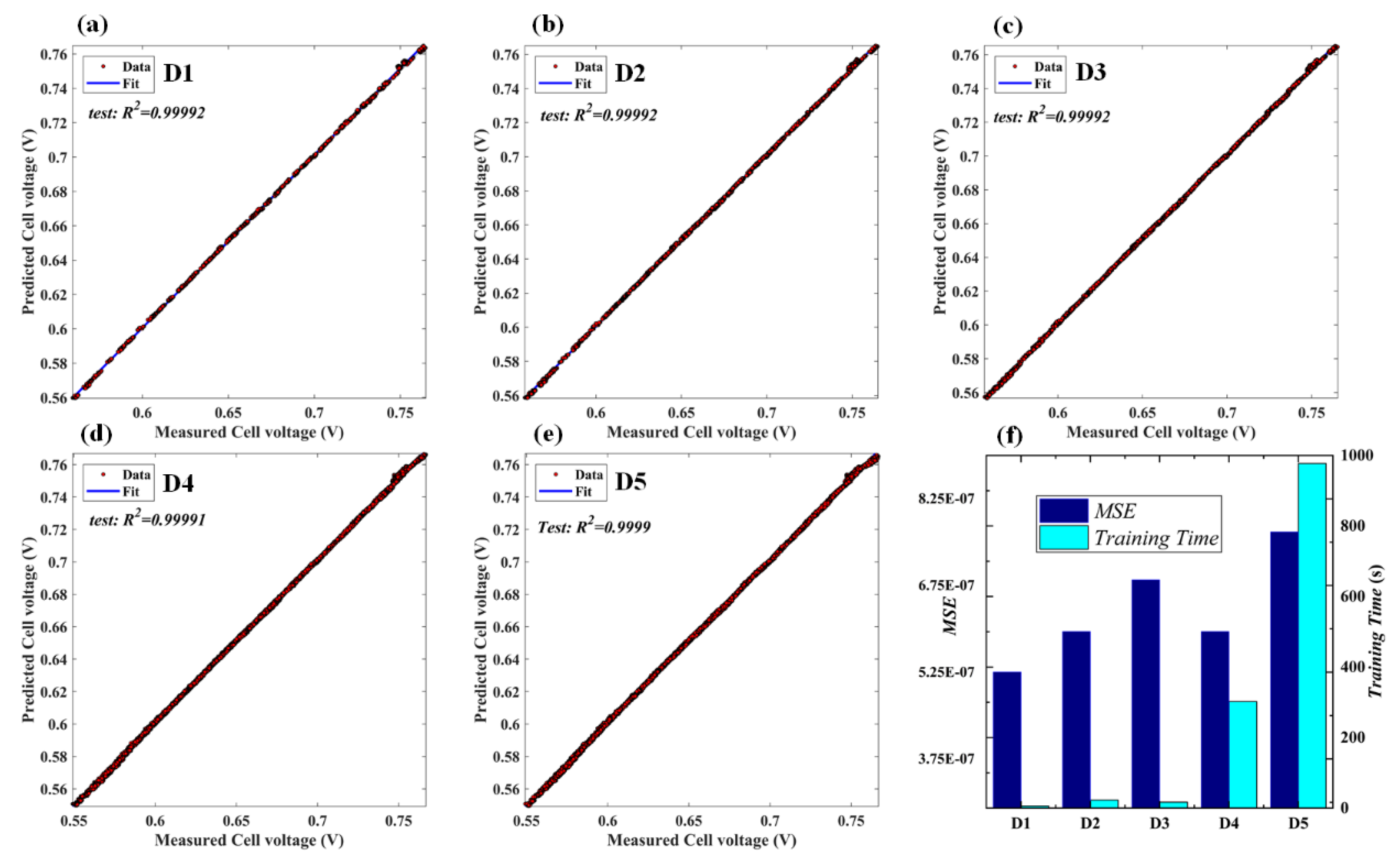
• Five grouping strategies for the output values are applied for the ANN model. All of the model structures have a good prediction accuracy, with R² values greater than 0.999. The predictions under different stack assembly torques fit the experimental results, with margins of error less than 2 mV.
• The ANN model can accurately predict each group’s average voltage under different group strategies. The MSE values of the proposed models are lower than 8 × 10⁻⁷. With the reduced output dimension of the model, details of the individual cell voltages are missed, but the distribution trends of the cell voltage distributions are retained.
• The training time decreases as the number of cells in each group decreases. The minimum training time for the five data groups is only six seconds.
• The $U_{cell}$ and range values positively correlate with the load currents under different assembly torques, while the curve slope declines as the model output dimension reduces.

References

- Qiu, D.; Peng, L.; Shen, S.; Lai, X. Analysis of degradation mechanism in unitized regenerative fuel cell under the cyclic operation. Energy Convers. Manag. 2022, 254, 115210. [Google Scholar]
- Yin, C.; Gao, Y.; Li, K.; Wu, D.; Song, Y.; Tang, H. Design and numerical analysis of air-cooled proton exchange membrane fuel cell stack for performance optimization. Energy Convers. Manag. 2021, 245, 114604. [Google Scholar] [CrossRef]
- Wan, Y.; Qiu, D.; Yi, P.; Peng, L.; Lai, X. Design and optimization of gradient wettability pore structure of adaptive PEM fuel cell cathode catalyst layer. Appl. Energy 2022, 312, 118723. [Google Scholar] [CrossRef]
- Zhao, J.; Cai, S.; Luo, X.; Tu, Z. Dynamic characteristics and economic analysis of PEMFC-based CCHP systems with different dehumidification solutions. Int. J. Hydrogen Energy 2022, 47, 11644–11657. [Google Scholar] [CrossRef]
- Yin, C.; Gao, Y.; Li, K.; Song, Y.; Tang, H. Experimental Investigation on Local Behaviors of PEMFC with Segmented Cell. Automot. Innov. 2021, 4, 165–175. [Google Scholar] [CrossRef]
- Bai, X.; Luo, L.; Huang, B.; Huang, Z.; Jian, Q. Flow characteristics analysis for multi-path hydrogen supply within proton exchange membrane fuel cell stack. Appl. Energy 2021, 301, 117468. [Google Scholar] [CrossRef]
- Huang, W.; Jian, Q.; Feng, S.; Huang, Z. A hybrid optimization strategy of electrical efficiency about cooling PEMFC combined with ultra-thin vapor chambers. Energy Convers. Manag. 2022, 254, 115301. [Google Scholar] [CrossRef]
- Bai, X.; Jian, Q.; Huang, B.; Luo, L.; Chen, Y. Hydrogen starvation mitigation strategies during the start-up of proton exchange membrane fuel cell stack. J. Power Sources 2022, 520, 230809. [Google Scholar] [CrossRef]
- Yin, C.; Gao, J.; Wen, X.; Xie, G.; Yang, C.; Fang, H.; Tang, H. In situ investigation of proton exchange membrane fuel cell performance with novel segmented cell design and a two-phase flow model. Energy 2016, 113, 1071–1089. [Google Scholar] [CrossRef]
- Zhao, J.; Tu, Z.; Chan, S.H. In-situ measurement of humidity distribution and its effect on the performance of a proton exchange membrane fuel cell. Energy 2022, 239, 122270. [Google Scholar] [CrossRef]
- Yin, C.; Song, Y.; Liu, M.; Gao, Y.; Li, K.; Qiao, Z.; Tang, H. Investigation of proton exchange membrane fuel cell stack with inversely phased wavy flow field design. Appl. Energy 2022, 305, 117893. [Google Scholar] [CrossRef]
- Gong, C.; Du, Y.; Yu, Y.; Chang, H.; Luo, X.; Tu, Z. Numerical and experimental investigation of enhanced heat transfer radiator through air deflection used in fuel cell vehicles. Int. J. Heat Mass Transf. 2022, 183, 122205. [Google Scholar] [CrossRef]
- Huang, F.; Qiu, D.; Peng, L.; Lai, X. Optimization of entrance geometry and analysis of fluid distribution in manifold for high-power proton exchange membrane fuel cell stacks. Int. J. Hydrogen Energy 2022, 47, 22180–22191. [Google Scholar] [CrossRef]
- Bai, X.; Luo, L.; Huang, B.; Jian, Q.; Cheng, Z. Performance improvement of proton exchange membrane fuel cell stack by dual-path hydrogen supply. Energy 2022, 246, 123297. [Google Scholar] [CrossRef]
- Yang, L.; Cao, C.; Gan, Q.; Pei, H.; Zhang, Q.; Li, P. Revealing failure modes and effect of catalyst layer properties for PEM fuel cell cold start using an agglomerate model. Appl. Energy 2022, 312, 118792. [Google Scholar] [CrossRef]
- Wu, D.; Peng, C.; Yin, C.; Tang, H. Review of System Integration and Control of Proton Exchange Membrane Fuel Cells. Electrochem. Energy Rev. 2020, 3, 466–505. [Google Scholar] [CrossRef]
- Yin, C.; Gao, Y.; Li, T.; Xie, G.; Li, K.; Tang, H. Study of internal multi-parameter distributions of proton exchange membrane fuel cell with segmented cell device and coupled three-dimensional model. Renew. Energy 2020, 147, 650–662. [Google Scholar] [CrossRef]
- Yin, C.; Cao, J.; Tang, Q.; Su, Y.; Wang, R.; Li, K.; Tang, H. Study of internal performance of commercial-size fuel cell stack with 3D multi-physical model and high resolution current mapping. Appl. Energy 2022, 323, 119567. [Google Scholar] [CrossRef]
- Chen, X.; Yang, C.; Sun, Y.; Liu, Q.; Wan, Z.; Kong, X.; Tu, Z.; Wang, X. Water management and structure optimization study of nickel metal foam as flow distributors in proton exchange membrane fuel cell. Appl. Energy 2022, 309, 118448. [Google Scholar] [CrossRef]
- Ahn, S.Y.; Shin, S.J.; Ha, H.Y.; Hong, S.A.; Lee, Y.C.; Lim, T.W.; Oh, I.H. Performance and lifetime analysis of the kW-class PEMFC stack. J. Power Sources 2002, 106, 295–303. [Google Scholar] [CrossRef]
- Barzegari, M.M.; Rahgoshay, S.M.; Mohammadpour, L.; Toghraie, D. Performance prediction and analysis of a dead-end PEMFC stack using data-driven dynamic model. Energy 2019, 188, 116049. [Google Scholar] [CrossRef]
- Dai, C.; Shi, Q.; Chen, W.; Li, Y.; Li, Q. A review of the single cell voltage uniformity in proton exchange membrane fuel cells. Proc. CSEE 2016, 36, 1289–1302. [Google Scholar]
- Zhu, W.H.; Payne, R.U.; Cahela, D.R.; Tatarchuk, B.J. Uniformity analysis at MEA and stack Levels for a Nexa PEM fuel cell system. J. Power Sources 2004, 128, 231–238. [Google Scholar] [CrossRef]
- Futter, G.A.; Latz, A.; Jahnke, T. Physical modeling of chemical membrane degradation in polymer electrolyte membrane fuel cells: Influence of pressure, relative humidity and cell voltage. J. Power Sources 2019, 410, 78–90. [Google Scholar] [CrossRef]
- Chen, K.; Hou, Y.; Jiang, C.; Pan, X.; Hao, D. Experimental investigation on statistical characteristics of cell voltage distribution for a PEMFC stack under dynamic driving cycle. Int. J. Hydrogen Energy 2021, 46, 38469–38481. [Google Scholar] [CrossRef]
- Asensio, F.J.; Martin, J.I.S.; Zamora, I.; Onederra, O. Model for optimal management of the cooling system of a fuel cell-based combined heat and power system for developing optimization control strategies. Appl. Energy 2018, 211, 413–430. [Google Scholar] [CrossRef]
- Laribi, S.; Mammar, K.; Sahli, Y.; Koussa, K. Air supply temperature impact on the PEMFC impedance. J. Energy Storage 2018, 17, 327–335. [Google Scholar] [CrossRef]
- Mohammadi, A.; Djerdir, A.; Steiner, N.Y.; Khaburi, D. Advanced diagnosis based on temperature and current density distributions in a single PEMFC. Int. J. Hydrogen Energy 2015, 40, 15845–15855. [Google Scholar] [CrossRef]
- Zhu, G.Y.; Chen, W.W.; Lu, S.H.; Chen, X.W. Parameter study of high-temperature proton exchange membrane fuel cell using data-driven models. Int. J. Hydrogen Energy 2019, 44, 28958–28967. [Google Scholar] [CrossRef]
- Laribi, S.; Mammar, K.; Sahli, Y.; Koussa, K. Analysis and diagnosis of PEM fuel cell failure modes (flooding & drying) across the physical parameters of electrochemical impedance model: Using neural networks method. Sustain. Energy Technol. Assess. 2019, 34, 35–42. [Google Scholar]
- Tian, Y.; Zou, Q.; Han, J. Data-Driven Fault Diagnosis for Automotive PEMFC Systems Based on the Steady-State Identification. Energies 2021, 14, 1918. [Google Scholar] [CrossRef]
- Nanadegani, F.S.; Lay, E.N.; Iranzo, A.; Salva, J.A.; Sunden, B. On neural network modeling to maximize the power output of PEMFCs. Electrochim. Acta 2020, 348, 136345. [Google Scholar] [CrossRef]
- Wilberforce, T.; Olabi, A.G. Proton exchange membrane fuel cell performance prediction using artificial neural network. Int. J. Hydrogen Energy 2021, 46, 6037–6050. [Google Scholar] [CrossRef]
- Bhagavatula, Y.S.; Bhagavatula, M.T.; Dhathathreyan, K.S. Application of artificial neural network in performance prediction of PEM fuel cell. Int. J. Energy Res. 2012, 36, 1215–1225. [Google Scholar] [CrossRef]
- Han, I.-S.; Park, S.-K.; Chung, C.-B. Modeling and operation optimization of a proton exchange membrane fuel cell system for maximum efficiency. Energy Convers. Manag. 2016, 113, 52–65. [Google Scholar] [CrossRef]
- Yang, Z.; Wang, B.; Sheng, X.; Wang, Y.; Ren, Q.; He, S.; Xuan, J.; Jiao, K. An Artificial Intelligence Solution for Predicting Short-Term Degradation Behaviors of Proton Exchange Membrane Fuel Cell. Appl. Sci. 2021, 11, 6348. [Google Scholar] [CrossRef]
- Long, B.; Wu, K.; Li, P.; Li, M. A novel remaining useful life prediction method for hydrogen fuel cells based on the gated recurrent unit neural network. Appl. Sci. 2022, 12, 432. [Google Scholar] [CrossRef]
- Wilberforce, T.; Biswas, M. A study into Proton Exchange Membrane Fuel Cell power and voltage prediction using Artificial Neural Network. Energy Rep. 2022, 8, 12843–12852. [Google Scholar] [CrossRef]
- Wilberforce, T.; Biswas, M.; Omran, A. Power and Voltage Modelling of a Proton-Exchange Membrane Fuel Cell Using Artificial Neural Networks. Energies 2022, 15, 5587. [Google Scholar] [CrossRef]
- Musharavati, F. Four dimensional bio-inspired optimization approach with artificial intelligence for proton exchange membrane fuel cell. Int. J. Energy Res. 2022. [Google Scholar] [CrossRef]
- Su, Y.; Yin, C.; Hua, S.; Wang, R.; Tang, H. Study of cell voltage uniformity of proton exchange membrane fuel cell stack with an optimized artificial neural network model. Int. J. Hydrogen Energy 2022, 47, 29037–29052. [Google Scholar] [CrossRef]