Application of Prospect Theory in the Context of Predictive Maintenance Optimization Based on Risk Assessment

Abstract

The optimization of predictive maintenance relies mainly on the reduction of costs and risks, which can be of various types. The evaluation of risks cannot be realized independently of the psychology state and cognitive knowledge of the decision maker. In this article, we demonstrate this through the proposal of a methodology that tackles both optimization of maintenance and estimation of failure risks at the same time. The methodology takes as input the remaining useful life of the system at instant t and determines the optimal inspection step and the threshold of remaining useful life for predictive maintenance. The originality of the methodology consists of using a theory inspired by behavioral economics called prospect theory. Prospect theory allows modeling the outcome of a decision making by considering several aspects related to the decision maker, mainly loss aversion and a tendency to overestimate events with low probability of occurrence but with high economic losses. A case study was then developed where both cases were considered: with prospect theory and without prospect theory. A sensitivity analysis of the results under variation of some input parameters was carried out in a final step to confirm the consistency of the results and show the interest of prospect theory.

1. Introduction

Maintenance is the “the combination of all technical, administrative, and managerial actions of an item intended to retain it, or restore it to a state in which it can perform its required function” [1]. According to [2], maintenance strategies can be either “corrective maintenance (CM)” named also “reactive maintenance (RM)”, or “preventive maintenance (PM)” or also “predictive maintenance (PdM)”. CM must be “carried out after fault recognition and intended to restore an item into a state in which it can perform its required function” [1]. CM offers the maximum use of an equipment but can be very expensive as a failure of an equipment can result in damaging other equipment and eventually resulting in further repairs that may be costly. Moreover, a company should hold a number of spare parts for especially critical equipment and components to be able to manage all possible failures. PM is another form of maintenance that is “carried out in accordance with established intervals of time or number of units of use but without previous condition investigation. Interval of times or number of units of use may be established from knowledge of the failure mechanism of the item. Intervals of times or number of units of use may be established from knowledge of the failure mechanisms of the item" [1]. PM can lead to lower repair costs and unplanned downtime, but it might result in repairs that are unnecessary or disastrous failures.

PdM, on the other hand, is “a condition-based maintenance carried out following a forecast derived from the analysis and evaluation of the significant parameters of the degradation of the item” [1]. PdM is typically composed of “condition monitoring, fault diagnosis, fault prognosis and maintenance plans" [1,3]. PdM allows overcoming the drawbacks of CM and PM by avoiding equipment failure, thus reducing failure cost, and providing an optimal use of the equipment, leading to reducing maintenance costs, at the same time. It is usually performed “following a forecast derived from repeated analysis and evaluation of significant parameters describing the degree of degradation of the system” [1]. A widespread measure of the health state of the system is the remaining useful life “RUL”. The “RUL” is defined as “the expected length of time left for the system before it falls down” [4,5,6]. Thanks to PdM, in industry, we are now capable of assessing the RUL of the system as one among other measures used to predict the failure time of the system, and repair/replace the system before it fails.

A main challenge facing the industry at present is finding the optimal time to perform PdM. The optimization criteria can be mainly cost minimization or reliability maximization. These different purposes are often considered separately, and may very well be conflictual. In this paper, we focus on a common criterion, which is cost minimization, by also considering the risks that can emerge following a maintenance decision. These risks can be human, financial, or environmental [7,8]. While it is simple to evaluate economically financial risks, the evaluation of human and environmental risks turns out to be a challenging task.

The human decision making is an inherent task to PdM. The human decision making is very complex and includes several aspects related to the cognitive and emotional process of humans. For example, facing a situation of risk, people make decisions relative to the eventual gains or eventual losses regarding a specific situation (reference point) and not in absolute terms. We call this reference dependence [9,10,11]. Prospect theory, a theory of the psychology of choice, developed by Daniel Kahneman and Amos Tversky in 1979, allows taking into account the complexity of cognitive knowledge and human emotion in decision making under risk [9,11]. It considers the concept of loss aversion as an asymmetric form of risk aversion and the fact that people reactions differ whether they are in front of eventual losses or in front of eventual gains. For example:

• In front of a risky choice with possible gains, individuals are risk-averse, opting for solutions with a lower expected utility but with a higher certainty.
• In front of a risky choice with possible losses, individuals are risk-seeking, opting for solutions with a lower expected utility as long as it has the potential to avoid losses.
• Individuals overestimate low probabilities and underestimate medium probabilities. In financial terms, this means that investors heavily weight extreme events whose probability of occurrence is very low, such as market crashes, for example. This may induce a higher risk premium than expected utility theory models. On the other hand, speaking of gains, this distortion of probabilities explains why individuals participate in games of chance, even unfavorable ones, when there is a high number of winnings.

Expected utility theory supposes that people will choose the outcome that provides the maximum utility, given the probability of outcomes, where utility is used to assign a value or a worth to an outcome. The use of a proper utility function (usually a continuous and an increasing function, able to rank each gain or loss of an outcome) is essential in this case [11]. Prospect theory takes another turn from this classic model of the expected utility theory, which only considers options with the maximum utility [12]. It emphasizes the fact that individuals frame situation regarding their personal experience and knowledge of that situation. They tend to overweight certain outcomes rather than probable ones, and their behavior varies according to whether they are facing positive gains or negative gains (losses). Prospect theory provides answers to what appears in the theory of expected utility as an anomaly or a puzzle. In fact, prospect theory considers the fact that people may decide not on the basis of maximizing a utility but they may place other considerations in priority such as seeking loss avoidance in the zone of losses, instead of seeking a maximum utility. The motivation for handling risk behavior in this way is that it allows accommodating heuristics and biases already shown by several works [13]. In this framework, gains and losses are evaluated quite differently as risk behavior works differently in gains and losses. For example, individuals both choose insurance and play lottery. Second, as observed empirically, low probability events are systematically amplified by people [14]. To accommodate what is empirically documented, Prospect Theory is based on three key components, which are the following:

• Consequences defined in terms of deviation from the reference point.
• A value function that is concave for gains and convex for losses, with a slope steeper for losses than for gains.
• A non-linear transformation of the probability scale, overestimating events of low probability and underestimating events that are more probable.

Several applications of prospect theory have been proposed in recent decades, notably in the fields of political sciences, medical choice, finance, insurance, industrial organization, and environmental choices. According to our understanding, only two papers deal with maintenance and Prospect Theory [15,16]. However, none of them addresses the specific purpose of predictive maintenance and the environmental, finance and human risk evaluations.

This paper proposes a PdM optimization approach following the criterion of cost minimization. This approach not only takes into consideration direct maintenance costs but also maintenance risks. We give a mathematical model to evaluate economically risks mainly human and environmental risks. We integrate, in a second step, prospect theory into the model of maintenance risks to represent the cognitive and emotional process of human decision making. Finally, we give an example of case study that illustrates our optimization approach and compare the numerical results between two cases: not considering prospect theory in the first case, and integrating it in the optimization process in the second case.

2. Cost Model of Predictive Maintenance

This section constitutes the reminder of an already published work on maintenance cost optimization [8,17]. This reminder is primordial to understand how prospect theory was implemented in the context of maintenance risk optimization, which constitutes the novelty of this research paper. This section is composed of the following 1. assumptions in which we describe the operation conditions of the system under study; 2. maintenance costs, in which mathematical equations are established to evaluate costs and 3. failure risks, in which mathematical equations are established to evaluate maintenance risks.

2.1. Assumptions

Our methodology for maintenance cost optimization is based on the following assumptions:

• The system under study is a single component.
• The system under study is part of a whole complex system, which has a duration of exploitation known beforehand called $D_T$.
• One inspection is performed on the system with a regular step. The inspection provides an information on the actual health state of the system. For instance, the inspection gives a real estimation of the RUL. After simulations, the RUL is the expected interval of time the system is likely to operate before it fails [4,5,6]. The expression of RUL is given by: $RUL\left(t\right)=E[T-t\setminus T>t]=\frac{{\int }_t^{\infty }f\left(u\right)·du}{S\left(t\right)}$, where E[X] is the function that gives the expected value of a random variable X, f is the density function of failure probability distribution, T is the random variable describing the lifetime of the system and S is the survival function of the system.
• The inspection has no impact on the performance of the system.
• A primary inspection is required at the beginning of life of the system, but the health of the system is not supposed to require replacement because it is a new one.
• Between inspection i and i+1, one of the following scenarios may occur:

  -

  PdM scenario: the RUL of the system attains some threshold value called $RU{L}_{lim}$ under which the system is considered as deteriorated: in fact, as the system’s life expectancy decreases, the chance of system failure increases. This may lead to high maintenance costs related to corrective replacement. Therefore, it is judicious to consider a RUL threshold for PdM in order to avoid as much as possible a potential failure. The system is replaced by a new one once the RUL of the system is under this threshold of RUL.

  -

  Non-PdM scenario: in this scenario, the system does not undergo PdM. In such case, the system can break down or not:

  *

  The system breaks down before inspection i+1, the system undergoes then corrective maintenance and is replaced by a new one. This happens with the probability of occurrence ${\int }_{t_i}^{t_{i+1}}{f}_i(t\setminus T\ge t_i)·dt$ where $t_i$ is the time of inspection i, $f_i$ is the probability density function of failure distribution between inspections i and i+1.

  *

  The system works normally without failure until inspection i+1 with the complementary probability $1-{\int }_{t_i}^{t_{i+1}}{f}_i(t\setminus T\ge t_i)·dt$.

2.2. Maintenance Costs

Costs are classified into two categories: costs of maintenance and economic loss due to maintenance. Maintenance costs are composed of the following: cost of predictive repair/replacement, cost of corrective repair/replacement, and cost of inspection. Economic loss due to maintenance includes the cost of operating loss and cost of indirect loss. The indirect loss includes the industrial risks related to maintenance. The industrial risks can be health loss, environmental loss or technological loss that can be easily transformed in terms of financial loss (loss of brand image, loss of customers, etc., due to a technological failure) for a company.

2.2.1. Cost of Predictive Maintenance

Opting for PdM for the system is not systematic. In fact, in some cases, choosing to perform CM can be preferable to PdM. The expected cost of PdM during the time horizon $D_T$, denoted by $C_p$, is expressed by the following equation:

$$C_p=c_p·\sum _{i=1}^{N_{in}}{N}_i$$

(1)

where $c_p$ is the constant cost of a single PdM action and ${\left\{N_i\right\}}_{1\le i\le N_{in}}$ is the set of binary decision variables where $N_i=1$ if PdM is required between inspection i and i+1 and 0 elsewhere.

2.2.2. Cost of Corrective Maintenance

The CM cost for the ith inspection is paid only when there is no predictive replacement and if a failure occurs before inspection i+1. Thus, the CM expected cost during the time cycle $D_T$, called $C_c$, can be described by the following equation:

$$C_c=\sum _{i=1}^{N_{in}-1}{c}_c·(1-N_i)·{\int }_{t_i}^{t_{i+1}}{f}_i(t\setminus T\ge t_i)·dt+c_c·(1-N_{N_{in}})·{\int }_{t_{N_{in}}}^{D_T}{f}_{N_{in}}(t\setminus T\ge t_{N_{in}})·dt$$

(2)

where $c_c$ is the constant cost of a single CM action.

The first term in Equation (2) corresponds to the expected cost of CM from the 1st inspection till the $N_{in}^{th}$ inspection, while the second term in Equation (2) corresponds to the expected cost of CM from the $N_{in}^{th}$ inspection till $D_T$.

2.2.3. Cost of Inspection

The inspection process is realized with a regular step in order to estimate the RUL of the system. We suppose that a primary inspection is mandatory in the early life of the system. The regular step of inspection $\theta$ is linked to $N_{in}$ per cycle $D_T$ according to the equation below:

$$D_T=N_{in}·\theta$$

(3)

Thus, the $C_{in}$ expected cost during $D_T$ can be expressed by the following equation:

$$C_{in}=N_{in}·c_{in}=\frac{D_T}{\theta }·c_{in}$$

(4)

where $c_{in}$ is the cost of a single inspection.

2.2.4. Cost of Operating Loss Capacity

Usually, the failure of the system may engender a loss of operation capacity [7]. Moreover, maintaining the system may necessitate a system shut down for security measures. This leads to loss of the system’s operation capacity. The expected cost of operating loss (or cost of system down time) $C_d$ contains the expected cost of operating loss from PdM and the expected cost of operating loss from CM:

$$\begin{array}{c}\hfill C_d=D_p·c_d.\sum _{i=1}^{N_{in}}{N}_i+D_c·c_d\sum _{i=1}^{N_{in}-1}(1-N_i)·{\int }_{t_i}^{t_{i+1}}{f}_i(t\setminus T\ge t_i)·dt+D_c·c_d·(1-N_{N_{in}}){\int }_{t_{N_{in}}}^{D_T}{f}_{N_{in}}(t\setminus T\ge t_{N_{in}})·dt\end{array}$$

(5)

where $c_d$ is the cost of system down time per unit of time, $D_c$ is the duration of a corrective replacement and $D_p$ is the duration of a predictive replacement.

2.3. Risks

According to [18], risks can be classified into technological risks represented by the consequence of a sudden malfunction of an equipment, or a plant, health risks linked to atmospheric or hydraulic pollution or environmental risks expressed in terms of species and climate change by modification of the atmosphere. However, in [7], we adopt another typology of risks and classify them into the following: risk of loss of system performance due to component/unit failure, risk of financial loss due to potential damage of properties/assets following a failure event, risk of human loss due, for example, to exposures to toxic chemicals and finally, risk of environmental loss due for example to release and dispersion in the atmosphere of toxic chemicals. We refer to [19,20,21] for more details in risk typologies in the literature. The adopted typology of risks varies according to the studied system and the context of application. However, we can always come back to an aggregated classification of risks into the following: financial (system performance loss, loss of image ), environmental (noise, explosion, fire) and human risks (toxicity, human injury) [8,22,23,24,25,26]. This latest aggregated classification of risks is adopted in this paper. An economic quantification is given for each type of risk.

2.3.1. Human Risks

Value of statistical life (VSL): a challenging task is to evaluate risks without considering the financial aspect. Risks to life and health are usually distinct from financial risks. They cannot be evaluated in money. To deal with this issue, economists have introduced first the measure of human capital to assess human life on the basis of its contribution to the well-being of the society [27]. From the 1960s, a new approach appeared in the literature to replace the human capital. This approach is called willingness to pay. The value of life is thus measured by the amount a person is willing to pay to reduce their exposure to risk. There are two main methods for measuring the willingness to pay: the method of revealed preferences which measures the individuals’ preferences for risk by observing only their behavior on the market and the method of contingent valuation which measures the individuals’ preferences for risk in hypothetical market situations. The empirical estimation of the willingness to pay brought out the concept of VSL [27,28,29]. The VSL is the most widespread terminology to represent the rate of trade-off between fatality and money: it reflects the worker’s consent to pay to accept risk and for more safety. The VSL terminology highlights the valuation probabilistic aspect because at the moment of decision, the lives to be saved are only known in a probabilistic way. The VSL has attractive properties: according to [30], it gives a cardinal measure for the life valuation rather than an ordinal measure. Moreover, it is applied not only to estimate the value of the willingness-to-pay but also the disposal to accept risk changes. For example, in France, the VSL has been estimated to three million euros according to a governmental report on elements of review on the value of human life [31]. It can be around 4.5 million euros for OECD countries [32,33]. The data on VSL have been actualized to 5 million euros (the value adopted in this paper).

Let us note ${\left\{p_{j,i}^d\right\}}_{1\le j\le n,1\le i\le N_{in}}$: the matrix of death probabilities, where $p_{j,i}^d$ is the probability of death of the person j in the case of occurrence of failure between inspection i and i+1. The human risks $R_h$ during the planning horizon $D_T$ by taking into account the expected number of failures can be evaluated by:

$$R_h=VSL·\sum _{j=1}^{j=n}\sum _{i=1}^{N_{in}}{p}_{j,i}^d.$$

(6)

It is obvious that the term $p_{j,i}^d$ contains the probability of death of jth person due to system failure multiplied by the probability of system failure between inspection i and i+1. This latest probability is of course equal to $(1-N_i){\int }_{t_i}^{t_{i+1}}{f}_i(t\setminus T>t_i)·dt$, where, as a reminder, $f_i$ is the failure probability density function of the system and $N_i$ is the decision variable indicator of PdM between inspection i and i+1.

This method can be applied, similarly, to evaluate the human injury risks: different grades of injury are to be considered with their equivalent compensation costs.

2.3.2. Financial Risks

A large panel of financial measures to evaluate the financial performance of an industry are found in the literature: for example, growth rates are used at their most basic level to represent the annual change in a variable as a percentage; profit margins are used to calculate the monetary gain left over after accounting for the cost of goods sold or the average revenue per user [34]. We recommend the use of the churn rate in the proposed methodology, as it is a financial measure that models a financial loss given a period of time. The result is a value that indicates a possible decrease in customer base and average customer loyalty. In particular with subscriptions, the churn rate is used to be able to react quickly to a decrease in the number of customers. The churn rate is basically expressed as the proportion of clients that a business loses during a given period of time [35]. In this work, it is supposed that the business loses $y\%$ of clients in the case of CM, due to the fact that system does not operate when maintenance occurs.

It is known that during $D_T$ : in ${\sum }_{i=1}^{N_{in}}{N}_i$ of cases, the system undergoes PdM and in ${\sum }_{i=1}^{N_{in}}(1-N_i)·{\int }_{t_i}^{t_{i+1}}{f}_i(t\setminus T>t_i)·dt$ of cases (if we consider that $t_{N_{in}+1}=D_T$), the system undergoes CM. Thus, the expected financial risks $R_f$ can be evaluated as follows:

$$R_f=m·c·\frac{y·{\sum }_{i=1}^{N_{in}}(1-N_i)·{\int }_{t_i}^{t_{i+1}}{f}_i(t\setminus T>t_i)·dt}{100}$$

(7)

where m is the number of potential customers at the beginning of period $D_T$ and c is the cost of loss of one customer for the business.

2.3.3. Environmental Risks

A scenario of failure may lead to environmental damages by emission of harmful pollutants. We consider for a scenario of failure:

• l: the total number of chemicals emitted during a failure scenario.
• ${\left\{p_{j,i}^e\right\}}_{1\le j\le l,1\le i\le N_{in}}$: the emission probabilities of pollutants where $p_{j,i}^e$ is the emission probability of pollutant j if system fails between inspection i and i+1.
• ${\left\{v_j^e\right\}}_{1\le j\le l}$: the emission volumes of pollutants where $v_j^e$ is the emission volume of pollutant j during a failure scenario.
• ${\left\{{\rho }_j\right\}}_{1\le j\le l}$: the density vector of chemicals where ${\rho }_j$ is the density value of chemical j emitted during a failure scenario.
• ${\left\{d_{aj}\right\}}_{1\le j\le l}$: the cost of damage per tonne emission where $d_{aj}$ is the cost of damage per tonne emission of chemical j during a failure scenario.

Several methods exist in the literature to evaluate the cost of harm of pollutants to environment: for example, DALYs measure the reduced quality of life due to illness in years in order to quantify the ecological impact on human health [36]. DALYs for a disease or health condition is the sum of the years of life lost because of premature death in the population, and the years lost because of disability for people living with a disease or its consequences [37]. The evaluation of DALYs allows realizing that in Europe, psychiatric illnesses represent the third cause of healthy life year lost (10.9% of DALYs) behind cardiovascular diseases (26.6% of DALYs) and cancers (15.4% of DALYs) [38] (World Health Organization. Disease Burden and Mortality Estimates, https://www.who.int/, accessed on 8 October 2020)). Environmental Burden of Disease (EBD) quantifies the burden of disease due to environmental risk factors [39], while the methodology for Cost-Benefit Analysis is used mainly by the Clean Air For Europe program (CAFE-CBA) in order to quantify the damage of some chemicals to crops and to human health [40].

The environmental risks $R_e$ of a failure scenario i by taking into account the expected number of failures and by considering one of the previously cited methods for damage cost evaluation can be expressed as follows:

$$R_e=\sum _{j=1}^{j=l}\sum _{i=1}^{N_{in}}{v}_j^e·{\rho }_j·d_{aj}·p_{j,i}^e$$

(8)

where the term $p_{j,i}^e$ contains the emission probability of jth pollutant due to system failure multiplied by the probability of system failure between inspection i and i+1. This latest probability is of course equal to $(1-N_i){\int }_{t_i}^{t_{i+1}}{f}_i(t\setminus T>t_i)·dt$.

2.4. Optimization Process

2.4.1. Objective Function

Risk and cost minimization can take different forms. We distinguish two main types (Figure 1):

• Comparison of the evaluated risks with risk acceptance criteria: in this case, the decision variable is the risk which is evaluated and compared with risk acceptance criteria in order to determine the optimal time for maintenance [7].
• Optimization of an objective function: in this case, we aim at minimizing a risk/cost under constraints. The decision variables to determine are usually the maintenance/inspection plan [40].

It is possible to combine both types by adopting multi-criteria optimization [41].

In this paper, we chose an economic approach through minimizing a cost function. In fact, data on risk acceptance criteria are not always available and usually very specific to the adopted case study.

The objective function that we want to reduce is the total cost $C_{tot}$ of maintenance during the time cycle $D_T$. This objective function is given by the equation below:

$$C_{tot}=C_p+C_c+C_{in}+C_d+R_h+R_f+R_e$$

(9)

2.4.2. Decision Variables

The decision variables to calculate through the optimization process are:

• $RU{L}_{lim}$: the limit of the RUL that indicates that a PdM should be performed on the system. It means:

  -

  If $RU{L}_{system}\le RU{L}_{lim}$ then the system should be maintained.

  -

  If $RU{L}_{system}>RU{L}_{lim}$ then the system operates normally and does not need to be maintained.

• $\theta$: the inspection step, i.e., the interval between two consecutive inspections that can be deduced easily from the optimal $N_{in}$ (see Equation (3)).

2.4.3. Constraints

In addition to the fact that the different costs should be positive: $C_p,C_c,C_{in},C_d,R_h,R_f,R_e\ge 0$, the decision variables need to verify the following constraints:

$$\left\{\begin{array}{c}{N}_{i}binary,i\in \{1\dots N_{in}\}\hfill \\ \theta \ge 0\hfill \end{array}\right.$$

(10)

The inspection i of the system gives data on the actual health state of the system, in particular a measurement of the RUL at time $t_i$. This RUL is evaluated on the basis of the updated values of the Weibull parameters: ${\lambda }_i$ and $k_i$. At $t_i$, we need to decide whether PdM should be performed on the system or not. Therefore, we proceed by:

• evaluating the different costs of maintenance.
• identifying the decision variables that minimize the total cost of maintenance: for a fixed value of $N_{in}(N_{in}\ge 1)$, we determine the set of values of $N_i,i\in \{1\dots N_{in}\}$, that minimize the total cost described in Equation (18). Then, we repeat the same process for different values of $N_{in}$. We obtain different values of $C_{tot}$ for each preset value of $N_{in}$ and its corresponding set of values of $N_i,i\in \{1..N_{in}\}$ determined as previously. The optimal $C_{tot}$ is selected as the minimal value of $C_{tot}$ for particular values of $N_{in}$ and $N_i,i\in \{1\dots N_{in}\}$.

3. Cost Model of Predictive Maintenance Considering Prospect Theory

Until now, we considered the risk as the product of the probability of occurrence of a failure event and its consequence. More generally, facing a set of possible failure events ${\left\{S_i\right\}}_{1\le i\le n}$ following a decision, where $x_i$ is the consequence of the event $S_i$ and $p_i$ its probability, the expected utility of the outcome of the decision is given by the following equation:

$$U\left({\left\{P_i\right\}}_{1\le i\le n}\right)=\sum _{i=1}^{i=n}{p}_i·u\left(x_i\right)$$

(11)

where u is an application from X to $\mathbb{R}$ if X denotes the set of all possible gains/losses. u is a continuous and an increasing function, defined up to linear transformation. In other terms, the utility function $u:X\to \mathbb{R}$ ranks each gain/loss of an event in the set X. If one prefers $x_i$ to $x_j$ or is indifferent to them then: $u\left(x_i\right)\ge u\left(x_j\right)$. This model was proposed by Von Neumann Morgenstern in 1944 and called the utility theorem [42,43]. This model was used until now to define cost and risk equations. As this model is not able to represent the complexity of the reality (the risk aversion attitude of the decision maker, for example), we introduce in the next section a new way to model the outcome of decision more representative of the complexity of the reality.

3.1. Prospect Theory

Prospect theory is a theory of the psychology of choice and finds application in behavioral economics and behavioral finance. It was developed by Daniel Kahneman and Amos Tversky in 1979. Kahneman and Tversky propose a new way to assess the utility function that takes into consideration several aspects related to the process of human decision making [9,10,11]:

• The framing effect: which is a cognitive bias describing how people decide based on whether the options are presented with positive connotations or negative connotations such as a loss or a gain.
• Non-linear preferences: the standard model of Von Neumann Morgenstern predicts that the risky prospect utility is a linear combination of the probabilities corresponding to the different possible consequences. This model is very simplistic and cannot take into consideration the complexity of the reality. Enough documentations are now available that demonstrate that the preferences are not linear.
• The importance of the source of information: people are usually averse to risk when they dispose of uncertain or ambiguous information on the situation of risk.
• Willingness for risk taking: the willingness for risk taking can exist for low probabilities of winning.
• Loss aversion: there is a real asymmetry between the attitude in losses and in gains that cannot be explained by income effects or decrease in risk aversion.

Therefore, Kahneman and Tversky propose a new reformulation to model the outcome of a decision making by considering the previously cited aspects related to the process of human decision making. We call it the valuation function.

3.1.1. Valuation Function of a Set of Outcomes

We note ${\left\{S_i\right\}}_{1\le i\le n}$ the set of possible n events that may occur following a decision. For each event $S_i$ correspond a consequence $x_i$ and a probability of occurrence $p_i$. We note P the probability distribution applicable to ${\left\{S_i\right\}}_{1\le i\le n}$ (the set of probabilities $p_i$ describing the occurrence of that event $S_i$). According to Kahneman and Tversky, the valuation function V(P) can be formulated as follow:

$$V\left(P\right)=\sum _{i=1}^{i=n}\pi \left(p_i\right)·v\left(x_i\right)$$

(12)

where $\pi$ is the transformation function of probabilities to objective probabilities and v is the valuation function. It corresponds to the valuation of consequences accorded by the decision maker. The valuation function v and the probability transformation function $\pi$ are more detailed in the following sections.

This model makes a distinction between positive and negative consequences. We suppose that the consequences are classified in ascending order from -m to n. The valuation function in Equation (12) can then be split in two parts:

$$V\left(P\right)=V\left(P^{+}\right)+V\left(P^{-}\right)$$

(13)

where $P^{+}$ and $P^{-}$ correspond, respectively, to the probability distribution of positive and negative consequences.

$$\left\{\begin{array}{c}V\left(P^{+}\right)=\sum _{i=0}^{i=n}{\pi }_i^{+}·v\left(x_i\right)\hfill \\ V\left(P^{-}\right)=\sum _{i=-m}^{i=0}{\pi }_i^{-}·v\left(x_i\right)\hfill \end{array}\right.$$

(14)

In Equation (14), ${\pi }_i^{+}$ indicates the transformed probability of the positive consequence $x_{i,i\in [0,..,n]}$, and ${\pi }_j^{-}$ indicates the transformed probability of the negative consequence $x_{j,j\in [-m,..,0]}$. The mathematical expressions of ${\pi }_i^{+}$ and ${\pi }_j^{-}$ are detailed in section below.

3.1.2. Valuation Function

The valuation function v is concave in the region of gains, convex in the region of losses. This implies the definition of a reference point which corresponds to the initial situation v(0) = 0. Moreover, the function v is not symmetrical with a steeper slope in losses than in gains (Figure 2). According to Kahneman and Tversky, the mathematical formulation of the valuation function can be expressed as follows:

$$v\left(x\right)=\left\{\begin{array}{c}{x}^{{\alpha }_1}\mathrm{if}x\ge 0\hfill \\ -{\lambda }_1{(-x)}^{{\alpha }_2}\mathrm{if}x<0\hfill \end{array}\right.$$

(15)

The parameters ${\alpha }_1$, ${\alpha }_2$ and ${\lambda }_1$ of this proposed valuation function have been estimated following several empirical experiences done on students. A set of games with different probabilities and values of potential outcomes and respective certainty equivalents was given to these students. The certainty equivalents were compared with the actual values of the outcomes in the experimental tasks to establish the parameters of the value and weighting functions. The mean values of the estimated parameters of the valuation function are: $\overline{{\alpha }_1}=\overline{{\alpha }_2}=0.88$ and $\overline{{\lambda }_1}=2.25$ [11,44].

3.1.3. Probability Transformation Function

$\pi (.)$ in Equation (12) is not a measure of probability but a continuous, increasing and generally nonlinear function verifying the following: $\pi \left(0\right)=0$ and $\pi \left(1\right)=1$. This function is sub-additive: $\pi \left(p\right)+\pi (1-p)<1$. Finally, this function tends to overestimate the small probabilities: $\pi \left(p\right)>p$ for small probabilities (Figure 3). As mentioned previously, we distinct positive consequences $x_{i,i\in [0,..,n]}$ from negative consequences $x_{j,j\in [-m,..,0]}$ with their respectively transformed probabilities ${\pi }_i^{+}$ and ${\pi }_j^{-}$:

$$\begin{array}{c}{\pi }_n^{+}=w^{+}\left(p_n\right),{\pi }_{-m}^{-}=w^{-}\left(p_{-m}\right)\hfill \\ {\pi }_i^{+}=w^{+}\left(\sum _{j=i}^n{p}_j\right)-w^{+}\left(\sum _{j=i+1}^n{p}_j\right)\mathrm{for}i\in [0,..,n-1]\hfill \\ {\pi }_i^{-}=w^{-}\left(\sum _{j=-m}^i{p}_j\right)-w^{-}\left(\sum _{j=-m}^{i-1}{p}_j\right)\mathrm{for}i\in [1-m,..,0]\hfill \end{array}$$

(16)

where $w^{+}$ and $w^{-}$ are strictly increasing functions from the unit interval to itself verifying the following: $w^{+}\left(0\right)=w^{-}\left(0\right)=0$ and $w^{+}\left(1\right)=w^{-}\left(1\right)=1$. According to Kahneman and Tversky, $w^{+}$ and $w^{-}$ can be expressed as follows:

$$\begin{gathered} \begin{array}{c}{w}^{+}\left(p\right)=\frac{p^{{\gamma }_1}}{{(p^{{\gamma }_1}+{(1-p)}^{{\gamma }_1})}^{\frac{1}{{\gamma }_1}}}\hfill \end{array} \\ {w}^{-}\left(p\right)=\frac{p^{{\gamma }_2}}{{(p^{{\gamma }_2}+{(1-p)}^{{\gamma }_2})}^{\frac{1}{{\gamma }_2}}} \end{gathered}$$

(17)

The parameters ${\gamma }_1$ and ${\gamma }_2$ of this proposed probability transformation function have been estimated empirically using the same method as to estimate the parameters of the valuation function. The mean values of the estimated parameters of the weighting function are: $\overline{{\gamma }_1}=0.61$ and $\overline{{\gamma }_2}=0.69$ [11,44].

Several empirical studies have been conducted, with other values than the ones above. While it is clear that such parameters depend on the individuals, they confirm stable features of human behavior. For example, Kachelmeier and Shehata (1992) conducted the same kind of experience on Chinese students, which allowed, thanks to the differences in standards of living, to expand the scale of the monetary consequences [45]. The main features were confirmed in this new context.

For the value function, first, with a concave shape in gains and a median estimate with regard to the loss domain confirming the convex shape, please refer to these two works [46,47]. For the probability weighting function, the pattern reflects an overweighting of less likely events and an underweighting of rather likely events in the gains as well as in the losses. This finding is broadly consistent with an inverse S-shaped transformation function. Camerer and Ho (1994) find a value of 0.56 in the gains [44], Wu and Gonzalez (1996) of 0.71 in the gains [48]. Values of 0.60 in the gains and 0.70 in the losses were found in [46], while values between 0.67 and 0.71 were found in in [49] according to the chosen approximation model. In this context, the empirical studies confirm that small probabilities are amplified and that the parameters are closed to the ones proposed initially.

3.2. Application of Prospect Theory to Risks in Case of System Failure

3.2.1. Human Risks

Let us consider $p_i^{inj}$ the human injury probability in the case of system failure between inspection i and i+1. We have: $p_i^{inj}=p^{inj}·(1-N_i).{\int }_{t_i}^{t_{i+1}}{f}_i(t\setminus T>t)·dt$. We suppose that human injuries can be classified into 6 levels from the most serious one $(inj=in{j}_1$:death) to the least serious one $(inj=in{j}_6:$ minor injury).

The application of prospect theory on $R_h$ leads to the following equation:

$$\begin{array}{c}{R}_h=\sum _{j=1}^{j=6}{\pi }_j^{-}·v\left(Cons{q}_j\right)\hfill \\ v\left(Cons{q}_j\right)=-{\lambda }_1{\left(Cons{q}_{j,j\in [1..6]}\right)}^{{\alpha }_2}\hfill \\ {\pi }_1^{-}=w^{-}\left(\sum _{i=1}^{N_{in}}{p}_i^{in{j}_1}\right)\hfill \\ {\pi }_{j,j\in [2..6]}^{-}=w^{-}\left(\sum _{compt=1}^{compt=j}\sum _{i=1}^{N_{in}}{p}_i^{in{j}_{compt}}\right)-w^{-}\left(\sum _{compt=1}^{compt=j-1}\sum _{i=1}^{N_{in}}{p}_i^{in{j}_{compt}}\right)\hfill \end{array}$$

(18)

where $Cons{q}_j$ corresponds to the monetary losses due to injuries of level $in{j}_j$ for $j\in [1..6]$. The value of $Cons{q}_1$ corresponds obviously to the value of VSL.

N.B.: In the case of n persons possibly impacted by system failure, $R_h$ in Equation (18) needs to be multiplied by n.

3.2.2. Financial Risks

We note ${\left\{p_i^y\right\}}_{1\le i\le N_{in}}$ the matrix of customer loss in the case of corrective maintenance where $p_i^y=(1-N_i)·{\int }_{t_i}^{t_{i+1}}{f}_i(t\setminus T>t_i)·dt,i\in [1..N_{in}]$.

Similarly, we classify these probabilities according to the ascending order of consequences. This will lead to having one classified probability as we have the same consequence (customer loss due to CM): the probability of having CM during the calculation horizon ($D_T$). The application of prospect theory on $R_f$ leads to the following equation:

$$\begin{array}{c}{R}_f=v(\frac{y}{100}·m·c)·{\pi }^{-}\hfill \\ v(\frac{y}{100}·m·c)=-{\lambda }_1{(\frac{y}{100}·m·c)}^{{\alpha }_2}\hfill \\ {\pi }^{-}=w^{-}(\sum _{i=1}^{N_{in}}(1-N_i).{\int }_{t_i}^{t_{i+1}}{f}_i(t\setminus T>t_i)·dt)\hfill \end{array}$$

(19)

3.2.3. Environmental Risks

We note $\{po{l}_1,po{l}_2,...po{l}_l\}$ the classification of harmful pollutants according to the ascending order of consequences (i.e., $po{l}_1$ corresponds to the most harmful pollutant and $po{l}_l$ to the least harmful pollutant). $p_{po{l}_{pl},i}^e$ is the emission probability of the $p{l}^{th}$ pollutant ($pl\in [1..l]$) in the case of system failure between inspection i and i+1: $p_{po{l}_{pl},i}^e=p_{po{l}_{pl}}^e.(1-N_i).{\int }_{t_i}^{t_{i+1}}{f}_i(t\setminus T>t_i).dt$. The application of prospect theory to $R_e$ leads to the following equation:

$$\begin{array}{c}{R}_e=\sum _{pl=1}^{pl=l}{\pi }_k^{-}v(v_{po{l}_{pl}}^e·{\rho }_{po{l}_{pl}}·d_{apo{l}_{pl}})\hfill \\ v(v_{po{l}_{pl}}^e·{\rho }_{po{l}_{pl}}·d_{apo{l}_{pl}})=-{\lambda }_1{(v_{po{l}_{pl}}^e·{\rho }_{po{l}_{pl}}·d_{apo{l}_{pl}})}^{{\alpha }_2},pl\in \{1,..l\}\hfill \\ {\pi }_1^{-}=w^{-}\left(\sum _{i=1}^{N_{in}}{p}_{l_1,i}^e\right)\hfill \\ {\pi }_{pl}^{-}=w^{-}\left(\sum _{compt=1}^{compt=pl}\sum _{i=1}^{i=N_{in}}{p}_{po{l}_{compt},i}^e\right)-w^{-}\left(\sum _{compt=1}^{compt=pl-1}\sum _{i=1}^{i=N_{in}}{p}_{po{l}_{compt},i}^e\right),pl\in [2,..,l]\hfill \end{array}$$

(20)

N.B.: It should be highlighted that the different maintenance risks evaluated under prospect theory have negative values. This is because we are dealing with monetary losses. Therefore, it is rather the absolute values of monetary losses under prospect theory that are used in the optimization program.

4. Case Study

4.1. Description of the System

The importance of reducing human error which is a major cause of car accidents has led to the emergence of Systems for Detection of Driver Drowsiness (DDDS) in the automotive industry. The eye blink sensor is an example of DDDS (Figure 4). The eye blink sensor is equipped with an electronic circuit that counts the eyelid movement and compare the eye blink durations with the levels of drowsiness described in

Table 1. Driver drowsiness levels ($T_{Drowsy}$ = 400 ms for drowsy level and $>T_{Sleeping}$ = 800 ms for sleeping level) [52].

Drowsiness Level	Description
Awake	Blink durations $<T_{Drowsy}$
Drowsy	$T_{Drwosy}<$ Blink durations $<T_{Sleeping}$
Sleeping	Blink durations $>T_{Sleeping}$

[50,51,52].

4.2. System Characteristics

The eye blink sensor seen as a critical component of the DDDS has the characteristics described in

Table 2. Main characteristics of the eye blink sensor.

Parameter	Value	Unit
$c_p$	20	€
$c_c$	60	€
$c_i$	60	€/hour
$c_d$	75	€/hour
$D_T$	13,000 (5)	hours (years)
$D_p$	0.25	hours
$D_c$	2	hours

. These data are realistic and given for illustration.

The failure of the system follows the Weibull distribution with a constant scale parameter $\lambda$ = 14,000 h and a shape parameter k that needs to be updated at each inspection i on the basis of real data coming from the monitoring process. Suppose that at each inspection, we have a sample of T describing the lifetime of the system and a prior knowledge of the interval in which k may fall and a prior value of $\lambda$. Bayes estimators as described in [53,54] to estimate in general both $\lambda$ and k is a practical method and can be used in this context. We suppose that the Weibull parameter k takes the values described in

Table 3. Real values of the Weibull parameter k for $N_{\mathit{i}\mathit{n}}\in [2..10]$.

${\mathit{N}}_{\mathbf{in}}$	Real Values of ${\mathit{k}}_{\mathit{i}}$
2	$k_1=1.1$, $k_2=7.6$
3	$k_1=1.1$, $k_2=5.43$, $k_3=9.77$
4	$k_1=1.1$, $k_2=4.35$, $k_3=7.6$, $k_4=10.85$
5	$k_1=1.1$, $k_2=3.7$,$k_3=6.3$, $k_4=8.9$, $k_5=11.5$
6	$k_1=1.1$, $k_2=3.27$, $k_3=5.43$, $k_4=7.6$, $k_5=9.77$, $k_6=11.93$
7	$k_1=1.1$, $k_2=2.96$, $k_3=4.81$, $k_4=6.67$, $k_5=8.53$, $k_6=10.38$, $k_7=12.24$
8	$k_1=1.1$, $k_2=2.72$, $k_3=4.35$, $k_4=5.95$, $k_5=7.6$, $k_6=9.22$, $k_7=10.85$, $k_8=12.47$
9	$k_1=1.1$, $k_2=2.54$, $k_3=3.99$, $k_4=5.43$, $k_5=6.88$, $k_6=8.32$, $k_7=9.77$, $k_8=11.21$
	$k_9=12.65$
10	$k_1=1.1$, $k_2=2.4$, $k_3=3.7$, $k_4=5$, $k_5=6.3$, $k_6=7.6$, $k_7=8.9$, $k_8=10.2$
	$k_9=11.5$, $k_{10}=12.8$

for $N_{in}\in [2..10]$. For simplicity reasons, we chose a linear variation of the variable k in Table 3. These values are given for illustration and are used later as input data for the optimization program in order to determine the optimal maintenance strategy.

4.3. Economic Input Data

To quantify human risks, we adopted a worldwide scale called Maximum Abbreviated Injury Scale (MAIS) used to express in a single number the total severity of all injuries of an injured person and their corresponding compensation costs [55]. We used the report of European Commission (EC) on mobility, transport and road safety statistics in order to assess the probability of injuries according to MAIS scale [56]. This MAIS scale is reported in

Table 4. Abbreviated injury scores with their corresponding compensation costs and probability of occurrence [55,56,57].

Score (M)AIS	Compensation Cost (€)	Probability of Occurrence (per km per Billion Passengers)
1 (Minor)	from 2000 to 4000	0.9375
2 (Moderate)	from 4000 to 20,000	0.9375
3 (Serious)	from 20,000 to 50,000	0.15
4 (Severe)	from 50,000 to 80,000	0.15
5 (Critical)	≥80,000	0.15
6 (Fatal)	$VSL=5·{10}^6$	0.0375

.

To quantify financial risks, we assume that the business loses only $y=1\%$ of clients in the case of CM. We assume also that a public means of transport such as a bus runs on average 30,000 km per year and that the flow of passengers that a bus can accommodate is 30 passengers per kilometer per year [58]. Following these assumptions, we can estimate m the average number of customers at the beginning of period $D_T$:$m=\mathit{number}\mathit{of}\mathit{passengers}\mathit{per}\mathit{km}\mathit{per}\mathit{year}\times \mathit{number}\mathit{of}\mathit{km}\mathit{traveled}\mathit{per}\mathit{year}\times D_T(\mathit{in}\mathit{years})=$ 4,500,000$\mathit{clients}$. The loss of one client at each time the system is immobilized for maintenance costs to the business approximately c = €1.5.

Given the specificity of the case study, the environmental risks are negligible comparing to financial and human risks. However, we consider that they may be important in other industrial examples such as in the field of energy production or in industrial ecology.

4.4. Numerical Results

We note ${\rho }_{discard}$ the discard rate of probabilities of occurrence of a drowsiness situation between the situation where the bus is equipped with the DDDS and the situation where the bus is not equipped with the DDDS. We conducted the calculation first by taking ${\rho }_{discard}=100\%$.

Prospect theory puts in evidence a risk-averse behavior. This is shown by the evaluated maintenance risks which are amplified (

Table 5. Optimization results under both cases (no prospect theory and prospect theory) for ${\rho }_{discard}=100\%$.

	Case 1: No Prospect Theory	Case 2: Prospect Theory
Optimal $N_{in}$	10	23
$[RU{L}_{inf},RU{L}_{sup}]$ (hours)	[2024.3, 3133.3]	[1356.7, 1878.7]
Optimal $C_{tot}$(€)	595.43	1332.42
$R_h$(€)	110.66	436.60
$R_f$(€)	71.68	143,97

). This is especially true for human risks.

5. Discussion

Several key parameters have been fixed in order to establish a base case:

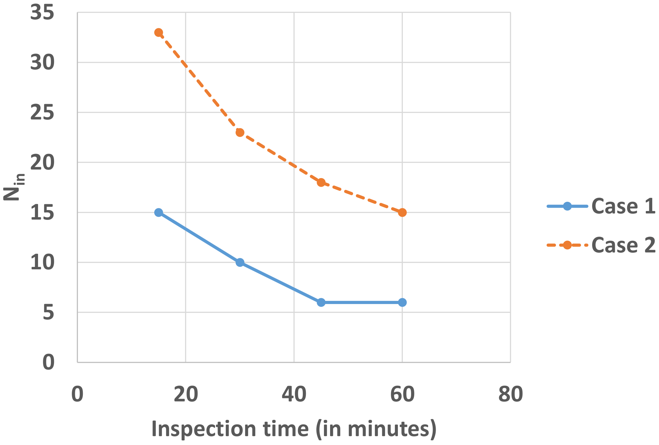
• A time of 30 min devoted to inspections and their interpretation
• Immobilization inducing a loss of 2 h, including staff as well as users in the event of failure and corrective maintenance
• A churn rate of 1% linked to the loss of users in the event of failure
• A perfect ability of the drowsiness detector to avoid accidents related to it

A cost function is constructed, including risks, both human and financial. Two theoretical methods allow for a monetized evaluation of the risks. First, the usual perspectives based on a multiplicative conception of probabilities and consequences or their monetary equivalents. On the other hand, we also rely on the current of Prospect Theory initiated by Kahneman and Tversky, based on a distortion of probabilities as consequences, amplifying the evaluation of consequences for low probability risks (especially human risks).

Thus, when we compare the results obtained according to the two methods, the maintenance optima are clearly different. If the optimal number of inspections is 10 in the base case for a linear valuation perspective, it is 23 when the theoretical valuation path is that of Prospect Theory. The monetary equivalent including both maintenance costs and risk assessment—financial and human—is then (when optimal maintenance is achieved) €595 in the first case and €1332 in the second one. As the risks relating to a failure are evaluated more intensely, it is very consistent to favor greater safety and more frequent inspections. Several key parameters about which uncertainties remain are the subject of a sensitivity analysis.

5.1. Variation of the Churn Rate

If the base case is based on a loss of turnover of 1% linked to the loss of users in the event of failure, we consider a variation between 1% and 10%. Indeed, little is precisely known about the purchasing behavior of consumers in the event of an accident – apart from humanly serious cases. This behavior depends on the structure of the transport market, the alternatives available to users and the consequences of failures, particularly in terms of lost time. The variations considered are therefore within the ranges usually observed during incidents on a transport network.

Over the range of variation between 1% and 10%, the optimal number of inspections increases from 10 to 19 in the linear case and from 23 to 36 by mobilizing Prospect Theory. Along this same range, the minimum cost including risks goes from €595 to €987 and from €1332 to €2023, respectively. Within these generalized costs, the proportion of financial risks increases from 12 to 30% for the linear method and from 11 to 31% for Prospect Theory (Figure 5). Such results are consistent as far as the increase in the churn rate leads, whatever the method, to an amplification of financial risks, of aggregated monetary equivalents, thus making inspections more necessary to minimize risks.

5.2. Variation of Inspection Time

If initially, a time of 30 min was considered for each inspection and its interpretation, we also consider the possibility of a variation in this time between 15 min and 1 h (15 min, 45 min and 1 h) for the same hourly cost of 60€. Quite logically, a faster inspection—less expensive—makes inspections more frequent, going from an optimal number of 10 to 15 in the linear case and from 23 to 33 by mobilizing Prospect Theory. In this change, the minimum cost including the risks goes, respectively, from €595 to €416 and from €1332 to €927. Similarly, a longer inspection makes inspections less frequent, going from an optimal number of 10 to 6 in the linear case and from 23 to 18 when mobilizing Prospect Theory. With such a variation, the minimum cost including the risks goes, respectively, from €595 to €720 and from €1332 to €1641. Finally, an inspection and interpretation time of up to 1 h makes inspections even less frequent, again going from an optimal number of 10 to 6 in the linear case (compared to the base case) and from 23 to 15 in mobilizing Prospect Theory (Figure 6). In this evolution compared to the initial case, the minimum cost including the risks goes, respectively, from €595 to €810 and from €1332 to €1897.

5.3. Variation of Operational Losses

If initially, an immobilization period of 2 h was considered, basing the calculation of operational losses, we also consider the possibility of a variation in this time between 1 h and 5 h (1 h, 3 h, 4 h and 5 h) for the same hourly cost. Quite logically, a shorter—less expensive—downtime of one hour makes inspections less frequent, going from an optimal number of 10 to 9 in the linear case and remaining at 23 by mobilizing Prospect Theory. In this new context, the minimum cost including the risks goes from €595 to €567 and from €1332 to €1324, respectively. Similarly, a longer immobilization makes inspections more frequent, going for 3 h of immobilization from an optimal number of 10 to 11 and remaining at 23 by mobilizing Prospect Theory. With such an evolution, the minimum cost including risks goes from €595 to €622 and from €1332 to €1341, respectively. Similarly, a 4 h immobilization leads to, respectively, 11 and 23 inspections at the optimum. The minimum cost including the risks goes from €595 to €645 and from €1332 to €1349, respectively. Finally, an immobilization period of up to 5 h can still change the situation with an optimal number of inspections being, respectively, 12 and 23 according to the linear approach or that of Prospect Theory. Compared to the initial case, the minimum cost including the risks goes, respectively, from €595 to €668 and from €1332 to €1357 (Figure 7).

The stability of the inspections carried out when the optimization is based on the second method actually comes from the fact that the amounts associated with operational losses are low compared to the assessment of the risks, in particular human risks, for a high number of inspections. Thus, the trade-offs and the optimal number of inspections are not modified. The variations are quite small even with linear approach. However, the slightly higher number of operational losses for fewer inspections (in the case of a linear approach) as well as the lower risk assessment can change slightly the situation and the trade-offs, thus modifying the number of inspections (Figure 7).

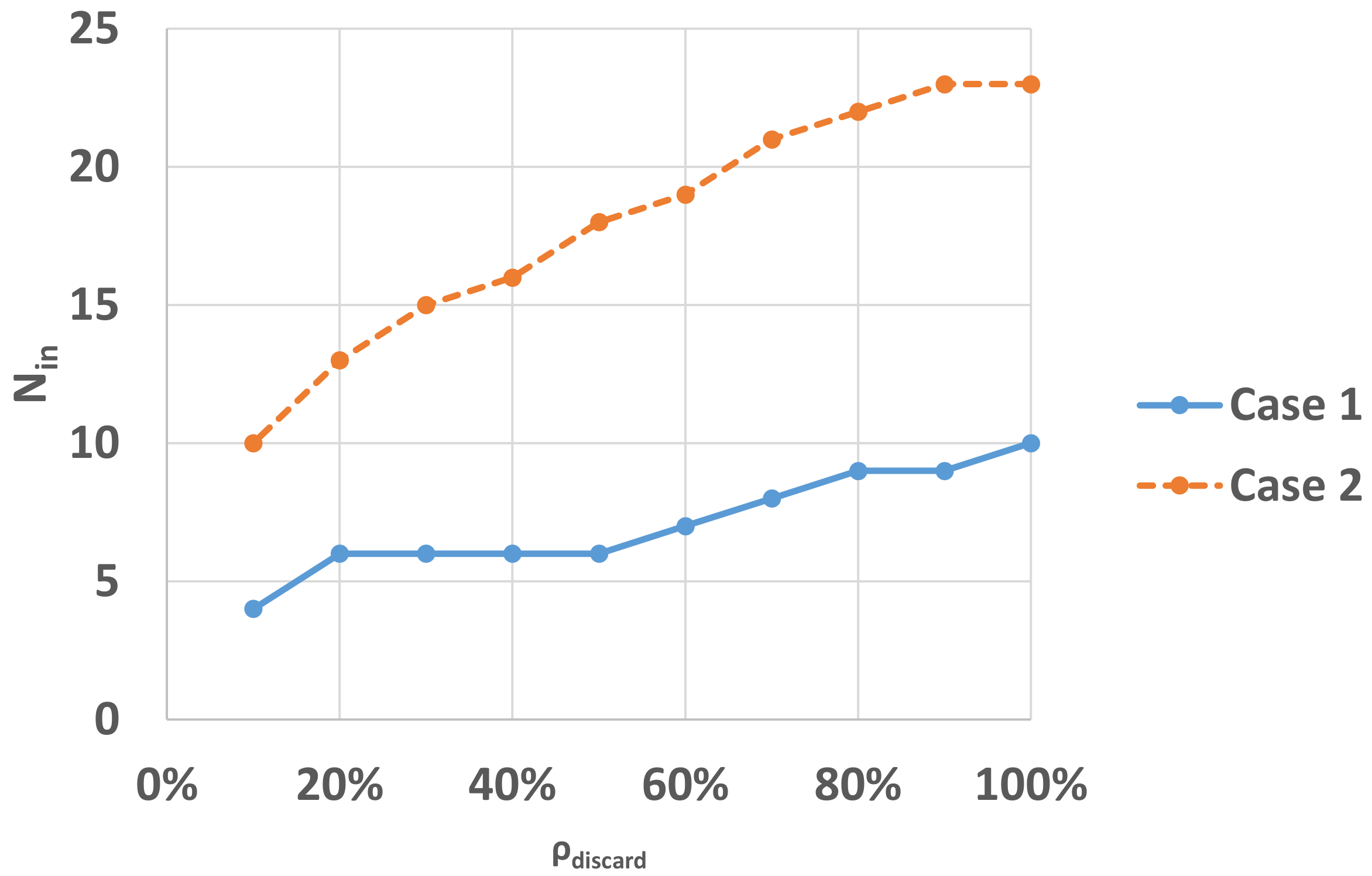
5.4. Variation of the Discard Rate

Initially, we considered ${\rho }_{discard}=100\%$, meaning the system is able to detect and treat $100\%$ of drowsiness situations. Then, we considered the possibility of variation of ${\rho }_{discard}$ from $10\%$ to $100\%$. Quite logically, high values of ${\rho }_{discard}$ lead to high values of financial and human risks as the system is considered to be efficient in treating drowsiness situations. This leads systematically to high number of inspections. In the considered case study, a variation of ${\rho }_{discard}$ from $10\%$ to $100\%$ leads to a variation of the optimal $C_{tot}$ from €359.25 to €595.43 and a variation of the optimal $N_{in}$ from 4 to 10 according to the linear approach. However, a variation of ${\rho }_{discard}$ from $10\%$ to $100\%$ leads to a variation of the optimal $C_{tot}$ from €675.18 to €1332.42 and a variation of the optimal $N_{in}$ from 10 to 23 according to Prospect Theory (Figure 8). We notice a more accentuated variation of the optimal $N_{in}$ in the case of Prospect Theory than in the linear approach. This can be explained by a risk aversion behavior that tends to increase inspections as risks become more important. This risk aversion is also shown in the optimal number of inspections for ${\rho }_{discard}=10\%$ which is equal to 10 in the case of prospect theory, a result that is comparable to the optimal number of inspections for ${\rho }_{discard}=100\%$ in the linear approach. This means that a decision maker who is risk-averse will remain so regardless of the effectiveness of the system to detect and treat drowsiness situations (Figure 8).

6. Conclusions

The method for maintenance cost optimization that we propose in this paper does not only consider direct costs of maintenance but also risks in the case of system failure. The process of human decision making is primordial in PdM optimization. This aspect has been considered by applying prospect theory in the evaluation of maintenance risks. Prospect theory illustrated the impact of the human psychology on the risk evaluation: people tend generally to overestimate low probabilities meaning that people are over concerned with the outcome of the probability rather than the probability itself when it comes to deal with low probabilities of risks. It has also alleviated the framing effect where people generally decide on options based on whether the options are presented as losses or gains, by setting a reference point according to which losses and gains are defined.

The output of the optimization methodology described in this paper depends on the input parameters (time and cost parameters). Carrying out a sensitivity analysis will allow determining the most influencing input parameters. Some reflections on how to handle these input parameters can be drawn from this sensitivity analysis in order to help experts better improve the results of the proposed optimization methodology.

In reality, a component is interconnected with other components and a failure in a component may lead to a dysfunction in other components. Therefore, this methodology for maintenance cost optimization needs to be extended to deal with complex systems with interconnected components. Moreover, the parameters used in the valuation and probability transformation function are estimated statistically following several empirical experiences done on human subjects. The question arises as to what extent these parameters are dependent on the context of study.

References

1. UNE EN 13306:2018 AFNOR; Maintenance Terminology. European Standard: Pilsen, Czech Republic, 2018.
2. Ran, Y.; Zhou, X.; Lin, P.; Wen, Y.; Deng, R. A survey of predictive maintenance: Systems, purposes and approaches. arXiv 2019, arXiv:1912.07383. [Google Scholar]
3. Ly, C.; Tom, K.; Byington, C.S.; Patrick, R.; Vachtsevanos, G.J. Fault diagnosis and failure prognosis for engineering systems: A global perspective. In Proceedings of the 2009 IEEE International Conference on Automation Science and Engineering, Bangalore, India, 22–25 August 2009; pp. 108–115. [Google Scholar]
4. Banjevic, D. Remaining useful life in theory and practice. Metrika 2009, 69, 337–349. [Google Scholar] [CrossRef]
5. Si, X.S.; Wang, W.; Hu, C.H.; Zhou, D.H. Remaining useful life estimation—A review on the statistical data driven approaches. Eur. J. Oper. Res. 2011, 213, 1–14. [Google Scholar] [CrossRef]
6. Okoh, C.; Roy, R.; Mehnen, J.; Redding, L. Overview of remaining useful life prediction techniques in through-life engineering services. Procedia Cirp. 2014, 16, 158–163. [Google Scholar] [CrossRef] [Green Version]
7. Khan, F.I.; Haddara, M.M. Risk-based maintenance (RBM): A quantitative approach for maintenance/inspection scheduling and planning. J. Loss Prev. Process. Ind. 2003, 16, 561–573. [Google Scholar] [CrossRef]
8. Louhichi, R.; Sallak, M.; Pelletan, J. A cost model for predictive maintenance based on risk-assessment. In Proceedings of the 13th Conférence Internationale CIGI QUALITA, Montreal, QC, Canada, 25 June 2019. [Google Scholar]
9. Kahneman, D. Prospect theory: An analysis of decisions under risk. Econometrica 1979, 47, 278. [Google Scholar] [CrossRef] [Green Version]
10. Allais, M. Le comportement de l’homme rationnel devant le risque: Critique des postulats et axiomes de l’école américaine. Econom. J. Econom. Soc. 1953, 21, 503–546. [Google Scholar] [CrossRef] [Green Version]
11. Pelletan, J. Fondements Économiques d’une Politique de Sécurité: L’Exemple du Risque de Criminalité. Economics Thesis, University Paris Dauphine, Paris, France, 2008. [Google Scholar]
12. Louhichi, R. Élaboration d’un Modèle Économique Optimisant la Stratégie de Maintenance. Ph.D. Thesis, Université de Technologie de Compiègne, Compiègne, France, 2021. [Google Scholar]
13. Hewes, D.E.; Kahneman, D.; Slovic, P.; Tversky, A. Judgement under uncertainty: Heuristics and biases. J. Commun. 1983, 33, 21–22. [Google Scholar]
14. Tversky, A.; Koehler, D. Support theory: A nonextensional representation of subjective probability. Psychol. Rev. 1994, 101, 547–567. [Google Scholar] [CrossRef]
15. Cheng, M.; Frangopol, D.M. Life-cycle optimization of structural systems based on cumulative prospect theory: Effects of the reference point and risk attitudes. Reliab. Eng. Syst. Saf. 2022, 218, 108100. [Google Scholar] [CrossRef]
16. Gong, C.; Frangopol, D.M.; Cheng, M. Application of Cumulative Prospect Theory to Optimal Inspection Decision-Making for Ship Structures. In Model Validation and Uncertainty Quantification, Volume 3. Conference Proceedings of the Society for Experimental Mechanics Series; Barthorpe, R., Ed.; Springer: Cham, Switzerland, 2020. [Google Scholar]
17. Louhichi, R.; Sallak, M.; Pelletan, J. A maintenance cost optimization approach: Application on a mechanical bearing system. Int. J. Mech. Eng. Robot. Res. 2020, 9, 658–664. [Google Scholar] [CrossRef]
18. Zeller, O. L’historien et Les Risques Industriels: Récente Émergence d’une Curiosité. Fondation Pour une Culture de Sécurité Industrielle; FONCSI: Toulouse, France, 2015. [Google Scholar]
19. Louhichi, R.; Sallak, M.; Pelletan, J. Avenues for future research on predictive maintenance purposes in terms of risk minimization. In Proceedings of the European Safety and Reliability Conference (ESREL), Venice, Italy, 21–26 June 2020. [Google Scholar]
20. Zio, E. The future of risk assessment. Reliab. Eng. Syst. Saf. 2018, 177, 176–190. [Google Scholar] [CrossRef]
21. Aven, T. Risk Analysis; John Wiley & Sons: Hoboken, NJ, USA, 2015. [Google Scholar]
22. Krishnasamy, L.; Khan, F.; Haddara, M. Development of a risk-based maintenance (RBM) strategy for a power-generating plant. J. Loss Prev. Process. 2005, 18, 69–81. [Google Scholar] [CrossRef]
23. Bertolini, M.; Bevilacqua, M.; Ciarapica, F.E.; Giacchetta, G. Development of risk-based inspection and maintenance procedures for an oil refinery. J. Loss Prev. Process. Ind. 2009, 22, 244–253. [Google Scholar] [CrossRef]
24. Leoni, L.; BahooToroody, A.; De Carlo, F.; Paltrinieri, N. Developing a risk-based maintenance model for a Natural Gas Regulating and Metering Station using Bayesian Network. J. Loss Prev. Process. Ind. 2019, 57, 17–24. [Google Scholar] [CrossRef]
25. Kao, C.S.; Hu, K.H. Acrylic reactor runaway and explosion accident analysis. J. Loss Prev. Process. 2002, 15, 213–222. [Google Scholar] [CrossRef]
26. Yazdi, M.; Korhan, O.; Daneshvar, S. Application of fuzzy fault tree analysis based on modified fuzzy AHP and fuzzy TOPSIS for fire and explosion in the process industry. Int. J. Occup. Ergon. 2020, 26, 319–335. [Google Scholar] [CrossRef]
27. Dionne, G.; Lebeau, M. Le calcul de la valeur statistique d’une vie humaine. Actual. Écon. 2010, 86, 487–530. [Google Scholar] [CrossRef] [Green Version]
28. Dionne, G.; Lanoie, P. Public choice about the value of a statistical life for cost-benefit analyses: The case of road safety. J. Transp. Econ. Policy (JTEP) 2004, 38, 247–274. [Google Scholar]
29. Lanoie, P.; Pedro, C.; Latour, R. The value of a statistical life: A comparison of two approaches. J. Risk Uncertain. 1995, 10, 235–257. [Google Scholar] [CrossRef]
30. Handbook of the Economics of Risk and Uncertainty; Machina, M.; Viscusi, W.K. (Eds.) Elsevier: Amsterdam, The Netherlands, 2013. [Google Scholar]
31. Commissariat Général à la Stratégie et à La Prospective Département Dévelopement Durable. Éléments Pour Une Révision de La Valeur de La vie Humaine; République Française: Paris, France, 2013. [Google Scholar]
32. Commissariat Général à la Stratégie et à la Prospective. Eléments Pour une Révision de la Valeur Statistique de la vie Humaine; Public Report; France Stratégie: Paris, France, 2013. [Google Scholar]
33. Quinet, E. Commissariat Général à la Stratégie et à la Prospective. L’évaluation Socioéconomique des Investissements Publics; Public Report; France Stratégie: Paris, France, 2013; p. 105. [Google Scholar]
34. Ngobo, P.V.; Ramaroson, A. Facteurs déterminants de la relation entre la satisfaction des clients et la performance de l’entreprise. Décis. Mark. 2005, 40, 75–84. [Google Scholar] [CrossRef]
35. Crie, D. Rétention de clientèle et fidélité des clients. Décis. Mark. 1996, 7, 25–30. [Google Scholar] [CrossRef]
36. Gao, T.; Wang, X.C.; Chen, R.; Ngo, H.H.; Guo, W. Disability adjusted life year (DALY): A useful tool for quantitative assessment of environmental pollution. Sci. Total Environ. 2015, 511, 268–287. [Google Scholar] [CrossRef] [PubMed]
37. Salomon, J.A. Techniques for valuing health states. Encycl. Health Econ. 2014, 2, 454–458. [Google Scholar]
38. Prüss-Üstün, A.; Mathers, C.; Corvalán, C.; Woodward, A. Introduction and Methods: Assessing the Environmental Burden of Disease at National and Local Levels; World Health Organization: Geneva, Switzerland, 2003. [Google Scholar]
39. Holland, M.; Pye, S. Damages per Tonne Emission of EU25 Member State (Excluding Cyprus) and Surrounding Sea Service Contract for Carrying Out Cost-Benefit Analysis of Air Quality Related Issues, in Particular in the Clean Air for Europe (CAFE) Programme Customer; AEA Technology Environment: Oxfordshire, UK, 2005. [Google Scholar]
40. Dehghani, N.L.; Darestani, Y.M.; Shafieezadeh, A. Optimal life-cycle resilience enhancement of aging power distribution systems: A MINLP-based preventive maintenance planning. IEEE Access 2020, 8, 22324–22334. [Google Scholar] [CrossRef]
41. Yazdi, M.; Nedjati, A.; Abbassi, R. Fuzzy dynamic risk-based maintenance investment optimization for offshore process facilities. J. Loss Prev. Process. Ind. 2019, 57, 194–207. [Google Scholar] [CrossRef]
42. Von Neumann, J.; Morgenstern, O. Theory of Games and Economic Behavior. In Theory of Games and Economic Behavior; Princeton University Press: Princeton, NJ, USA, 2007. [Google Scholar]
43. Morgenstern, O. The collaboration between Oskar Morgenstern and John von Neumann on the theory of games. J. Econ. Lit. 1976, 14, 805–816. [Google Scholar]
44. Camerer, C.F.; Ho, T.H. Nonlinear weighting of probabilities and violations of the betweenness axiom. J. Risk Uncertain. 1994, 8, 167–196. [Google Scholar] [CrossRef]
45. Kachelmeier, S.J.; Shehata, M. Examining Risk Preferences under High Monetary Incentives Experimental Evidence from the People’s Republic of China. Am. Econ. Rev. 1992, 82, 1120–1141. [Google Scholar]
46. Abdellaoui, M. Parameter-Free Elicitation of Utility and Probability Weighting Functions. Manag. Sci. 2000, 46, 1497–1512. [Google Scholar] [CrossRef]
47. Abdellaoui, M.; Vossmann, F.; Weber, M. Choice-based Elicitation and Decomposition of Decision Weights for Gains and Losses under Uncertainty. Manag. Sci. 2005, 51, 1384–1399. [Google Scholar] [CrossRef] [Green Version]
48. Wu, G.; Gonzalez, R. Curvature of the Probability Weighting Function. Manag. Sci. 1996, 42, 1676–1690. [Google Scholar] [CrossRef] [Green Version]
49. Bleichrodt, H.; Pinto, J.L. A Parameter-Free Elicitation of the Probability Weighting Function in Medical Decision Analysis. Manag. Sci. 2000, 46, 1485–1496. [Google Scholar] [CrossRef]
50. Rajasekar, R.; Pattni, V.B.; Vanangamudi, S. Drowsy Driver Sleeping Device and Driver Alert System. Int. J. Sci. Res. 2014, 3, 2319–7064. [Google Scholar]
51. Subbarao, A.; Sahithya, K. Driver drowsiness detection system for vehicle safety. Int. J. Innov. Technol. Explor. Eng. (IJITEE) 2010, 8, 815–819. [Google Scholar]
52. Danisman, T.; Bilasco, I.M.; Djeraba, C.; Ihaddadene, N. Drowsy driver detection system using eye blink patterns. In Proceedings of the 2010 IEEE International Conference on Machine and Web Intelligence, Algiers, Algeria, 3–5 October 2010; pp. 230–233. [Google Scholar]
53. Erto, P. New practical Bayes estimators for the 2-parameter Weibull distribution. IEEE Trans. Reliab. 1982, 31, 194–197. [Google Scholar] [CrossRef]
54. Erto, P.; Giorgio, M. A note on using Bayes priors for Weibull distribution. arXiv 2013, arXiv:1310.7056. [Google Scholar]
55. Nuyttens, N.; Stipdonk, H.; Van Schagen, I. Dossier Thématique Sécurité Routière no. 15. Les Blessés de la Route et Leurs Lésions; Vias Insitute—Centre de Connaissance Sécurité Routière: Brussels, Belgium, 2018. [Google Scholar]
56. European Commission. Mobility and Transport, Road Safety; Road Safety Facts and Figures; Public Report from European Commission; European Commission: Brussels, Belgium, 2018. [Google Scholar]
57. Association Hello Victimes. Barèmes d’Indemnisation et Référentiels Indicatifs Actualisés des Courts d’Appel. Association Hello Victimes. 2018. Available online: https://www.hello-victimes.fr/ (accessed on 8 October 2020).
58. Ministère de la Transition Écologique. Le Transport Collectif Routier de Voyageurs en 2015: Circulation et Parc en Progression, Parcours Moyen Stable; Public Report; Ministère de la Transition Écologique: Paris, France, 2016. [Google Scholar]
Figure 1. Main typologies for cost/risk minimization in maintenance [19].
Applsci 12 11748 g001
Figure 2. Valuation function.
Applsci 12 11748 g002
Figure 3. Probability transformation function.
Applsci 12 11748 g003
Figure 4. Eye blink sensor [51,52].
Applsci 12 11748 g004
Figure 5. Variation of the optimal N i n in terms of the churn rate y: case 1 versus case 2.
Applsci 12 11748 g005
Figure 6. Variation of the optimal N i n in terms of inspection time: case 1 vs. case 2.
Applsci 12 11748 g006
Figure 7. Variation of the optimal N i n in terms of period of system immobilization for maintenance: case 1 vs. case 2.
Applsci 12 11748 g007
Figure 8. Variation of the optimal N i n in terms of the discard rate: case 1 vs. case 2.
Applsci 12 11748 g008