Abstract
MR scans of low-gamma X-nuclei, low-concentration metabolites, or standard imaging at very low field entail a challenging tradeoff between resolution, signal-to-noise, and acquisition duration. Deep learning (DL) techniques, such as UNets, can potentially be used to improve such “low-quality” (LQ) images. We investigate three UNets for upscaling LQ MRI: dense (DUNet), robust (RUNet), and anisotropic (AUNet). These were evaluated for two acquisition scenarios. In the same-subject High-Quality Complementary Priors (HQCP) scenario, an LQ and a high quality (HQ) image are collected and both LQ and HQ were inputs to the UNets. In the No Complementary Priors (NoCP) scenario, only the LQ images are collected and used as the sole input to the UNets. To address the lack of same-subject LQ and HQ images, we added data from the OASIS-1 database. The UNets were tested in upscaling 1/8, 1/4, and 1/2 undersampled images for both scenarios. As manifested by non-statically significant differences of matrices, also supported by subjective observation, the three UNets upscaled images equally well. This was in contrast to mixed effects statistics that clearly illustrated significant differences. Observations suggest that the detailed architecture of these UNets may not play a critical role. As expected, HQCP substantially improves upscaling with any of the UNets. The outcomes support the notion that DL methods may have merit as an integral part of integrated holistic approaches in advancing special MRI acquisitions; however, primary attention should be paid to the foundational step of such approaches, i.e., the actual data collected.
1. Introduction
While MRI is a powerful modality, its low sensitivity, inherent to the nuclear magnetic resonance phenomenon, results in a practical tradeoff between spatial resolution, signal-to-noise ratio (SNR), and acquisition duration [1,2,3,4]. A host of innovative and groundbreaking techniques have been introduced to optimize this tradeoff. For example, undersampling portions of k-space [5], compressed sensing [6], and parallel imaging [7,8] enable a reduction of the acquisition time without substantial loss in SNR and spatial resolution. However, when SNR is low, this tradeoff shifts towards increased acquisition duration and/or larger voxel sizes. Such examples are the case for chemical shift imaging (CSI), especially of low-concentration molecular species [9], imaging at low main magnetic fields [10], and X-nuclei MRI [11]. To improve such low-resolution and low-SNR images, denoted as “low quality” (LQ) from now on, various methods have been introduced, such as multiple- and single-image super-resolution reconstruction [12,13,14,15,16], density-weighted k-space scanning [17], and denoising techniques applied to both the spatial and k-space domains [18,19,20].
To enhance the range of options in managing the aforementioned tradeoffs and improving LQ MRI, investigators have pursued deep learning (DL) methods including U-Net convolutional networks [21,22,23,24,25,26,27,28], MRI-specific DL architectures [29], and generative adversarial networks (GANs) [13,30,31,32]. The inputs to these trained networks are the physically collected LQ MR data and the output is a higher resolution and/or higher SNR image; a high quality (HQ) MRI. Motivated by the potential benefit of using DL to upscale low main magnetic field [21,22,23,24,25,26,27] and X-nuclei MRI, we first evaluated UNets, a robust performer in medical image segmentation [33,34,35,36,37,38], as well as having shown its utility in upscaling MR data, such as CSI [21], diffusion weighted imaging [26] and real time imaging [39]. The versatile and widely used state-of-the-art UNet offers a simple and intuitive neural network framework, originally designed for image segmentation, which can be modified to include and link substantially different operations and functions. Examples of UNet architectural modifications include work that uses double convolutions, dense connections, residual addition, and pixel shuffle, to improve the quality of diffusion weighted MRI [26], or substitute the max-pool with an average pooling layer [25]. Other works have further explored the UNet framework, such as Ding et al., who used global residual to enhance the quality of images in [27], while Nasrin et al. used a residual architecture in UNet to enhance resolution and denoise medical images in [28]. This diversity enables high versatility in capturing context or features [33] in the input LQ images and then combines spatial and contextual information to generate the output HQ image.
Secondary to the established performance of UNets, there is an ever-growing number of U-Net architectural modifications that exhibit good performances for the tested datasets and employed metrics [21,22,23,24,25,26,27,28,33,34]. With such a great number of UNet variants, it becomes increasingly challenging to identify the most useful architecture and/or training pipeline. Interestingly, a recent study has also pointed to the importance of loss functions as compared to architectural modifications [40]. These observations led us to the present study, which focuses on aspects of the performance of three UNet architectures on upscaling LQ MRI: a dense (DUNet) [21], a robust (RUNet) [22], and an anisotropic (AUNet) [23]. These were selected since, firstly, they have previously been explored for improving LQ MRI, and secondly, they have quite different architectural layers, which is a starting point in assessing the differential benefit of such architectural modifications.
Within this context, our contribution involves comparing these three UNets in upscaling LQ MRI for different acquisition scenarios, for the same training and performance-testing datasets as well as the same training conditions. Specifically, to replicate practical acquisition scenarios, the three UNets were tested on (a) two image acquisition scenarios and (b) for three different acquisition matrices. In one case, herein referred to as With-Priors, we replicated an imaging protocol that collects LQ as well as a same-subject high quality complementary prior (HQCP) image that is of different contrast, finer spatial resolution, and higher SNR. Examples of this acquisition scenario include LQ 23Na MRI [41] or CSI [9] images collected together with the HQ 1H anatomical scans. In the other acquisition scenario, herein referred to as WithOut-Priors, only the LQ data set is collected during an imaging session: this would be the case, for example, for low magnetic field MRI [10,42]. The three UNets for the two acquisition scenarios (i.e., six cases of scenarios/Unet pairs) were trained and tested for upscaling LQ images collected with different acquisition matrices (i.e., spatial resolutions) of 1/8, 1/4, and 1/2 of the matrix size of the targeted upscaled reconstructed image. To analyze the reconstructed images of the three Unets we used Mean Squared Error (MSE) and Structural Similarity Index Measure (SSIM), Peak Signal to Noise Ratio (PSNR), and Mean Intensity Error (MIE). Yet another contribution of this work is the analysis of the significance of the three Unet architectures, the three acquisition matrices, and the two acquisition scenarios, not just by descriptive statistics (i.e., means and standard deviations), but with mixed effects (aka repeated measures) modeling (MEM) [43]. MEM analysis was selected, as it takes into account that in this study we performed repeated measurements (i.e., multiple evaluation measurements) on a set of distinct images. For the MEM analysis, the fixed effects were determined by the type of UNet (with three levels), and the matrix size (also with three levels) along with their interaction, while the images constitute the random effects.
Our main contributions stem from the thorough comparison of the three state-of-the-art UNet architectures that entail:
- Two different acquisition scenarios: (a) the With-Priors that mimic studies that entail the collection of both an LQ image and its complementary high quality prior to upscale the image to a corresponding HQ target, (b) the WithOut-Priors that mimic studies that entail the collection of only a single LQ Image to upscale the image to a corresponding HQ target.
- Creation of synthetic training and testing data so we have the same set of LQ images, its complementary HQ prior, and an HQ image (ground truth). In addition, hyperintense lesions of random intensity, size, and position were added to increase the variability in the images.
- The collected LQ Images were truncated to three smaller matrix sizes to mimic studies where the acquisition matrix sizes are small. We train the networks to upscale these images in two acquisition scenarios.
- An extensive analysis of the quality of the upscaled images obtained from different UNet was performed using various indices and statistical tests using a mixed effects model.
2. Materials and Methods
2.1. Training and Testing Dataset
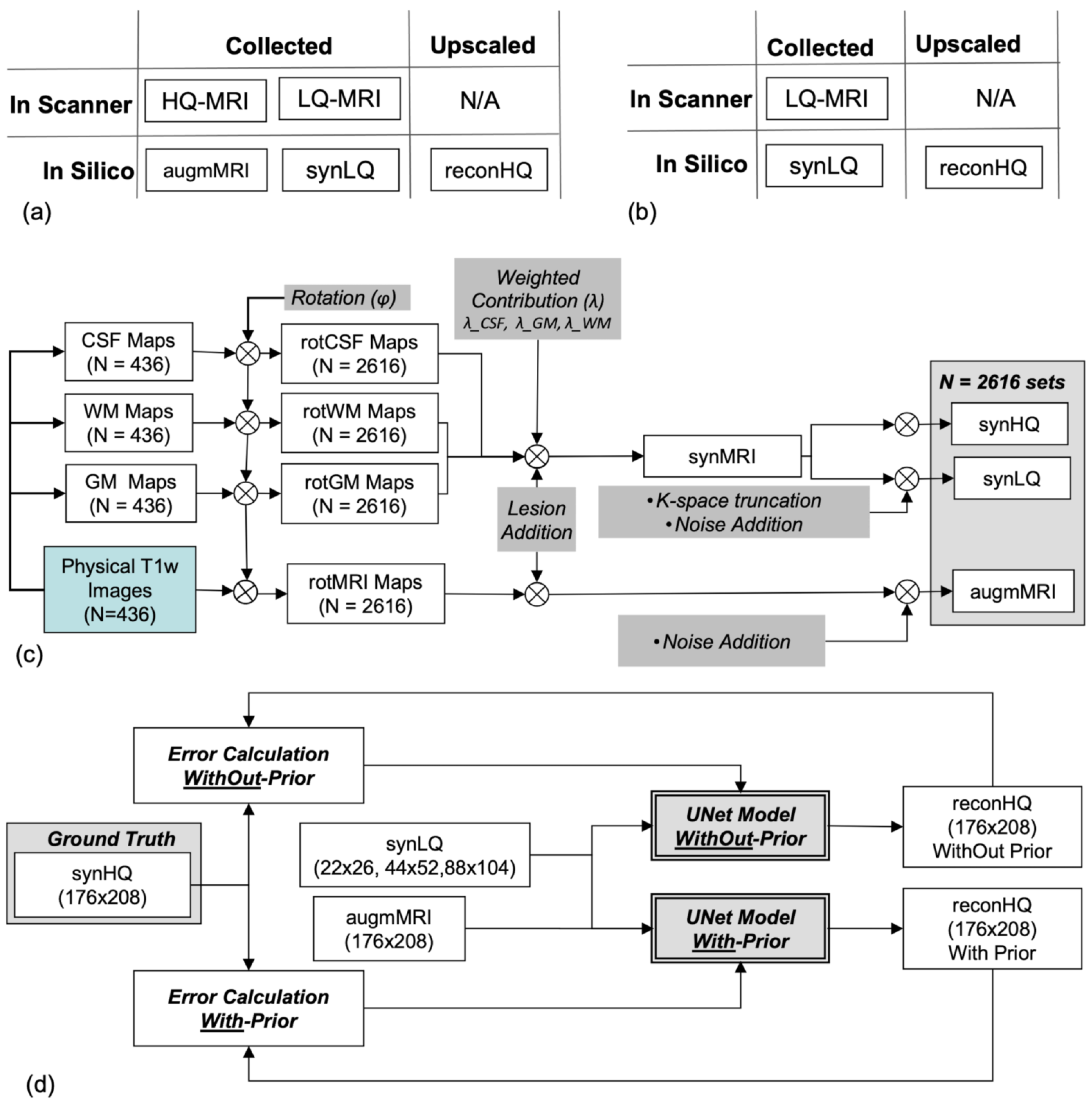
In silico LQ-to-HQ UNet upscaling studies require the networks to be trained and tested with spatially/anatomically matched pairs of LQ and HQ images (i.e., of the same structures). As such matched datasets are not publicly available and are difficult to collect, we synthesized them from publicly accessible images, a commonly used practice in DL [44,45,46,47,48], to increase the size and variability in training and testing data. As illustrated in Figure 1a,b, evaluation of the UNets for the two scanning scenarios require matching sets from the same object consisting of: (i) an LQ (input) and an HQ (ground truth) for the WithOut-Prior, and (ii) an LQ and an HQCP image (the two inputs) and an HQ (ground truth) for the With-Prior. The three UNets were trained and tested for the two acquisition scenarios using synthetic imaging data as has been the practice in numerous prior works.
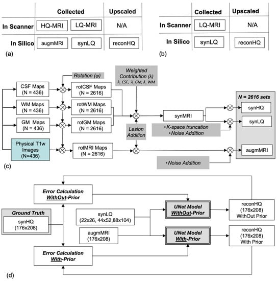
Figure 1.
(a,b) Illustrations of the two paradigms With-Prior (a) and WithOut-Prior (b) (i.e., same-subject complementary high resolution images collected at the same location), showing the type of data collected on the scanner and generated in silico. (c) Flowchart of the processes employed in the generation of 2616 data sets that included high quality synthetic (synHQ), low quality synthetic (synLQ), and augmented physically collected T1-weighted (augmMRI) images. (d) Flowchart of the UNet training to upscale the synLQ to synHQ, for the two paradigms of With- and WithOut-Prior; in the first case, the augmMRI served as the high quality complementary prior.
The synthetic data were composed of 2616 image sets; of these, 2076 were used for training and 540 for testing; the split in training/testing was performed at random. This data set was synthesized from 436 actual MRI images obtained from the OASIS project [49], which were augmented to a total number of 2616 using a customized image generator based on the one reported by Iqbal et al. [21] and modified to include structural, noise, and signal intensity variations. As illustrated in Figure 1c, we started with 436 data sets from the OASIS project [49] with each set containing a 176 × 208 T1-weighted brain image (used as HQCP) together with the corresponding segmented binary maps of cerebrospinal fluid (CSF), white (WM), and gray matter (GM). Our data augmentation processes first included subjecting each data set, i.e., the T1-weighted image (HQCP Image) and the GW, WM, and CSF maps, to six random rotations, resulting in 2616 sets of 176 × 208 rotMRI, rotGM, rotWM, and rotCSF, respectively. Then, hyperintense lesions of circular shape with random size and position followed by an elastic deformation [33,34] were added to the WM and GM regions. Various techniques have been introduced that can enhance the lesions in the brain as described by Mzoughi et al. [50] and Kleesiek et al. [51]. This image enhancement can also be performed at the acquisition level by using gadolinium-based contrast agents [51].
Since elastic deformation was used and lesions were restricted to the WM and GM the lesions had random shapes and sizes. Each rotMRI was further modified by adding 5% Gaussian noise and this image was designated as the augmMRI serving as the HQCP to the training of the With-Prior acquisition scenario. rotWM, rotGM, and rotCSF were combined using random weighting factor to produce synthetic MRI (synMRI) images with a digital resolution of 176 × 208. The 176 × 208 synMRI images were designated as the denoised high-quality synthetic (synHQ) images that served as the Ground Truth, as well as being used to generate all low-quality synthetic (synLQ) images by first combining CSF, GM, and WM images with random weighting individual factors between 0.9 and 1.1, followed by adding 20% Gaussian noise and then downsampling by k-space truncation to the 1/8 (22 × 26), 1/4 (44 × 52), and 1/2 (88 × 104) of the full k-space acquisition matrix of the original OASIS T1-weighted images [49]. The outcomes of data synthesis were 2616 data sets, each composed of a 176 × 208 augmMRI (i.e., the HQCP), a 176 × 208 synHQ (i.e., the Ground Truth for this set), and three LQ (lower resolution and noisy) synthetic images, a 22 × 26 synLQ, a 44 × 52 synLQ, and an 88 × 104 synLQ. All the synLQ images were interpolated to the original OASIS images matrix size using nearest neighbor interpolation before being used as inputs to the networks. Nearest neighbor interpolation was used to preserve the distribution of the image
The obtained datasets were then used in the two different processing scenarios. Experiment 1 uses the augmMRI and the synLQ images as inputs, and the synHQ image as the ground truth for reconstruction. Experiment 2 uses only the synLQ images as input, and the synHQ images as ground truth for reconstruction. The obtained dataset of 416 patients 80% training based on (332 patients leading to 2076 images) data and 20% testing data (84 patients, leading to 540 images). The training data are further divided into 80% training (1661 images) and 20% validation (415 images) data.
2.2. UNet Architectures
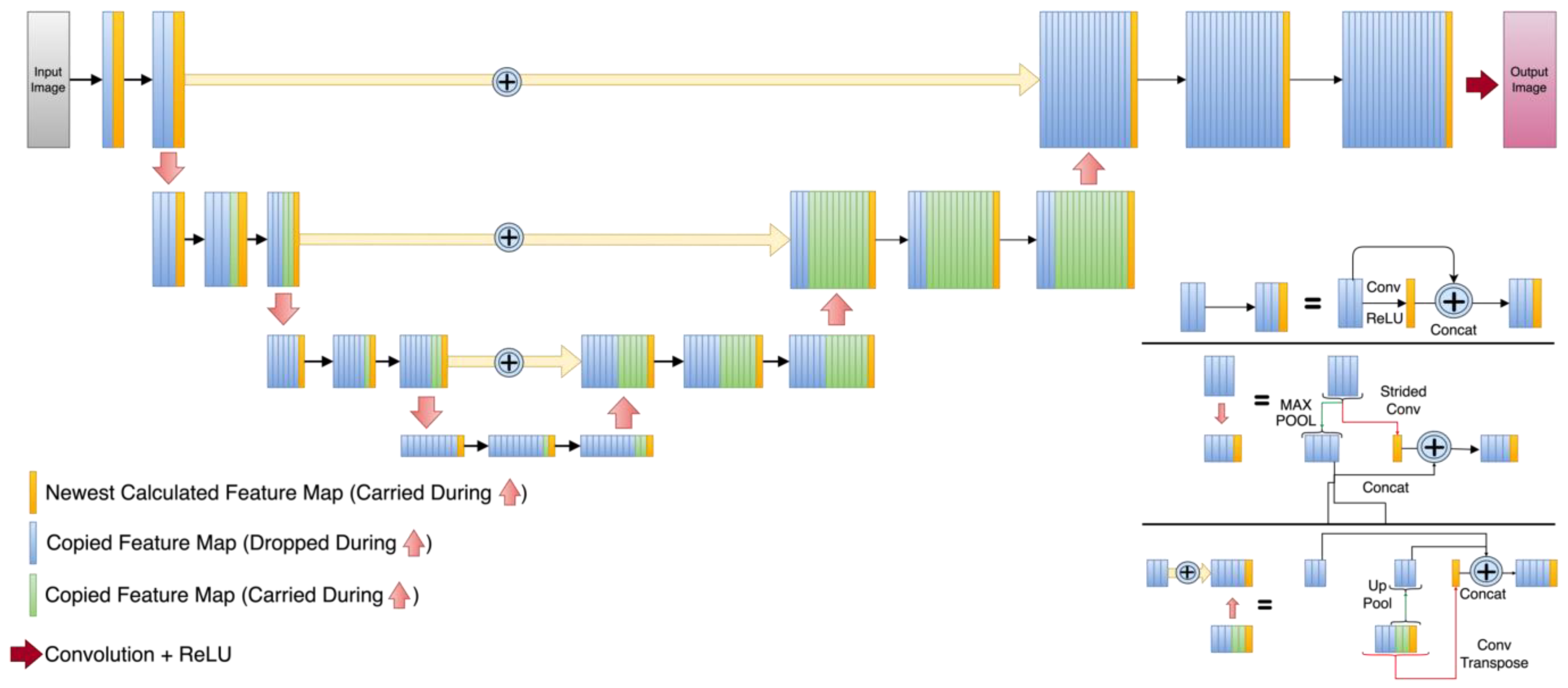
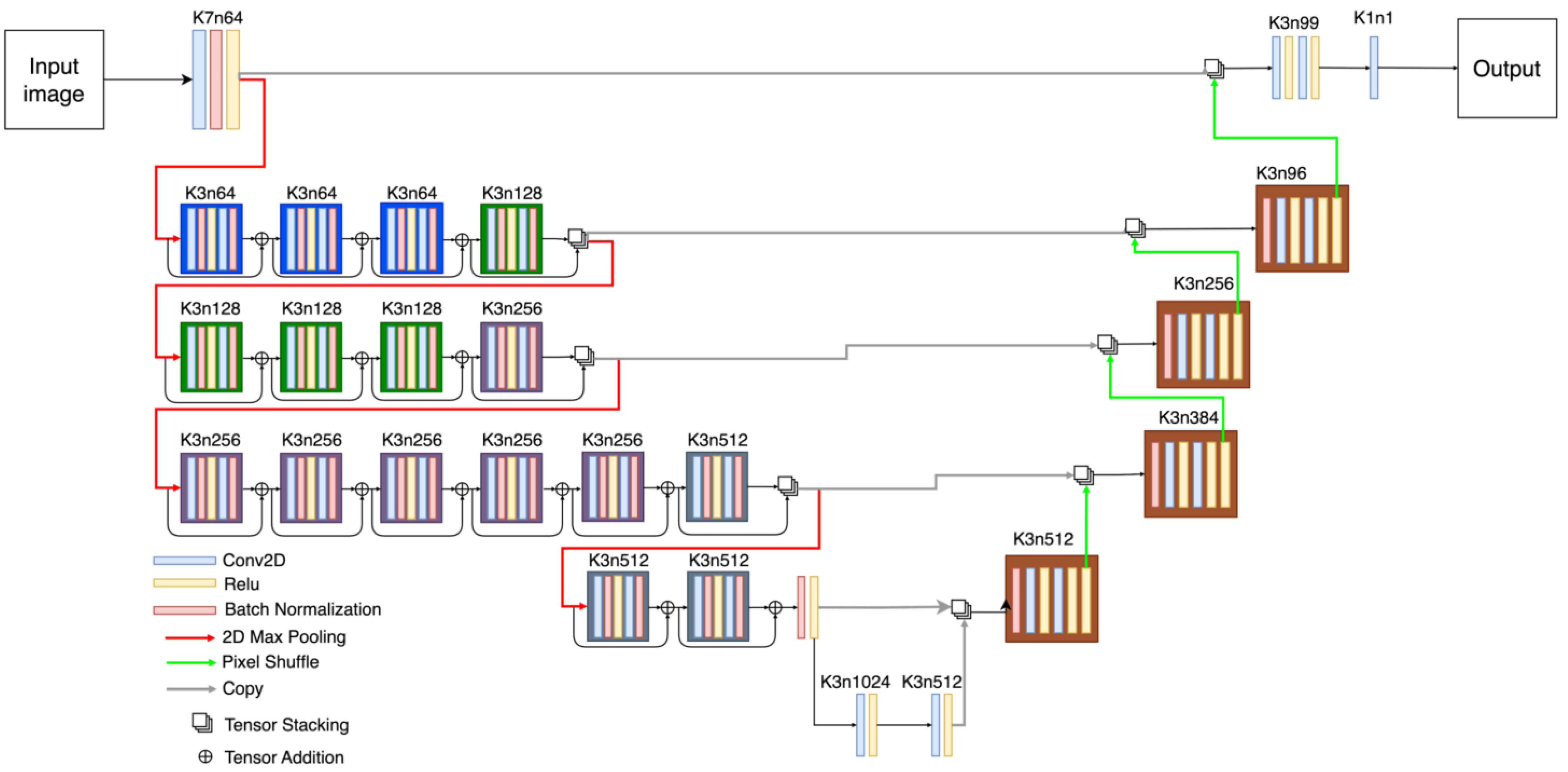
In terms of UNet-like architectures, the three selected UNets have quite diverse detailed structures as can be appreciated in Figure 2, Figure 3 and Figure 4. The DUNet uses dense connections between its layers. RUNet uses residual blocks in its layer, and AUNet uses bottleneck blocks with global block residual addition and residual cores. The following sections provide more insight into the network architecture.
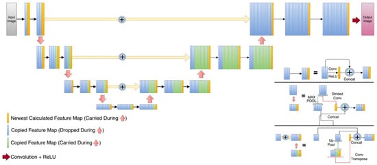
Figure 2.
Dense UNet (DUNet) architecture. Orange rectangles represent the newly calculated feature maps at every level. Blue rectangles are the feature maps that are dropped during the expansion path and green rectangles are the feature maps that are copied during the expansion path.

Figure 3.
Robust UNet (RUNet) architecture. The number that follows ‘k’ represents the size of the kernel and the number that follows ‘n’ represents the number of filters.
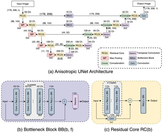
Figure 4.
(a) Anisotropic UNet (AUNet) Architecture, (b) Bottleneck Block, and (c) Residual Core.
2.3. Dense UNet (DUNet)
In the employed DUNet shown in Figure 2, the contraction path of this network [21], which was inspired by dense convolutional neural network layers [52], the input images are subjected to a convolutional layer and a max pool function for their representation in a lower dimension. A total of four downsampled layers were applied to a matrix of 22 × 26. The DUNet expansion path uses convolutional transpose layers to reconstruct the images at higher dimensionality. The latter was set to be 176 × 208, which is the dimensionality of the HQ images (which also serves as the ground truth).
2.4. Robust UNet (RUNet)
As illustrated in Figure 3, the RUNET architecture uses blocks with a combination of convolutions followed by batch normalization [53] and ReLU operation [54] followed by a tensor addition to so-called residual blocks (RB). The contraction path has four levels, and each level has multiple residual blocks, which are connected via skip connections; this creates a complex representation of the features at every level. Max pool operation is used to reduce the filter maps’ dimensionality; it uses convolutional 2D layers, followed by batch normalization, ReLU activation, and residual additions, allowing the network to learn complex representations of the input images. The expansion path uses a batch normalization layer at the input followed by a combination of convolution and ReLU activation layers. Feature maps are then pixel shuffled to change the dimension before combining the output of the previous contraction (Kth level) layer with the output of the expansion layer (K + 1 level) via tensor stacking, i.e., the tensors are stacked to form more feature channels. The last layer of the expansion path uses convolution with a kernel size of 1 to reconstruct the output image.
2.5. Anisotropic UNet (AUNet)
This network considers that the input images may not be isotropic (i.e., voxel size is not the same in all three dimensions) [23]. In our studies, we use isotropic 2D images, and so we implemented the AUNet architecture with only two-dimensional traits by replacing 3D operations with 2D operations. Figure 4 shows the AUNet, illustrating that it is based on two major components: the Bottleneck Block (BB), which simulates the isotropic down- and upsampling, and the Residual Core (RC), which makes it possible to have more convolutional layers at each level. In particular, the AUNet runs the 176 × 208 image through a combination of residual cores and a max-pooling layer; the resulting encoded image goes through the expansion path subjected to a deconvolution layer, a concatenation layer, and residual cores. The output from the top layers of the contraction layer is used as input to the BB before concatenating at the expansion path. We used a BB based on the one reported by Lin. et al. [23]. The BB shrinks half of the feature maps of the previous layer on consecutive 3 × 3 convolutional layers between two endpoint convolutions with a kernel size of 1 × 1. All convolution layers are activated by ReLU and Batch Normalization. To increase the convolution operation at every level, we design an RC inspired by Lin et al. [23] that takes a combination of 3 × 3 kernelled convolutional layers, followed by batch normalization layers. A skip connection is added that convolves the input with a 1 × 1 kernel and adds the features with the output of previous convolutional layers. The joined features go through a ReLU and Batch normalization layer to attain the residual core’s result.
2.6. Network Implementation and Training
All networks were created using Keras with TensorFlow 2.2. Training and testing were performed on the Sabine clusters at the University of Houston Hewlett Packard Enterprise Data Science Institute (HPE DSI) on Nvidia V100 tensor core GPUs, in all experiments, we used the Adam optimizer [55], with a mean squared error loss function, a learning rate of 0.001, and a batch size of 32. Each of the three UNets and each of the two acquisition scenarios (6 cases of training sessions) were trained for 100 and 1000 epochs. The best results were obtained when a constant learning rate was used to run all the epochs. Experiments with dynamic learning rates produced inferior results and are not part of this paper.
The learning rate parameter was chosen based on the common trait that the network uses dense and convolution layers and a learning rate of 0.001 has shown the best results when dense layers were chosen. A similar learning rate can be seen in the literature, as well [21,22,23]. We used mean squared error as our loss function for training all the neural networks. We recognize that the loss function will also have a great impact on the upscaling of the images; however, a detailed comparison of different loss functions, which may include mean squared errors, mean intensity errors, structural similarity, edge enhancement loss, and perceptual loss, to name a few, is beyond the scope of this paper, and will be explored in one of our future works. As can also be seen in the literature, the mean squared error is able to produce a pixel-by-pixel loss and can work satisfactorily for our problem [21,22,23] as it is commonly used to upscale images.
Since neural architectures typically use input images with the same digital matrix sizes, our datasets were pre-processed before being used as inputs to the networks. Specifically, our datasets included 176 × 208 augmMRI images and one of synLQ that was 22 × 26, 44 × 52, or 88 × 104. Preprocessing entailed interpolating the synLQ images to 176 × 208 using the nearest-neighbor interpolation to preserve the image distribution at high resolution, and the pixel values are normalized in the range of 0–1 to avoid gradient explosion [56,57]; subsequently, identically sized synLQ and augmMRI images were stacked together and supplied to the networks.
Training and validation loss was monitored to avoid overfitting of the networks. The difference between the training loss and validation loss indicates that there is no overfitting. To further ensure that there is no overfitting, only the best weight from the training process is taken, which corresponds to the lowest validation loss. To prevent bias from data leakage, training, and testing were performed on images collected from different subjects.
2.7. Data Analysis and Statistics
To assess the performance of the three UNets to upscale images, we used four standard metrics in comparing the reconstructed (reconHQ) to the corresponding ground truth: the pixel-wise Mean Squared Error (MSE), the pixel-wise Mean Intensity Error (MIE), the Mean Structural Similarity Index (SSIM) and the Peak Signal to Noise Ratio (PSNR). In this study, these four metrics formed the response variables. Data collection involves a repeated measure design applied to each of the test images. As image-to-image variation is inevitable, for the purpose of statistical analysis we employ mixed-effects (aka, repeated measure) modeling to account for the fact that the same images are used more than once. In the adequacy checking tests performed on each model, we observed that when we used the MSE and MIE as the response, the standard assumptions of mixed effects model were violated. To overcome this issue, we use the natural logarithm transformation on both MSE and MIE. In summary, the final response variables for the mixed effects modeling analysis were log(MSE), log(MIE), SSIM, and PSNR.
We had a total of four fixed variables for the mixed-effect models. These variables were: the type of Unet (DUNet, AUNet, and RUNet), input matrix size (1/8, 1/4, and 1/2), acquisition scenarios (With-Prior and WithOut-Prior), and the number of training epochs (100 and 1000). We observe substantial differences in summary statistics when we compare With-Prior and WithOut-Prior; therefore, we performed mixed effects modeling on them separately. In a sensitivity analysis, we found that the summary statistics from 100 epochs to 1000 epochs did not show a significant change in the actual values; hence, we performed MEM only on results obtained by training Unet models only for 100 epochs. Therefore, two fixed variables are employed in our MEM model, which are the type of Unet (DUNet, AUNet, and RUNet) and the input matrix size (1/8, 1/4, and 1/2). In addition to the above two fixed variables, we also consider their interaction in the mixed effects model.
Descriptive statistics were first calculated for each response variable (i.e., the evaluation metrics) for the different fixed effects (aka explanatory) variables, that is the three types of Unets and the three matrix sizes, as shown in Table 1, Table 2 and Table 3. Each response was tested using mixed effects modeling, with the fixed effects chosen as the explanatory variables, while the 540 test images constituted the random effects. The mixed effects model examined the significance of explanatory variables taking into account the significant image-to-image variation (i.e., incorporating the repeated measure aspect design that we have in this study, where multiple measurements are performed in each of the 540 test images).

Table 1.
Upscaling a 1/8 downsampled (22 × 26) synLQ with the three Unets. The best results are represented in bold. The numbers represent the mean value followed by the standard deviation in parenthesis.

Table 2.
Upscaling a 1/4 downsampled (44 × 52) synLQ with the three Unets. The best results are represented in bold. The numbers represent the mean value followed by the standard deviation in parenthesis.

Table 3.
Upscaling a 1/2 downsampled (88 × 104) synLQ with the three Unets. The best results are represented in bold. The numbers represent the mean value followed by the standard deviation in parenthesis.
3. Results
Figure 5 reports the validation and training losses for the three Unets and the two acquisition scenarios, illustrating that, in all six cases, these networks exhibit rather quick convergence. The training losses for all cases converge in the first couple of epochs (Figure 5a,b); however, a gradual reduction in loss can be seen for all three networks throughout the training, while the validation losses converge by the 20th epoch (Figure 5c,d), i.e., a plateau is reached and then the loss fluctuates, which is the desired observation. Specifically, the validation losses for the AUNet and RUNet converge by the 15th epoch for the With-Prior scenario and by the 20th epoch for the WithOut-Prior scenario. Notably, the DUNet validation loss converges within the first four epochs; this may be related to the use of dense convolutional layers that can carry the outputs of one convolutional layer to all the future layers allowing the network to learn more complex representations of the images [33,52].


Figure 5.
Representative results from the training sessions depicting the training (a,b) and the validation (c,d) losses (as log mean squared error versus epochs) for the two acquisition scenarios: With-Prior (a,c) and the WithOut-Prior (b,d) information. These examples correspond to the worst-case scenario of upscaling 1/8 downsampled synLQ images toward the corresponding 176 × 208 synHQ. The networks were trained for 100 and 1000 epochs; the first 100 epochs are presented here.
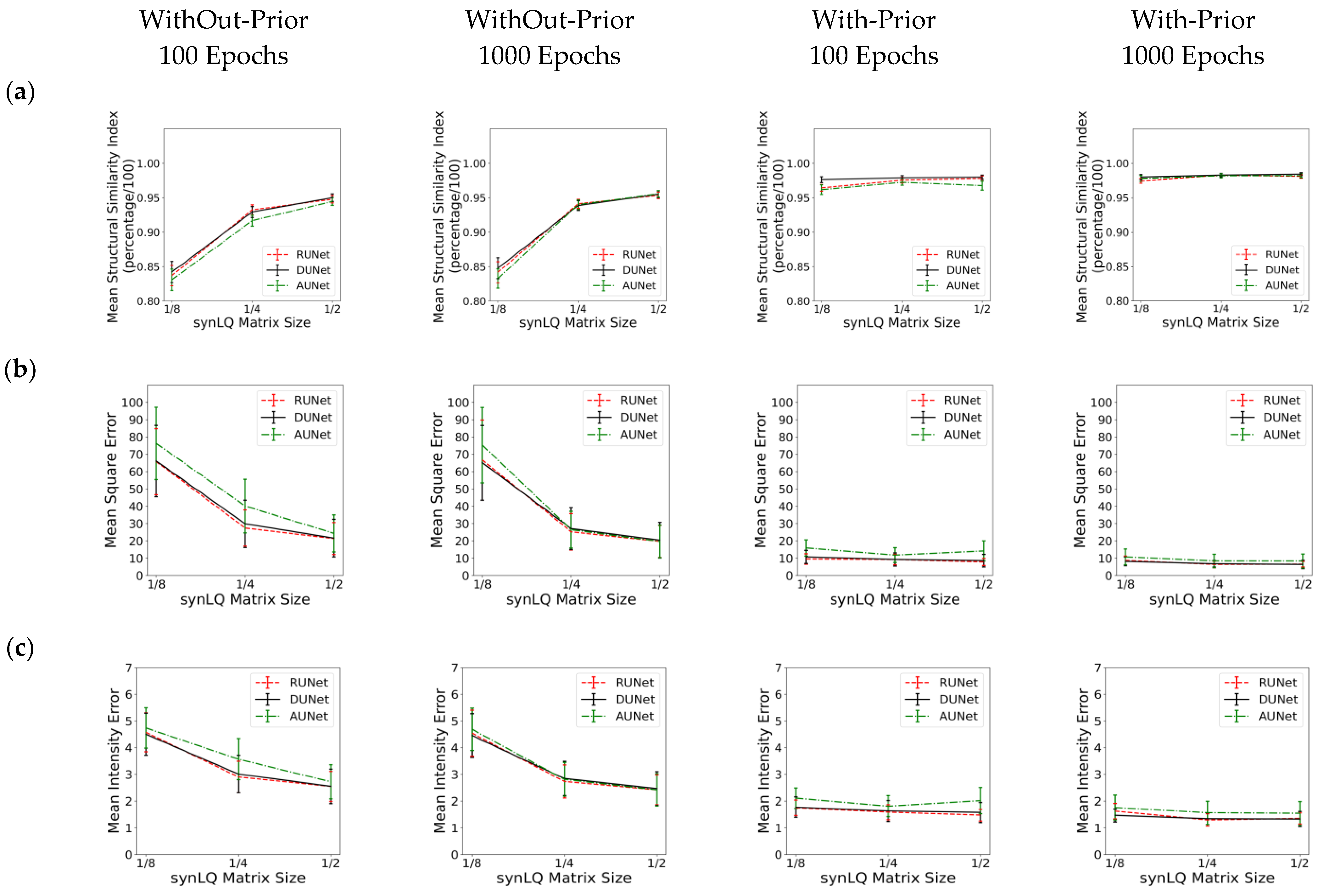
Table 1, Table 2 and Table 3 review the results from all studies corresponding to upscaling LQ-to-HQ images that were downsampled to 1/8, 1/4, and 1/2 of the complete matrix, respectively. Each table reports the results for the two scanning scenarios, and for 100 and 1000 epochs of training for each scenario. The first general observation is that, for the same scanning scenario and the same downsampled matrix, as observed by the values of the descriptive statistics, the three UNets exhibit somewhat similar performances, as reflected by the mean MSE, MIE, SSI, and PSNR values. This is an intriguing observation, indicating that all three choices of UNet perform similarly when sufficient training is performed. Figure 6 also shows that, for the same scanning scenarios, and the same downsampled image, there is virtually no difference between training for 100 or 1000 epochs.
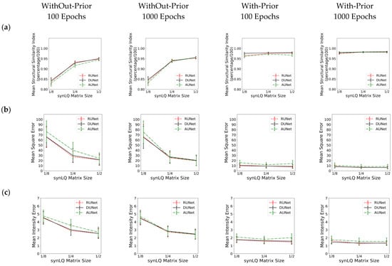

Figure 6.
Performance of the three UNet architectures (RUNet in red, DUNet in black, and AUNet in Green) for the two With- and WithOut-Prior acquisition scenarios after training for 100 and 1000 epochs. (a) Mean Structural Similarity Index, (b) Mean Squared Error, (c) Mean Intensity Error, and (d) Peak Signal-to-Noise Ratio of reconHQ vs. synHQ, for different sizes of input synLQ images. The measures are reported as average (standard deviation) for N = 540 test images corresponding to 84 subjects.
Substantial differences in performance of the UNets, however, are observed when comparing the two acquisition scenarios, as can be clearly seen in Table 1, Table 2 and Table 3, and in Figure 6. As compared to the cases of With-Prior, upscaling of downsampled LQ images with the WithOut-Prior scenario exhibit lower SSIM, higher MSE, higher MIE, and lower PSNR, i.e., the performance of the UNet WithOut-Prior is worse than that of With-Prior. In the With-Prior cases, the physically collected (and augmented) augmMRI provide additional anatomical and morphological data about the same structures in the object, resulting in upscaling being closer to the ground truth synHQ (i.e., complete matrix with reduced noise), as also reported in [21]. The LQ images at the WithOut-Prior scenario can also be upscaled to a different degree, depending on the size of the synLQ. Indeed, when the cases of WithOut-Prior are considered (the graphs in the two leftmost columns), the UNets upscale 1/8 downsampled images with lower accuracy. This result reflects the fact that at lower resolution (larger voxel size) finer structural details may be lost. Such finer structures; however, may be recoverable by the UNet in With-Prior scenario in the case that they are preserved in the augmMRI image.
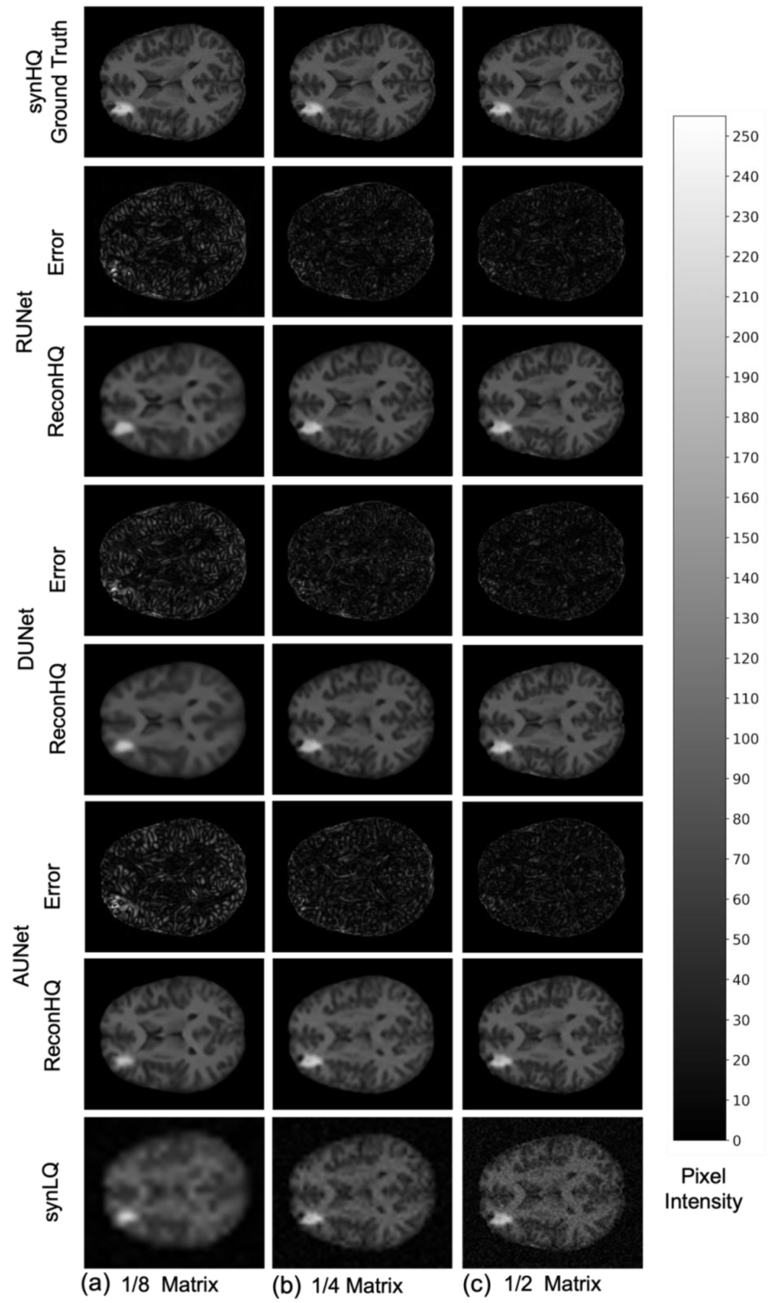
The performance of the UNets may also be appreciated in Figure 7 and Figure 8, which show the reconHQ images together with pixel-by-pixel differences with respect to the ground truth (i.e., |reconHQ—synHQ|) for the three networks at different synLQ sizes and two scanning scenarios. It can be observed that lesion reconstruction is better in the With-Prior compared to WithOut-Prior acquisition scenario for the 1/8 downsampled synLQ.
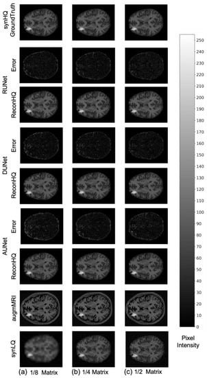
Figure 7.
Representative example of reconstructed images and errors versus ground truth with the three UNets trained for 100 epochs with the With-Prior acquisition scenario (i.e., including the augmMRI) to upscale (a) 1/8 downsampled (22 × 26) and (b) 1/4 downsampled (44 × 52) and (c) 1/2 downsampled (88 × 104) synLQ. The Error intensity in this figure is five times the original intensity.

Figure 8.
Representative example of reconstructed images and errors versus ground truth with the three UNets trained for 100 epochs with the WithOut-Prior acquisition scenario (i.e., not including the augmMRI) to upscale (a) 1/8 downsampled (22 × 26) and (b) 1/4 downsampled (44 × 52) and (c) 1/2 downsampled (88 × 104) synLQ. The error intensity in this figure is three times the original intensity.
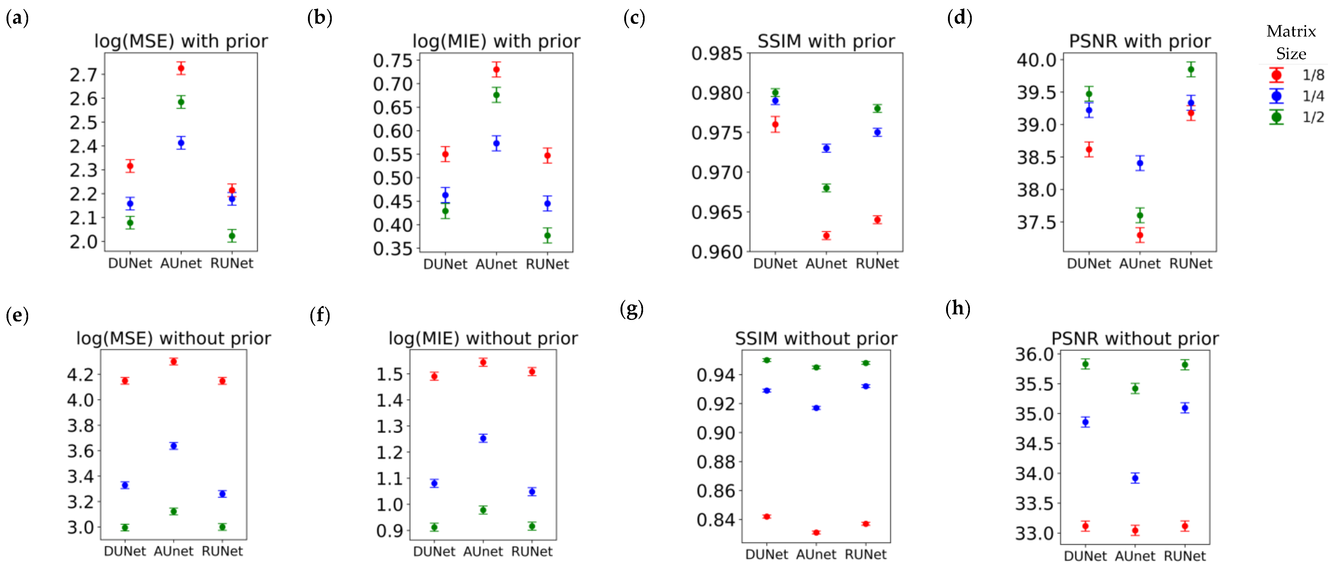
Table 4 shows the results for the F-ratio obtained for fixed effects in the MEM. The F-ratio corresponds to the F-test performed in the mixed-effect model that was fitted each time. For more information one can refer to [43]. In the freeware R, which was used to fit the models, F-test values can be derived using the anova(.) option for a fitted model lmer(.) from the library lme4. We test the significance of type of UNet, matrix size and the interaction of the type of UNet and the matrix size. We provide the F-ratios for each of the terms that were used in each mixed effect model. The observed F-ratios are very large, and as a result, all of their respective p-values were well below 0.01 (the level of significance alpha), which means that the type of UNet, the input matrix size, and their interaction are all highly statistically significant factors. Therefore, we only present F-ratios and not the p-values in the table, as the latter in all cases would have been identical, i.e., << 0.01. The actual interaction plot between the fixed variables can be observed in Figure 9 for With-Prior and WithOut-Prior acquisition scenario, indicating the relative performance for every response metric for all possible combination of the two factors that we examine in our mixed effect model.

Table 4.
F-ratios showing the significance of each of the terms that were used in the mixed effects model. Each term is highly statistically significant as all the F-ratios are large, resulting for all cases in p-values << 0.01.
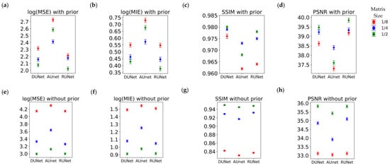
Figure 9.
Interaction plots for the mixed-effects model, indicating how the two factors—UNets and Matrix Size—interact with each other under (a–d) the With-Prior acquisition scenario (a) log(MSE), (b) log(MIE), (c) SSIM, and (d) PSNR; and under (e–h) the WithOut-Prior acquisition scenario (e) log(MSE), (f) log(MIE), (g) SSIM, and (h) PSNR.
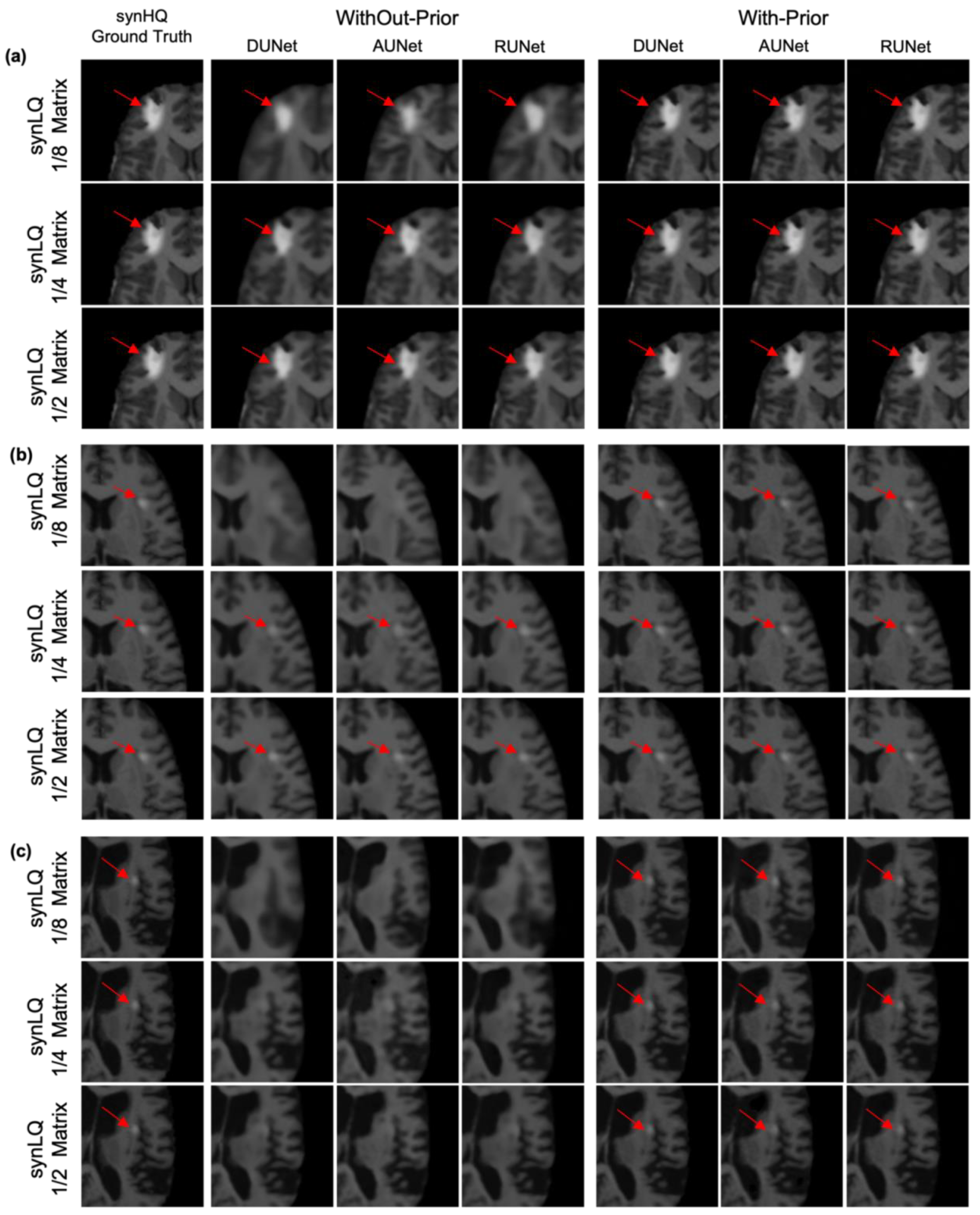
Inspection of WithOut-Prior data sets that resulted in reconstructions that exhibited lower scores (SSIM less than 83% for 1/8 matrix and less than 91% for 1/4 matrix) pointed to the anticipated effect of lesion size and contrast relative to the neighboring tissue, representative examples of which are shown in Figure 10. Figure 10a shows a case where the lesion is rather large (greater than 8 pixels in a single dimension) and the intensity of the lesion is significantly higher than neighboring pixel values (greater than 100 on a 0–255 scale). Figure 10b corresponds to cases that the lesion (i) is not observed in the upscaled images (reconHQ) that were reconstructed from the 1/8 downsampled synLQ images for the WithOut-Prior acquisition scenario, and (ii) is observable (arrow) in the reconstructed images for the larger downsampled matrices for all three UNets in the two acquisition scenarios. These cases correspond to lesions that were eight (8) or fewer pixels in size in any dimension, and whose signal intensity was high with respect to neighboring pixels (greater than 50 on a scale of 0–255). When an image is downsampled to 1/8, then a lesion 8 pixels in length would correspond to a single pixel of the downsampled image. In the Without-Prior case, the low-signal-intensity lesion cannot be recovered; however, with HQCP, this is feasible. Figure 10c depicts another case in which the lesion is not observable without HQCP (columns 2–4); however, the lesion becomes visible when HQCP are available (columns 5–7). This case is representative of all lesion information lost when (i) the contrast difference between the lesion and neighboring pixel is low (less than 30 on a 0–255 scale), and (ii) the lesion is small in size (fewer than 8 pixels in a single dimension).
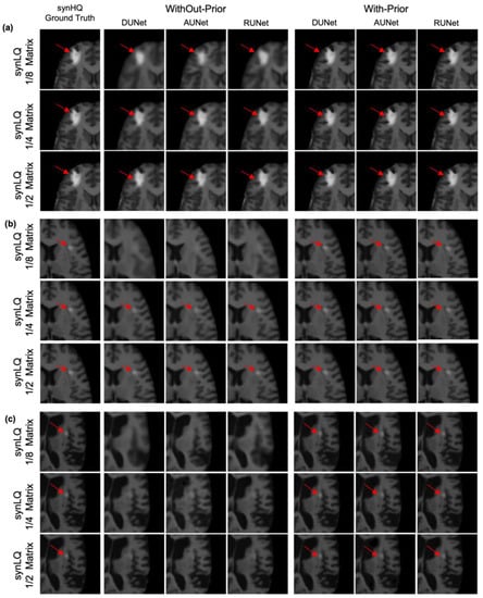
Figure 10.
Characteristic examples of upscaling a 1/8 downsampled (22 × 26), a 1/4 downsampled (44 × 52) and a 1/2 downsampled (88 × 104) synLQ image, of the same set) toward the synHQ ground truth. The figure shows a comparison of two acquisition scenarios: With-Prior and WithOut-Prior. (a) Scenario where the tumor is visible in all reconstruction scenarios; (b) where the tumor is not visible during reconstruction of 1/8 downsampled synLQ cases in the WithOut-Prior acquisition scenario; (c) where the tumor is barely visible during reconstruction of almost all the synLQ cases in the WithOut-Prior acquisition scenario. This figure shows that it is impossible to reconstruct a tumor if the tumor is not visible in the synLQ images in the WithOut-Prior acquisition scenario.
4. Discussion
The ability of UNets to create an image-to-image translation makes them a suitable neural network model for improving low quality MR images post acquisition. As demonstrated herein and in prior works [21,22,23,24,25,26,27], UNets can be designed and then trained to seek features between pairs of LQ and HQ MRI of the same exact view of the same object; the trained UNet can then be used to upscale a new LQ to its (unknown) HQ image. This performance may relate to the endogenous capability of UNet architectures to identify anatomical and/or morphological features [21,22,23,24,25,26,27,28,33,34,35], which are the basis for accurately describing a pixel-by-pixel transformation between the downsampled noisy LQ image and the complete matrix HQ one. Moreover, in this work, since the UNets were trained with noiseless ground truths, i.e., the synthesized synHQ images, the reconstructed upscaled images were noiseless. This denoising action is a direct highlight of the fact that the features and quality of the reconstructed images depends on the corresponding features and quality of ground truths.
The tested UNets indicated several common characteristics. First, all three UNets exhibited similar performance manifested by summary statistics when trained and tested for the same data sets, for the same downsampled original images (the synLQ images) and the same acquisition scenario. This was a rather unexpected outcome; it suggests that the UNet architecture might be a robust backbone for revealing structural image features, irrespective of the variations in the architecture of the individual networks. Another observation is that all three UNets converged within the 25th epoch (Figure 5). This is also evident from Table 1, Table 2 and Table 3, which report performance of the three UNets after 100 and 1000 epochs: there is no significant improvement in any of the four evaluation metrics. For example, the training losses at 100 and 1000 epochs differ by 0.0002/1.0, while the validation losses are less than 0.0001/1.0. The primary difference between them was that DUNet training and validation losses indicated convergence within the first couple of epochs. The origin of this rather rapid convergence was not identified.
The outcomes of these studies further emphasize that the effectiveness of upscaling with the studied UNets depends on the actual image acquisition parameters, such as: (i) the matrix size of the downsampled image; (ii) the structure(s) of interest, including their size relative to the spatial resolution of the downsampled image, and their contrast relative to the surrounding matter; and (iii) whether a complementary image was available (or in an actual study, was acquired and included in the network training). As reflected in Table 1, Table 2 and Table 3, the synLQ matrix size affected upscaling and, as expected, the worst performance corresponded to upscaling the 1/8 downsampled images. Based on the structural similarity indexes, UNet-upscaled 1/2, and 1/4 downsampled images exhibited up to 95% ± 0.50% and 93.24% ± 0.73% similarity, respectively, with respect to the ground truth in the worst-case scenario of WithOut-Prior. In contrast, the 1/8 downsampled images, when upscaled with the WithOut-Prior acquisition scenario, had a similarity of 84% ± 1.5% to the ground truth. Notably, when complementary priors were used, the UNet upscaled 1/8 downsampled had a 97% ± 0.40% similarity to the ground truth. While the reported metrics offer a useful quantitative performance of the upscaling, as statistical entities calculated over the entire image, these metrics do not provide information about the success of upscaling details of structures. Indeed, inspecting data sets with low similarity indices, it became apparent that the UNets were not accurately reproducing the margins of lesions or edges of white and gray matter (Figure 8a–c).
What is well known from experimental and clinical imaging also appears to be reflected in the outcome of this study: if contrast and resolution are insufficient, a structure of interest will not be captured and “resolved/revealed” in the upscaling. This is the case when considering the upscaling of 1/8 downsized images in the acquisition scenario without complementary information: lesions with low contrast relative to their surrounding tissue are not recoverable. While this is an expected finding as a result of the basic imaging physics, this can also be considered to be a manifestation of the natural limit of UNets.
However, as also seen in Figure 10c, the same lesion that could not be recovered in the single image acquisition scenario could be clearly recognized when the complementary image was included. Obviously, this occurs because the complementary image carries the needed structural information: when combined with perfect spatial matching, the UNet training ensures that information is used in the upscaling of the LQ images. However, there are acquisition scenarios in which a HQCP image cannot be collected, as in the cases of different main magnetic field systems, or motion regimes that do not allow matching of an LQ and an HQCP image set. These findings warrant additional systematic studies of these effects on a wider range of data to better establish the practical role of deep learning-based upscaling with clinical utility; we plan to explore these in future research. We may then envision that the design and use of future imaging protocols to entail processes that integrate the selection of acquisition parameters (e.g., acquisition matrix and number of repetitions) based on how these affect the performance of a deep learning technique in upscaling the images (e.g., improve resolution, SNR or CNR).
The statistical analysis using the mixed-effect model showed that the interaction of UNet architecture and the size of the acquisition matrix were highly statistically significant as seen in Table 4, and Figure 9 and illustrated that bottleneck layers (AUNet) performed suboptimally, and in cases of small lesions, they were not recovered. Upscaling in the WithOut-Prior scenario is inferior to that in the With-Prior scenario, a behavior that was exemplified in the more undersampled LQ. Lesions with sizes smaller than eight pixels and with low contrast were not recovered in the WithOut-Prior scenario, specifically in the case of 1/8 undersampling.
This study has certain limitations. First, a rather small sample of original images was used (436 images from the OASIS dataset with each image corresponding to a different subject), and we added synthetic hyperintense and homogeneous lesions. We augmented the training and testing dataset by additional image synthesis to increase variability, based on accepted practices [21,33,35]. Second, the current work is focused on comparing on three stat-of-the-art UNet models. While UNets appear robust and effective for the investigated datasets, in the light of rapid evolution of DL methodology, more networks should be investigated.
Future works will systematically assess the effect of the size and variability of the datasets in the accuracy of training. This may be done by combining multiple available data sets, incorporating additional alterations of morphology and anatomy secondary to pathologies, including same-subject multislice or 3D data sets, the presence of image artifacts, and even multi-contrast complementary priors. In future studies, we also plan to compare and investigate the effect of using bicubic [15] or nearest neighbor interpolations for preprocessing LQ images to the ground truth before being passed to the network and will also compare using an upscaling block as part of the network [58] which takes the LQ image as inputs in its low matrix sizes, without being preprocessed with any interpolation method. The main focus of the current study was on comparing three state-of-the-art UNet architectures for upscaling LQ MRI. In future work, we aim to perform additional experiments and comparison with super-resolution techniques and will provide more extensive comparison of model performance, model parameters, and the overall quality of upscaled images with other networks like generative models [30,31,32,59], CNN [16,60], and visual transformers [61,62,63], as well as comparing the impact of different training structures (supervised, unsupervised, and semi-supervised), rather than the actual layers of the model.
In addition to the above, we currently use publicly available MRI datasets and have not added experimental data from a new set of cohorts. This does not affect the study, as this work does not introduce any new neural network architecture. Rather, in this in silico work, we tested whether three neural architectures that are significantly different from each other were able to upscale images with significant difference. Our experiments support the conclusion that a different neural network can upscale images that visually appear similar to each other regardless of the actual layers of the architecture. This study supports the notion that attention must be paid to how the actual data are collected.
All three UNets upscaled LQ MRI to a different degree, indicating that one must be cautious of how ML is applied, interpreted, and used practically. In the With-Prior scenario, LQ images can be reliably upscaled; this contributes to the tradeoff between acquisition time and image quality of X-nuclei or spectroscopic imaging. In the WithOut-Prior case, since small and low contrast lesions may be lost, we may need to consider new approaches that entail the concurrent customization of deep learning and acquisition protocols. Overall, the results reflect what is expected from MR physics and known to the community: in single-contrast images, if a structure is not there you cannot recover it, unless you have some complementary contrast information. The critical aspect is what data are available: resolution, contrast SNR and especially the presence or not of same subject complementary information.
This pilot study further supports the notion that, in certain cases, the particular layers and architecture of UNet may not be important. Effort may, rather, focus on alternative metrics of desired image features such as cost functions, hyperparameters and training protocols in machine learning. Furthermore, the results point to the incorporation of the most obvious and ultimate, in our opinion, criterion in ML pipeline and application: the end-user, i.e., radiologists or other specialists, to ensure and access the merit of such techniques in the clinical realm.
5. Conclusions
The appropriate statistical analysis, MEM, for the problem under study (repeated measurement on test images) identified high statistical significance for the contribution of type of UNet, matrix size and their interaction for all four response variables (i.e., evaluation metrics) considered. In contrast, visual, subjective, impressions of the UNet reconstructed images demonstrate no clear difference in performance among them. These observations suggest that the detailed architecture and layers used in these particular UNets may not play a critical role in performance. In regard to the two acquisition scenarios, and as expected, the presence of same-subject complementary priors substantially improves the effectiveness of upscaling with any of the tested UNet where, again, there was no visual inspection difference in performance. Moreover, the study pointed to the fact that the size and the contrast of LQ images play an important role in the upscaling problem, especially when complementary information is not available. The outcomes support the notion that ML methods may have merit as an integral part of integrated holistic approaches in advancing MRI acquisitions; however primary attention should be paid to the foundational step of such approaches, i.e., the actual data collected.
Author Contributions
Conceptualization, R.S., P.T., A.G.W. and N.V.T.; methodology, R.S., P.T. and N.V.T.; Software R.S. and P.T.; Validation, R.S., P.T. and N.V.T.; formal analysis, R.S., P.T., A.G.W., I.S., C.L., E.L. and N.V.T.; investigation, R.S., P.T., A.G.W., I.S., C.L., E.L. and N.V.T.; resources, P.T. and N.V.T.; data curation, R.S. and P.T.; writing—original draft preparation, R.S., P.T. and N.V.T.; writing—review and editing, R.S., P.T., A.G.W., I.S., C.L., E.L. and N.V.T.; visualization, R.S., P.T. and N.V.T.; supervision, N.V.T.; project administration, N.V.T.; funding acquisition, N.V.T. All authors have read and agreed to the published version of the manuscript.
Funding
This work was supported in part by the National Science Foundation grant number CNS-1646566.
Institutional Review Board Statement
Not applicable.
Informed Consent Statement
Not applicable.
Data Availability Statement
The data presented in this study are openly available in OASIS-1 repository, reference number [49].
Acknowledgments
The authors acknowledge the use of the Sabine Cluster and the advanced support from the Research Computing Data Core at the University of Houston to carry out the research presented here.
Conflicts of Interest
The authors declare no conflict of interest.
References
- Parker, D.L.; Gullberg, G.T. Signal-to-Noise Efficiency in Magnetic Resonance Imaging. Med. Phys. 1990, 17, 250–257. [Google Scholar] [CrossRef] [PubMed]
- Constable, R.T.; Henkelman, R.M. Contrast, Resolution, and Detectability in MR Imaging. J. Comput. Assist. Tomogr. 1991, 15, 297–303. [Google Scholar] [CrossRef] [PubMed]
- Macovski, A. Noise in MRI. Magn. Reson. Med. 1996, 36, 494–497. [Google Scholar] [CrossRef] [PubMed]
- Plenge, E.; Poot, D.H.J.; Bernsen, M.; Kotek, G.; Houston, G.; Wielopolski, P.; van der Weerd, L.; Niessen, W.J.; Meijering, E. Super-Resolution Methods in MRI: Can They Improve the Trade-off between Resolution, Signal-to-Noise Ratio, and Acquisition Time? Magn. Reson. Med. 2012, 68, 1983–1993. [Google Scholar] [CrossRef]
- Peters, D.C.; Korosec, F.R.; Grist, T.M.; Block, W.F.; Holden, J.E.; Vigen, K.K.; Mistretta, C.A. Undersampled Projection Reconstruction Applied to MR Angiography. Magn. Reson. Med. 2000, 43, 91–101. [Google Scholar] [CrossRef]
- Lustig, M.; Donoho, D.; Pauly, J.M. Sparse MRI: The Application of Compressed Sensing for Rapid MR Imaging. Magn. Reson. Med. 2007, 58, 1182–1195. [Google Scholar] [CrossRef]
- Heidemann, R.M.; Özsarlak, Ö.; Parizel, P.M.; Michiels, J.; Kiefer, B.; Jellus, V.; Müller, M.; Breuer, F.; Blaimer, M.; Griswold, M.A.; et al. A Brief Review of Parallel Magnetic Resonance Imaging. Eur. Radiol. 2003, 13, 2323–2337. [Google Scholar] [CrossRef]
- Pruessmann, K.P. Encoding and Reconstruction in Parallel MRI. NMR Biomed. 2006, 19, 288–299. [Google Scholar] [CrossRef]
- Brateman, L. Chemical Shift Imaging: A Review. Am. J. Roentgenol. 1986, 146, 971–980. [Google Scholar] [CrossRef]
- Marques, J.P.; Simonis, F.F.J.; Webb, A.G. Low-field MRI: An MR Physics Perspective. J. Magn. Reson. Imaging 2019, 49, 1528–1542. [Google Scholar] [CrossRef]
- Hu, R.; Kleimaier, D.; Malzacher, M.; Hoesl, M.A.U.; Paschke, N.K.; Schad, L.R. X-nuclei Imaging: Current State, Technical Challenges, and Future Directions. J. Magn. Reson. Imaging 2020, 51, 355–376. [Google Scholar] [CrossRef] [PubMed]
- Pham, C.-H.; Ducournau, A.; Fablet, R.; Rousseau, F. Brain MRI Super-Resolution Using Deep 3D Convolutional Networks. In Proceedings of the 2017 IEEE 14th International Symposium on Biomedical Imaging (ISBI 2017), Melbourne, Australia, 18–21 April 2017; pp. 197–200. [Google Scholar]
- Chen, Y.; Shi, F.; Christodoulou, A.G.; Xie, Y.; Zhou, Z.; Li, D. Efficient and accurate MRI super-resolution using a generative adversarial network and 3D multi-level densely connected network. In Lecture Notes in Computer Science (Including Subseries Lecture Notes in Artificial Intelligence and Lecture Notes in Bioinformatics); LNCS; Springer: Cham, Switzerland, 2018; Volume 11070. [Google Scholar]
- van Reeth, E.; Tham, I.W.K.; Tan, C.H.; Poh, C.L. Super-Resolution in Magnetic Resonance Imaging: A Review. Concepts Magn. Reson. Part A 2012, 40A, 306–325. [Google Scholar] [CrossRef]
- Cherukuri, V.; Guo, T.; Schiff, S.J.; Monga, V. Deep MR Brain Image Super-Resolution Using Spatio-Structural Priors. IEEE Trans. Image Process. 2020, 29, 1368–1383. [Google Scholar] [CrossRef] [PubMed]
- Li, Y.; Iwamoto, Y.; Lin, L.; Xu, R.; Tong, R.; Chen, Y.-W. VolumeNet: A Lightweight Parallel Network for Super-Resolution of MR and CT Volumetric Data. IEEE Trans. Image Process. 2021, 30, 4840–4854. [Google Scholar] [CrossRef] [PubMed]
- Chen, F.; Taviani, V.; Malkiel, I.; Cheng, J.Y.; Tamir, J.I.; Shaikh, J.; Chang, S.T.; Hardy, C.J.; Pauly, J.M.; Vasanawala, S.S. Variable-Density Single-Shot Fast Spin-Echo MRI with Deep Learning Reconstruction by Using Variational Networks. Radiology 2018, 289, 366–373. [Google Scholar] [CrossRef]
- Pizurica, A.; Wink, A.; Vansteenkiste, E.; Philips, W.; Roerdink, B.J. A Review of Wavelet Denoising in MRI and Ultrasound Brain Imaging. Curr. Med. Imaging Rev. 2006, 2, 247–260. [Google Scholar] [CrossRef]
- Zhang, K.; Zuo, W.; Chen, Y.; Meng, D.; Zhang, L. Beyond a Gaussian Denoiser: Residual Learning of Deep CNN for Image Denoising. IEEE Trans. Image Process. 2017, 26, 3142–3155. [Google Scholar] [CrossRef]
- Fan, L.; Zhang, F.; Fan, H.; Zhang, C. Brief Review of Image Denoising Techniques. Vis. Comput. Ind. Biomed. Art 2019, 2, 7. [Google Scholar] [CrossRef]
- Iqbal, Z.; Nguyen, D.; Hangel, G.; Motyka, S.; Bogner, W.; Jiang, S. Super-Resolution 1H Magnetic Resonance Spectroscopic Imaging Utilizing Deep Learning. Front. Oncol. 2019, 9, 1010. [Google Scholar] [CrossRef]
- Hu, X.; Naiel, M.A.; Wong, A.; Lamm, M.; Fieguth, P. RUNet: A Robust UNet Architecture for Image Super-Resolution. In Proceedings of the 2019 IEEE/CVF Conference on Computer Vision and Pattern Recognition Workshops (CVPRW), Long Beach, CA, USA, 16–17 June 2019. [Google Scholar]
- Lin, H.; Figini, M.; Tanno, R.; Blumberg, S.B.; Kaden, E.; Ogbole, G.; Brown, B.J.; D’Arco, F.; Carmichael, D.W.; Lagunju, I.; et al. Deep learning for low-field to high-field mr: Image quality transfer with probabilistic decimation simulator. In International Workshop on Machine Learning for Medical Image Reconstruction; Springer: Cham, Switzerland, 2019; pp. 58–70. [Google Scholar]
- Masutani, E.M.; Bahrami, N.; Hsiao, A. Deep Learning Single-Frame and Multiframe Super-Resolution for Cardiac MRI. Radiology 2020, 295, 552–561. [Google Scholar] [CrossRef]
- Chatterjee, S.; Sarasaen, C.; Rose, G.; Nürnberger, A.; Speck, O. DDoS-UNet: Incorporating Temporal Information Using Dynamic Dual-Channel UNet for Enhancing Super-Resolution of Dynamic MRI. arXiv 2022, arXiv:2202.05355. [Google Scholar]
- Chatterjee, S.; Sciarra, A.; Dunnwald, M.; Mushunuri, R.V.; Podishetti, R.; Rao, R.N.; Gopinath, G.D.; Oeltze-Jafra, S.; Speck, O.; Nurnberger, A. ShuffleUNet: Super Resolution of Diffusion-Weighted MRIs Using Deep Learning. In Proceedings of the 2021 29th European Signal Processing Conference (EUSIPCO), Dublin, Ireland, 23–27 August 2021; pp. 940–944. [Google Scholar]
- Ding, P.L.K.; Li, Z.; Zhou, Y.; Li, B. Deep Residual Dense U-Net for Resolution Enhancement in Accelerated MRI Acquisition. In Proceedings of the Medical Imaging 2019: Image Processing, San Diego, California, USA, 19–21 February 2019; p. 14. [Google Scholar]
- Nasrin, S.; Alom, M.Z.; Burada, R.; Taha, T.M.; Asari, V.K. Medical Image Denoising with Recurrent Residual U-Net (R2U-Net) Base Auto-Encoder. In Proceedings of the 2019 IEEE National Aerospace and Electronics Conference (NAECON), Dayton, OH, USA, 15–19 July 2019; pp. 345–350. [Google Scholar]
- Koonjoo, N.; Zhu, B.; Bagnall, G.C.; Bhutto, D.; Rosen, M.S. Boosting the Signal-to-Noise of Low-Field MRI with Deep Learning Image Reconstruction. Sci Rep. 2021, 11, 8248. [Google Scholar] [CrossRef] [PubMed]
- Mahapatra, D.; Bozorgtabar, B.; Garnavi, R. Image Super-Resolution Using Progressive Generative Adversarial Networks for Medical Image Analysis. Comput. Med. Imaging Graph. 2019, 71, 30–39. [Google Scholar] [CrossRef] [PubMed]
- Sanchez, I.; Vilaplana, V. Brain MRI Super-Resolution Using 3D Generative Adversarial Networks. arXiv 2018, arXiv:1812.11440. [Google Scholar]
- Lyu, Q.; Shan, H.; Wang, G. MRI Super-Resolution With Ensemble Learning and Complementary Priors. IEEE Trans. Comput. Imaging 2020, 6, 615–624. [Google Scholar] [CrossRef]
- Ronneberger, O.; Fischer, P.; Brox, T. U-Net: Convolutional networks for biomedical image segmentation. In International Conference on Medical Image Computing and Computer-Assisted Intervention; Springer: Cham, Switzerland, 2015; pp. 234–241. [Google Scholar]
- Çiçek, Ö.; Abdulkadir, A.; Lienkamp, S.S.; Brox, T.; Ronneberger, O. 3D U-Net: Learning dense volumetric segmentation from sparse annotation. In Proceedings of the International Conference on Medical Image Computing and Computer-Assisted Intervention—MICCAI 2016, Athens, Greece, 17–21 October 2016; Springer: Cham, Switzerland, 2016; pp. 424–432. [Google Scholar]
- Sharma, R.; Eick, C.F.; Tsekos, N.V. Myocardial Infarction Segmentation in Late Gadolinium Enhanced MRI Images Using Data Augmentation and Chaining Multiple U-Net. In Proceedings of the 2020 IEEE 20th International Conference on Bioinformatics and Bioengineering (BIBE), Cincinnati, Ohio, USA, 26–28 October 2020; pp. 975–980. [Google Scholar]
- Soomro, T.A.; Afifi, A.J.; Gao, J.; Hellwich, O.; Paul, M.; Zheng, L. Strided U-Net Model: Retinal Vessels Segmentation Using Dice Loss. In Proceedings of the 2018 Digital Image Computing: Techniques and Applications (DICTA), Canberra, Australia, 10–13 December 2018; pp. 1–8. [Google Scholar]
- Chen, C.; Zhou, K.; Wang, Z.; Xiao, R. Generative Consistency for Semi-Supervised Cerebrovascular Segmentation from TOF-MRA. IEEE Trans. Med. Imaging 2022, 1. [Google Scholar] [CrossRef]
- Chen, C.; Zhou, K.; Zha, M.; Qu, X.; Guo, X.; Chen, H.; Wang, Z.; Xiao, R. An Effective Deep Neural Network for Lung Lesions Segmentation from COVID-19 CT Images. IEEE Trans. Industr Inform. 2021, 17, 6528–6538. [Google Scholar] [CrossRef]
- Steeden, J.A.; Quail, M.; Gotschy, A.; Mortensen, K.H.; Hauptmann, A.; Arridge, S.; Jones, R.; Muthurangu, V. Rapid Whole-Heart CMR with Single Volume Super-Resolution. J. Cardiovasc. Magn. Reson. 2020, 22, 56. [Google Scholar] [CrossRef]
- Isensee, F.; Kickingereder, P.; Wick, W.; Bendszus, M.; Maier-Hein, K.H. No New-Net. In Brainlesion: Glioma, Multiple Sclerosis, Stroke and Traumatic Brain Injuries; Crimi, A., Bakas, S., Kuijf, H., Keyvan, F., Reyes, M., van Walsum, T., Eds.; Springer International Publishing: Cham, Switzerland, 2019; pp. 234–244. [Google Scholar]
- Zaaraoui, W.; Konstandin, S.; Audoin, B.; Nagel, A.M.; Rico, A.; Malikova, I.; Soulier, E.; Viout, P.; Confort-Gouny, S.; Cozzone, P.J.; et al. Distribution of Brain Sodium Accumulation Correlates with Disability in Multiple Sclerosis: A Cross-Sectional 23Na MR Imaging Study. Radiology 2012, 264, 859–867. [Google Scholar] [CrossRef]
- O’Reilly, T.; Webb, A.G. In Vivo T1 and T2 Relaxation Time Maps of Brain Tissue, Skeletal Muscle, and Lipid Measured in Healthy Volunteers at 50 MT. Magn. Reson. Med. 2022, 87, 884–895. [Google Scholar] [CrossRef]
- Pinheiro, J.C.; Bates, D.M. Mixed-Effects Models in S and S-PLUS; Springer: New York, NY, USA, 2000; ISBN 0-387-98957-9. [Google Scholar]
- Chlap, P.; Min, H.; Vandenberg, N.; Dowling, J.; Holloway, L.; Haworth, A. A Review of Medical Image Data Augmentation Techniques for Deep Learning Applications. J. Med. Imaging Radiat. Oncol. 2021, 65, 545–563. [Google Scholar] [CrossRef] [PubMed]
- Shin, H.-C.; Tenenholtz, N.A.; Rogers, J.K.; Schwarz, C.G.; Senjem, M.L.; Gunter, J.L.; Andriole, K.P.; Michalski, M. Medical Image Synthesis for Data Augmentation and Anonymization Using Generative Adversarial Networks. In International Workshop on Simulation and Synthesis in Medical Imaging; Springer: Cham, Switzerland, 2018; pp. 1–11. [Google Scholar]
- Lei, Y.; Dong, X.; Tian, Z.; Liu, Y.; Tian, S.; Wang, T.; Jiang, X.; Patel, P.; Jani, A.B.; Mao, H.; et al. CT Prostate Segmentation Based on Synthetic MRI-aided Deep Attention Fully Convolution Network. Med. Phys. 2020, 47, 530–540. [Google Scholar] [CrossRef]
- Liu, Y.; Lei, Y.; Fu, Y.; Wang, T.; Zhou, J.; Jiang, X.; McDonald, M.; Beitler, J.J.; Curran, W.J.; Liu, T.; et al. Head and Neck Multi-organ Auto-segmentation on CT Images Aided by Synthetic MRI. Med. Phys. 2020, 47, 4294–4302. [Google Scholar] [CrossRef] [PubMed]
- Lei, Y.; Wang, T.; Tian, S.; Dong, X.; Jani, A.B.; Schuster, D.; Curran, W.J.; Patel, P.; Liu, T.; Yang, X. Male Pelvic Multi-Organ Segmentation Aided by CBCT-Based Synthetic MRI. Phys. Med. Biol. 2020, 65, 035013. [Google Scholar] [CrossRef] [PubMed]
- Marcus, D.S.; Wang, T.H.; Parker, J.; Csernansky, J.G.; Morris, J.C.; Buckner, R.L. Open Access Series of Imaging Studies (OASIS): Cross-Sectional MRI Data in Young, Middle Aged, Nondemented, and Demented Older Adults. J. Cogn. Neurosci. 2007, 19, 1498–1507. [Google Scholar] [CrossRef]
- Mzoughi, H.; Njeh, I.; ben Slima, M.; ben Hamida, A.; Mhiri, C.; Ben Mahfoudh, K. Denoising and Contrast-Enhancement Approach of Magnetic Resonance Imaging Glioblastoma Brain Tumors. J. Med. Imaging 2019, 6, 044002. [Google Scholar] [CrossRef]
- Kleesiek, J.; Morshuis, J.N.; Isensee, F.; Deike-Hofmann, K.; Paech, D.; Kickingereder, P.; Köthe, U.; Rother, C.; Forsting, M.; Wick, W.; et al. Can Virtual Contrast Enhancement in Brain MRI Replace Gadolinium? Investig. Radiol. 2019, 54, 653–660. [Google Scholar] [CrossRef]
- Huang, G.; Liu, Z.; van der Maaten, L.; Weinberger, K.Q. Densely Connected Convolutional Networks. In Proceedings of the 2017 IEEE Conference on Computer Vision and Pattern Recognition (CVPR), Honolulu, HI, USA, 21–26 July 2017; pp. 2261–2269. [Google Scholar]
- Ioffe, S.; Szegedy, C. Batch Normalization: Accelerating Deep Network Training by Reducing Internal Covariate Shift. In Proceedings of the 32nd International Conference on Machine Learning, Lille, France, 6–11 July 2015. [Google Scholar]
- Nair, V.; Hinton, G.E. Rectified Linear Units Improve Restricted Boltzmann Machines. In Proceedings of the International Conference on Machine Learning, Haifa, Israel, 21–24 June 2010. [Google Scholar]
- Kingma, D.P.; Ba, J. Adam: A Method for Stochastic Optimization. arXiv 2014, arXiv:1412.6980. [Google Scholar]
- LeCun, Y.; Bengio, Y.; Hinton, G. Deep Learning. Nature 2015, 521, 436–444. [Google Scholar] [CrossRef]
- LeCun, Y.; Boser, B.; Denker, J.S.; Henderson, D.; Howard, R.E.; Hubbard, W.; Jackel, L.D. Backpropagation Applied to Handwritten Zip Code Recognition. Neural Comput. 1989, 1, 541–551. [Google Scholar] [CrossRef]
- Shi, W.; Caballero, J.; Huszar, F.; Totz, J.; Aitken, A.P.; Bishop, R.; Rueckert, D.; Wang, Z. Real-Time Single Image and Video Super-Resolution Using an Efficient Sub-Pixel Convolutional Neural Network. In Proceedings of the 2016 IEEE Conference on Computer Vision and Pattern Recognition (CVPR), Las Vegas, NV, USA, 27–30 June 2016; pp. 1874–1883. [Google Scholar]
- Ledig, C.; Theis, L.; Huszar, F.; Caballero, J.; Cunningham, A.; Acosta, A.; Aitken, A.; Tejani, A.; Totz, J.; Wang, Z.; et al. Photo-Realistic Single Image Super-Resolution Using a Generative Adversarial Network. In Proceedings of the 2017 IEEE Conference on Computer Vision and Pattern Recognition (CVPR), Honolulu, HI, USA, 21–26 July 2017; pp. 105–114. [Google Scholar]
- Dong, C.; Loy, C.C.; He, K.; Tang, X. Image Super-Resolution Using Deep Convolutional Networks. IEEE Trans. Pattern Anal. Mach. Intell. 2016, 38, 295–307. [Google Scholar] [CrossRef] [PubMed]
- Dalmaz, O.; Yurt, M.; Cukur, T. ResViT: Residual Vision Transformers for Multimodal Medical Image Synthesis. IEEE Trans. Med. Imaging 2022, 41, 2598–2614. [Google Scholar] [CrossRef] [PubMed]
- Liang, J.; Cao, J.; Sun, G.; Zhang, K.; van Gool, L.; Timofte, R. SwinIR: Image Restoration Using Swin Transformer. In Proceedings of the 2021 IEEE/CVF International Conference on Computer Vision Workshops (ICCVW), Montreal, BC, Canada, 11–17 October 2021; pp. 1833–1844. [Google Scholar]
- Yang, F.; Yang, H.; Fu, J.; Lu, H.; Guo, B. Learning Texture Transformer Network for Image Super-Resolution. In Proceedings of the 2020 IEEE/CVF Conference on Computer Vision and Pattern Recognition (CVPR), Seattle, WA, USA, 13–19 June 2020; pp. 5790–5799. [Google Scholar]
Publisher’s Note: MDPI stays neutral with regard to jurisdictional claims in published maps and institutional affiliations. |
© 2022 by the authors. Licensee MDPI, Basel, Switzerland. This article is an open access article distributed under the terms and conditions of the Creative Commons Attribution (CC BY) license (https://creativecommons.org/licenses/by/4.0/).

