An Efficient Boundary-Type Meshless Computational Approach for the Axial Compression on the Part Boundary of the Circular Shaft (Brazilian Test)

Featured Application

This study focuses on the axial compression on the part boundary of the circular shaft (Brazilian test). The problem is solved by the virtual boundary meshless Galerkin method, whose discrete equation is nonsingular and symmetrical, and has the advantages of BEM, the meshless method, and the Galerkin method.

Abstract

An efficient boundary-type meshless computational approach, namely, the virtual boundary meshless Galerkin method (VBMGM), as the partial differential equation on the weak term is shown for solving the axial compression on the part boundary of the circular shaft (Brazilian test), which is used to obtain the compressive strength of concrete or rock-like material. The Galerkin method is used to achieve the VBMGM. The radial basis function with compact support is employed to approximate the virtual load on the virtual boundary; therefore, the suggested approach combines the benefits of the boundary element method, the meshless method, and the Galerkin method. The detailed numerical discrete formula of the VBMGM is derived. Many scholars have found the VBMGM convenient to programme and use when studying other engineering problems. A comparison is made between the numerical results achieved by using the VBMGM and results achieved by using other methods. The proposed method is proven to be accurate.

1. Introduction

The Brazilian test is also called the diametral compression test. Some scholars use the Brazilian test to obtain the compressive strength and the mechanical property of material. For instance, Padilla A., Genedy M., et al. [1] researched the post-peak concrete behavior of tension by means of the Brazilian test. Efimov V.P. [2] evaluated the tensile strength by using the Brazilian test. Zhang J., Li X.X., et al. [3] studied the strength of coal under Brazilian test conditions. Torabi A.R., Motamedi M.A., et al. [4] determined the properties of laminated composites by employing the Brazilian test. In short, the compressive strengths of many materials can be tested, such as concrete, rock-like materials, ceramic composite materials, and so on.

The calculation model of the Brazilian test is the axial compression on the part boundary of the circular shaft. Many scholars also apply the numerical method to determine the stress distribution of a specimen by simulating the Brazilian test; for example, Xiao P., Zhao G.Y., et al. [5] employed the numerical finite–discrete element method for their calculations according to the Brazilian test. Haeri H., Shahriar K., and Marji M.F. [6] computed the Brazilian rock-like disc samples by employing the boundary element method (BEM). Lanaro F., Sato T., and Stephansson O. [7] used the displacement discontinuity method to obtain the stress distribution of a Brazilian specimen.

As is widely recognized, BEM [8] is a significant type of numerical method. Its benefits are that it is easy to prepare data for this method, it is precise enough to satisfy the control equation, and it reduces the dimensionality of the calculation problem of error coming from the boundary; BEM, however, has its own drawbacks, including the singular integral and asymmetry of the coefficient matrix, as well as the boundary layer effect and the vertex problem. The virtual BEM [9] was presented by Sun H.C. et al. as a means of addressing elastic problems and, thus, avoiding the singular integral and resolving the boundary layer effect and the vertex question. In addition, the distance between the virtual and real boundaries had a negligible effect on the results [10]; however, the coefficient matrix of algebraic equations was also asymmetrical; therefore, Xu Q. et al. put forward the virtual boundary element least square method (VBELSM) [11]. Subsequently, Xu Q., Zhang Z.J., Si W., and Yang D.S. developed the virtual boundary meshless least square method [12,13,14] (VBMLSM) to improve the accuracy of problematic calculations.

VBMLSM is obtained by Equation (30) of the square variance function and Equation (37) of the variation in Ref. [13]; however, this gives rise to the questions of how to determine the weighted coefficients α_l and β_l of the control equation with VBMLSM according to the outside boundary and whether the sizes of α_l and β_l will affect the results.

Equation (37) in Ref. [13] can be finally expressed as Equation (39) in Ref. [13]. The sub-block $G$ and $D$ of VBMLSM in Equation (39) in Ref. [13] are not specifically expressed. Other scholars have not found it easy to program and research other problems, whether such problems are physical or related to engineering.

Since VBMLSM possesses the benefits of both VBEM and the meshless method, it is necessary to find a new approach, namely, the combination of VBEM and the meshless method. The Galerkin method is an essential type of weighted residual method used to form the control equation. The virtual boundary meshless Galerkin method (VBMGM) offers the same benefits as VBEM and the meshless method, and the weighted coefficients of the control equation when using the VBMGM are the partial derivatives displacement and the surface force, whose numerical meanings are clear. For some problems, many scholars find it convenient to programme and study using the VBMGM because the specific numerical scheme of the control equation can be deduced in detail.

The remaining sections are listed below. In Section 2, a concise explanation of radial basis function with compact support is provided. In Section 3, the VBMGM is deduced in detail. In Section 4, the axial compression on the part boundary of the circular shaft is computed, and the accuracy of the VBMGM method is shown. Section 5 concludes with some final remarks.

2. Radial Basis Function with Compact Support (RBFCS)

RBFCS [15] is an independent variable function based on the distance between the calculation point and the node, and is one method for constructing shapes using the meshless method. Below summary the general thought of RBFCS.

Assume that $f(x)$ is a real value of the physical field. The approximate value $\tilde{f}(x)$ of $f(x)$ is obtained by some interpolation nodes in the defined field of the calculation point $x$:

$$f(x)\approx \tilde{f}(x)={\displaystyle \sum _{i=1}^{m}R(x,x_i)a_i}$$

(1)

where m is the number of a set of scattered interpolation nodes and $a_i$ is the unknown coefficient. $R(x,x_i)$ is the basis function of $r_i$, that is, the gap between interpolating point $x$ and the node $x_i$, and is defined as follows in this paper.

$$R(x,x_i)=\left\{\begin{array}{ll}\frac{2}{3}-4r^2+4r^3& r\le 0.5\\ \frac{4}{3}-4r+4r^2-\frac{4}{3}{r}^3& 0.5<r\le 1\\ 0& other\end{array}\right.$$

(2)

where $r=‖x-x_i‖/d$, $d$ is the radius of the local compact support domain of the point $x$.

Using the matrix form, Equation (1) is given as

$$\tilde{f}(x)=Ba$$

(3)

where the vector of undetermined coefficients is

$$a={\left[\begin{array}{cccc}{a}_1& a_2& \cdots & a_m\end{array}\right]}^{\mathrm{T}}$$

(4)

The vector about the known basis functions is

$$B=\left[\begin{array}{cccc}R(x,x_1)& R(x,x_2)& \cdots & R(x,x_m)\end{array}\right]$$

(5)

$a_i$ in Equation (1) are determined by forcing $\tilde{f}(x)$ through m scattered interpolation nodes within the influence boundary. The following formula can be obtained.

$$B_{S}a=f_S$$

(6)

where the moment matrix $B_S$ is

$$B_S={\left[\begin{array}{cccc}R(x_1,x_2)& R(x_1,x_2)& \cdots & R(x_1,x_m)\\ R(x_2,x_1)& R(x_2,x_2)& \cdots & R(x_2,x_m)\\ ⋮& ⋮& \ddots & ⋮\\ R(x_m,x_1)& R(x_m,x_2)& \cdots & R(x_m,x_m)\end{array}\right]}_{m\times m}$$

(7)

and the vector $f_S$ is

$$f_s={\left[\begin{array}{cccc}{f}_1& f_2& \cdots & f_m\end{array}\right]}^{\mathrm{T}}$$

(8)

The vector $a$ is achieved

$$a=B_S{}^{-1}{f}_S$$

(9)

Using Equation (9) and Equation (3), we can obtain

$$\tilde{f}(x)=B{B}_S{}^{-1}{f}_S=N^{\mathrm{T}}(x)f_S$$

(10)

where

$$N^{\mathrm{T}}(x)=B{B}_S{}^{-1}=\left[\begin{array}{cccc}N(x,x_1)& N(x,x_2)& \cdots & N(x,x_m)\end{array}\right]$$

(11)

RBFCS is employed to interpolate the virtual load in the paper.

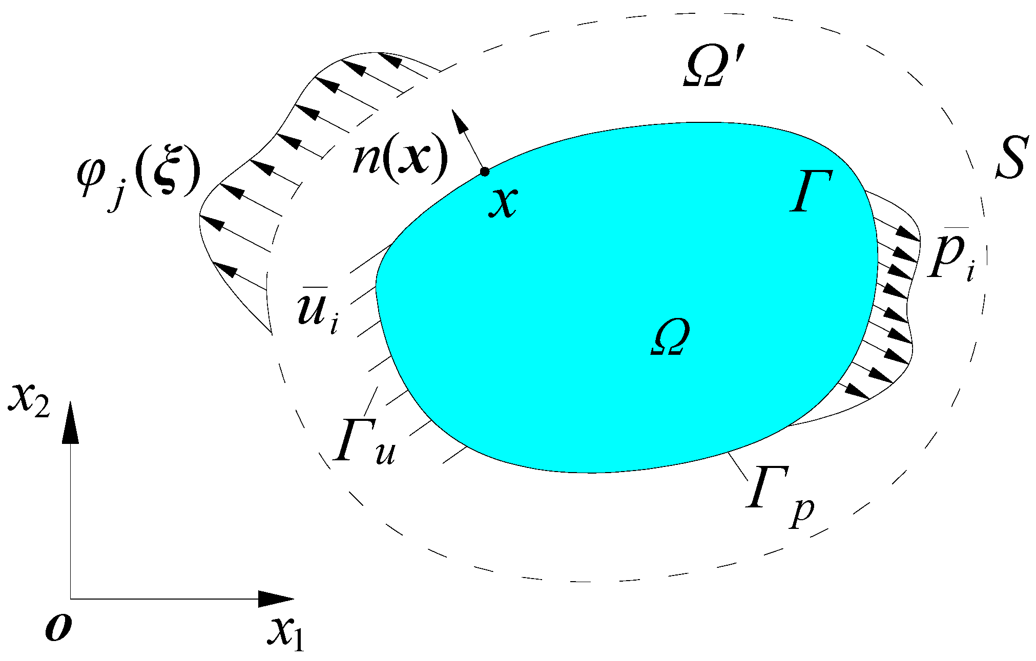
3. The Virtual Boundary Meshless Galerkin Method with the Partial Differential Equation on the Weak Term

The following is an overview of VBEM. Suppose that Ω indicates the computational domain, whose boundaries are recorded as Γ in Figure 1. The external normal of the point x on Γ is n(x). Expanding Ω along n(x), a virtual domain Ω’ can be obtained, whose boundaries are defined as S. Assume the continuous virtual load ${\phi }_j(\xi )$($j=1,2$) at any point $\xi$ on S. The ith direction displacement and surface force of the point $x$ are $u_i(x)$ and $p_i(x)$, respectively. The following equations are used.

$$u_i(x)={\displaystyle {\int }_S{u}_{ij}^{*}}(x,\xi ){\phi }_j(\xi )dS$$

(12)

$$p_i(x)={\displaystyle {\int }_S{p}_{ij}^{*}}(x,\xi ){\phi }_j(\xi )dS$$

(13)

where $u_{ij}^{*}$ and $p_{ij}^{*}$ are the Kevin fundamental solutions of displacement and surface force of 2D elastic problem.

The boundary conditions of Equations (12) and (13) are

$$u_i(x)={\overline{u}}_i(x)\hspace{1em}\hspace{1em}(x\in {\Gamma }_u)$$

(14)

$$p_i(x)={\overline{p}}_i(x)\hspace{1em}\hspace{1em}(x\in {\Gamma }_p)$$

(15)

where, ${\overline{u}}_i(x)$ is the known displacement on the real boundary ${\Gamma }_u$ with known displacement. ${\overline{p}}_i(x)$ is the known surface force on the real boundary ${\Gamma }_p$ with known surface force. ${\Gamma }_u\cup {\Gamma }_p=\Gamma$ and ${\Gamma }_u\cap {\Gamma }_p=Ø$ (null set).

The partial differential equation on the weak term can be established with Equations (14) and (15), using the Galerkin method of weighted residual method, namely,

$$w_1\underset{x\in {\Gamma }_u}{{\displaystyle \int }}\left[u_i(x)-{\overline{u}}_i(x)\right]d\Gamma (x)+w_2\underset{x\in {\Gamma }_p}{{\displaystyle \int }}\left[p_i(x)-{\overline{p}}_i(x)\right]d\Gamma (x)=0$$

(16)

where $w_1$ and $w_2$ are the weighted coefficients obtained using the Galerkin method, respectively, $w_1=\delta u_i(x)$, $w_2=\delta p_i(x)$.

The continuous virtual load ${\phi }_j(\xi )$ can be construed by Equation (10) using RBFCS, namely,

$${\phi }_j(\xi )\approx {\displaystyle \sum _{l=1}^{m}N(\xi ,{\xi }_l)\cdot {\phi }_j({\xi }_l)}$$

(17)

where m is the virtual node number within the local compact support domain of $\xi$; ${\phi }_j({\xi }_l)$ is the virtual load in the j direction of the lth virtual node ${\xi }_l$; and $N(\xi ,{\xi }_l)$ is the shape function of ${\xi }_l$ about calculation point $\xi$.

Equations (12) and (13) can be rewritten as, respectively,

$$\begin{array}{ll}{u}_i(x)& \approx {\displaystyle {\int }_S{u}_{ij}^{*}(x,\xi ){\phi }_j(\xi )dS}\\ & ={\displaystyle \sum _{e^{\prime }=1}^{m_{e^{\prime }}}{\displaystyle \sum _{g^{\prime }=1}^{e_{e^{\prime }}}w({\xi }_{e^{\prime }}^{g^{\prime }})J^{\prime }{u}_{ij}^{*}(x,{\xi }_{e^{\prime }}^{g^{\prime }}){\phi }_j({\xi }_{e^{\prime }}^{g^{\prime }})}}\\ & ={\displaystyle \sum _{e^{\prime }=1}^{m_{e^{\prime }}}{\displaystyle \sum _{g^{\prime }=1}^{e_{e^{\prime }}}w({\xi }_{e^{\prime }}^{g^{\prime }})J^{\prime }{u}_{ij}^{*}(x,{\xi }_{e^{\prime }}^{g^{\prime }}){\displaystyle \sum _{l=1}^{m}N({\xi }_{e^{\prime }}^{g^{\prime }},{\xi }_l)\cdot {\phi }_j({\xi }_l)}}}\\ & =U\cdot \phi \end{array}$$

(18)

$$\begin{array}{ll}{p}_i(x)& \approx {\displaystyle {\int }_S{p}_{ij}^{*}(x,\xi ){\phi }_j(\xi )dS}\\ & ={\displaystyle \sum _{e^{\prime }=1}^{m_{e^{\prime }}}{\displaystyle \sum _{g^{\prime }=1}^{e_{e^{\prime }}}w({\xi }_{e^{\prime }}^{g^{\prime }})J^{\prime }{p}_{ij}^{*}(x,{\xi }_{e^{\prime }}^{g^{\prime }}){\phi }_j({\xi }_{e^{\prime }}^{g^{\prime }})}}\\ & ={\displaystyle \sum _{e^{\prime }=1}^{m_{e^{\prime }}}{\displaystyle \sum _{g^{\prime }=1}^{e_{e^{\prime }}}w({\xi }_{e^{\prime }}^{g^{\prime }})J^{\prime }{p}_{ij}^{*}(x,{\xi }_{e^{\prime }}^{g^{\prime }}){\displaystyle \sum _{l=1}^{m}N({\xi }_{e^{\prime }}^{g^{\prime }},{\xi }_l)\cdot {\phi }_j({\xi }_l)}}}\\ & =P\cdot \phi \end{array}$$

(19)

where $m_{e^{\prime }}$ is the virtual element number of S; $e_{e^{\prime }}$ is the Gauss point number of every virtual element; $w({\xi }_{e^{\prime }}^{g^{\prime }})$ is the Gauss numerical integral coefficient of virtual element; and $J^{\prime }$ is the Jacobian of virtual element. Note that numerical integration of Equations (18) and (19) need to use the background grid. Assume that NV is the whole virtual node number, then the unknown matrix $\phi$, the known coefficient matrices $U$ and $P$ are as follows:

$$\begin{array}{ll}\phi & ={\left[{\phi }_1({\xi }_1)\hspace{1em}{\phi }_2({\xi }_1)\hspace{1em}\cdots \hspace{1em}{\phi }_j({\xi }_l)\hspace{1em}\cdots \hspace{1em}{\phi }_1({\xi }_{NV})\hspace{1em}{\phi }_2({\xi }_{NV})\right]}^{\mathrm{T}}\\ & ={\left[{\phi }_1\hspace{1em}{\phi }_2\hspace{1em}\cdots \hspace{1em}{\phi }_s\hspace{1em}\cdots \hspace{1em}{\phi }_{2NV}\right]}^{\mathrm{T}}\end{array}$$

(20)

$$\begin{array}{ll}U& =\left[U_1({\xi }_1)\hspace{1em}{U}_2({\xi }_1)\hspace{1em}\cdots \hspace{1em}{U}_j({\xi }_l)\hspace{1em}\cdots \hspace{1em}{U}_1({\xi }_{NV})\hspace{1em}{U}_2({\xi }_{NV})\right]\\ & =\left[U_1\hspace{1em}{U}_2\hspace{1em}\cdots \hspace{1em}{U}_s\hspace{1em}\cdots \hspace{1em}{U}_{2NV}\right]\end{array}$$

(21)

$$\begin{array}{ll}P& =\left[P_1({\xi }_1)\hspace{1em}{P}_2({\xi }_1)\hspace{1em}\cdots \hspace{1em}{P}_j({\xi }_l)\hspace{1em}\cdots \hspace{1em}{P}_1({\xi }_{NV})\hspace{1em}{P}_2({\xi }_{NV})\right]\\ & =\left[P_1\hspace{1em}{P}_2\hspace{1em}\cdots \hspace{1em}{P}_s\hspace{1em}\cdots \hspace{1em}{P}_{2NV}\right]\end{array}$$

(22)

Note that C is the Gauss point number within the local compact support domain of the lth virtual node on the boundary S, then meanings $U_j({\xi }_l)$ and $P_j({\xi }_l)$ are the summation of integral terms of displacement and surface force for the virtual loads in the jth direction of ${\xi }_l$.

$$U_j({\xi }_l)={\displaystyle \sum _{c=1}^{C}w({\xi }_c^{g^{\prime }})J^{\prime }{u}_{ij}^{*}(x,{\xi }_c^{g^{\prime }})N({\xi }_c^{g^{\prime }},{\xi }_l)}$$

(23)

$$P_j({\xi }_l)={\displaystyle \sum _{c=1}^{C}w({\xi }_c^{g^{\prime }})J^{\prime }{p}_{ij}^{*}(x,{\xi }_c^{g^{\prime }})N({\xi }_c^{g^{\prime }},{\xi }_l)}$$

(24)

Equation (16) can be expressed as

$$w_1\sum _{e=1}^{m_u}\sum _{g=1}^{e_u}\left[u_i(x)-{\overline{u}}_i(x)\right]\overline{w}({\xi }_e^g)J+w_2\sum _{e=1}^{m_p}\sum _{g=1}^{e_p}\left[p_i(x)-{\overline{p}}_i(x)\right]\overline{w}({\xi }_e^g)J=0$$

(25)

where $m_u$ and $m_p$ are the number of real elements on ${\Gamma }_u$ and ${\Gamma }_p$, respectively; $e_u$ and $e_p$ the Gauss point number within real elements on ${\Gamma }_u$ and ${\Gamma }_p$, respectively; $\overline{w}({\xi }_e^g)$ is the Gauss numerical integral coefficient of real element; and $J$ is the Jacobian of real element.

Considering that $\partial u_i(x)/\partial {\phi }_s=U_s$ and $\partial p_i(x)/\partial {\phi }_s=P_s$, Equation (25) is rewritten as a matrix

$$A\phi =B$$

(26)

where $A={[A_{st}]}_{2NV\times 2NV}$ is a symmetric coefficient matrix; $\phi$ is the unknown matrix of the entire virtual loads; and $B={[b_s]}_{2NV\times 1}$ is the known matrix about the boundary conditions. $A_{st}$ and $b_s$ are

$$A_{st}={\displaystyle \sum }_{e=1}^{m_u}{\displaystyle \sum }_{g=1}^{e_u}\overline{w}({\xi }_e^g)J{U}_s{U}_t+{\displaystyle \sum }_{e=1}^{m_p}{\displaystyle \sum }_{g=1}^{e_p}\overline{w}({\xi }_e^g)J{P}_s{P}_t$$

(27)

$$b_s={\displaystyle \sum }_{e=1}^{m_u}{\displaystyle \sum }_{g=1}^{e_u}\overline{w}({\xi }_e^g)J{U}_s{\overline{u}}_i(x)+{\displaystyle \sum }_{e=1}^{m_p}{\displaystyle \sum }_{g=1}^{e_p}\overline{w}({\xi }_e^g)J{P}_s{\overline{p}}_i(x)$$

(28)

Therefore, $w_1=U_s$ and $w_2=P_s$ in Equation (16).

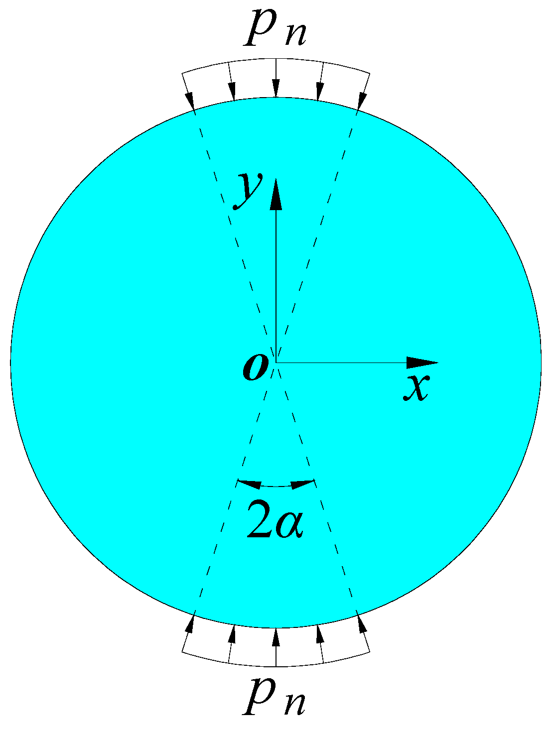
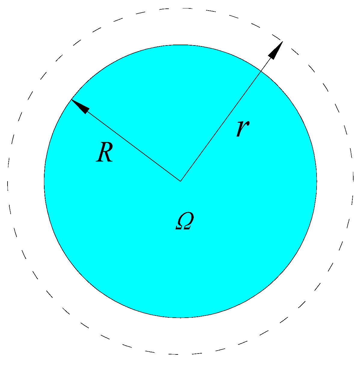
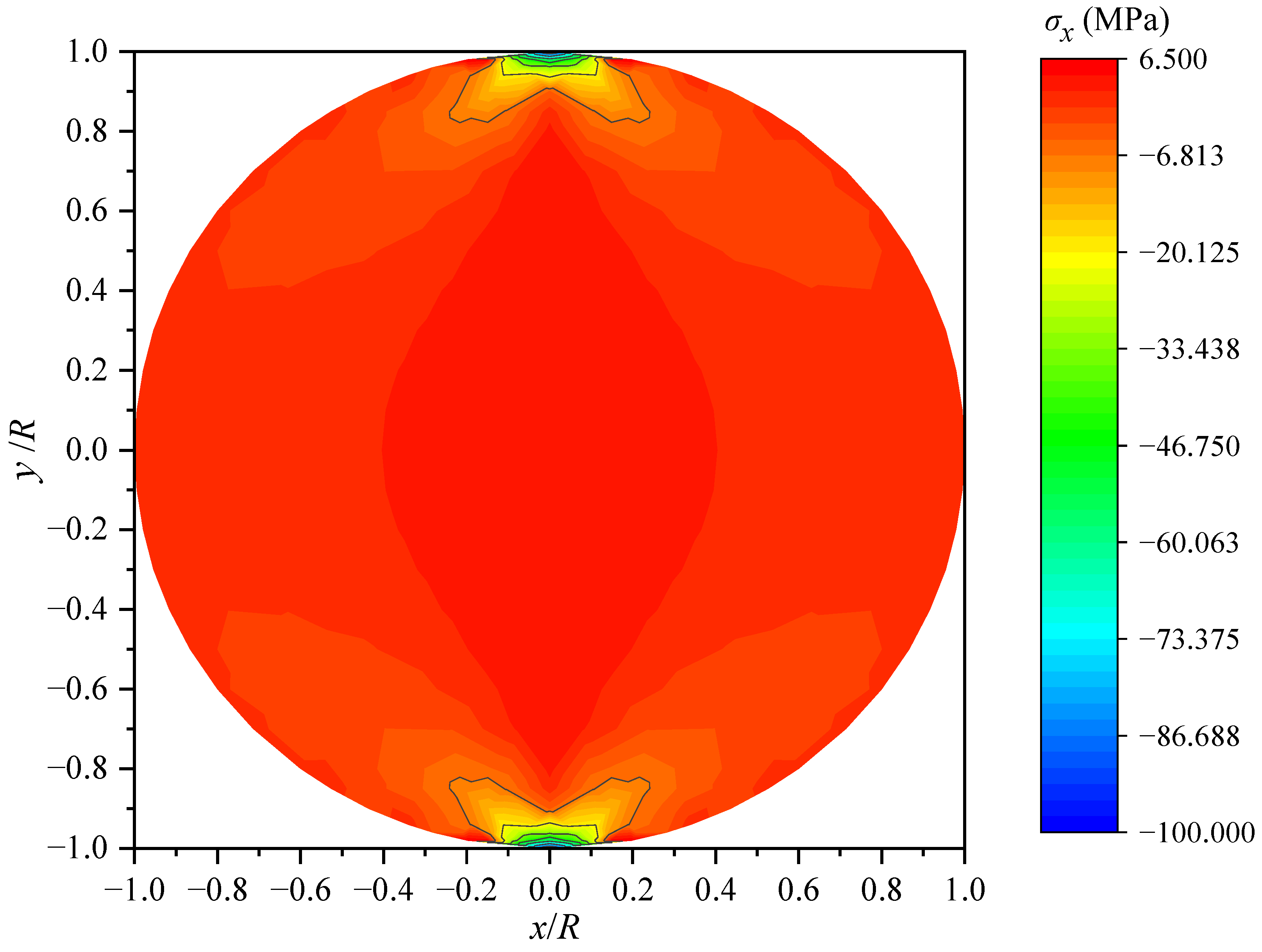
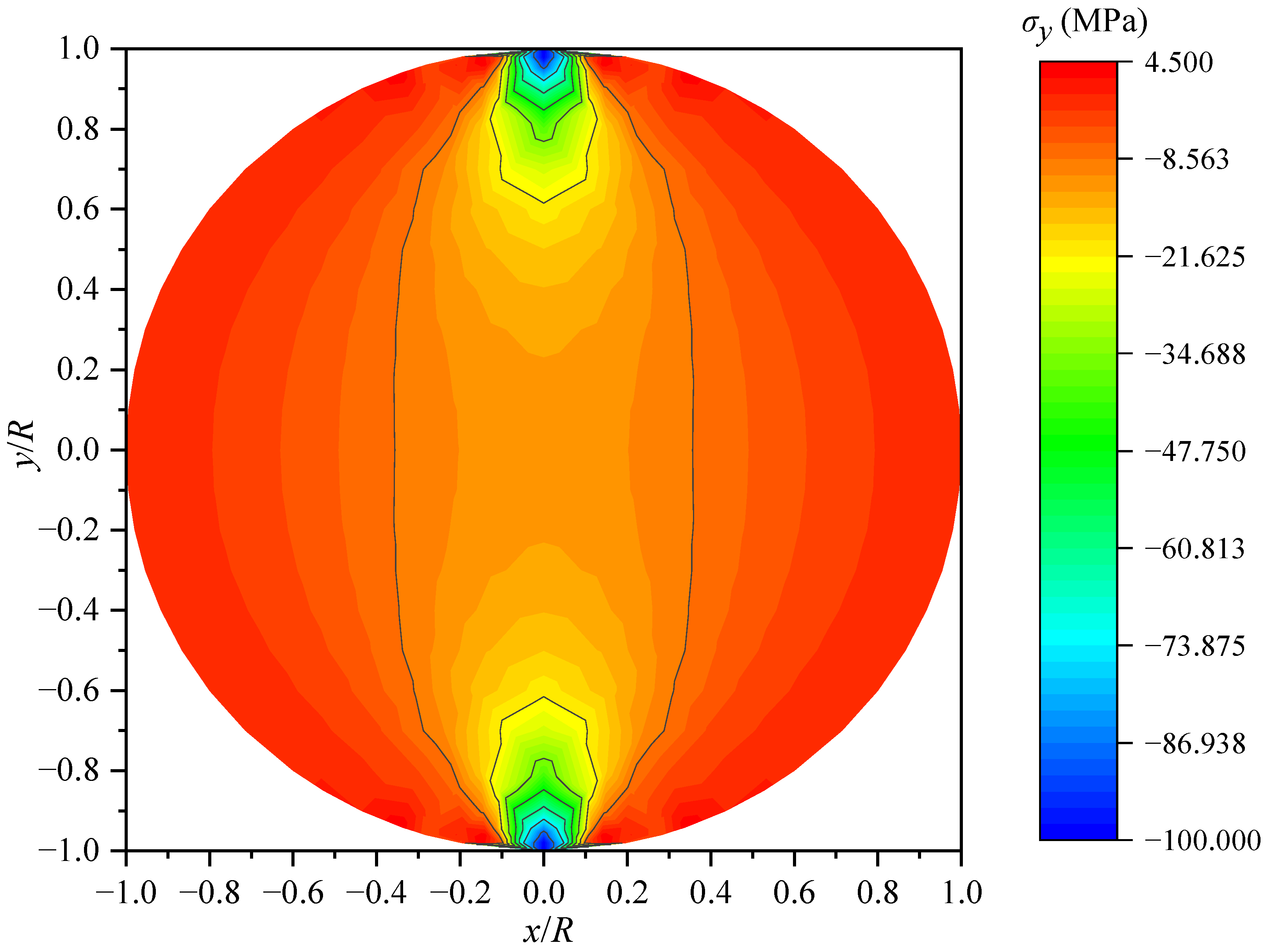
4. Numerical Example: The Axial Compression on the Part Boundary of the Circular Shaft

The part boundary of the circular shaft is subjected to the axial compression. The computational model is shown in Figure 2. The radius R of the circular shaft is 1 dm, 2α = 7.2°, p_n = 100 MPa, elastic modulus E = 2200 MPa, and Poisson ratio v = 0.1. The numerical example is viewed as 2D stress problem.

The discretization of the circular shaft in Figure 3: 200 real elements are evenly distributed on the real boundary Γ; the number of virtual boundary elements, namely, 100, is taken as the general number of real boundary elements, and the circular virtual boundary S (r = 1.4) is evenly divided. The number of virtual elements and the number of virtual nodes are identical. Virtual nodes are positioned at the midpoint of their virtual elements. The construction of the virtual source function utilizes eight virtual nodes. Each virtual or real element adopts four Gauss points for integration by using RBFCS.

Here, the stresses σ_x and σ_y at points (0, y) and (x, 0) are calculated, respectively.

Some scholars also calculate the numerical example. Jaeger J.C. and Hoskins E.R. [16] employ the complex function method to obtain the analytical solution (Ass).

The analytical solutions of stresses along the y-axis (ρ = y/R):

$$\begin{array}{c}{\sigma }_x=\frac{-2p_n}{\pi }\left[\frac{\left(1-{\rho }^2\right)\sin 2\alpha }{\left(1-2{\rho }^2\cos 2\alpha +{\rho }^4\right)}-\arctan \left(\frac{1+{\rho }^2}{1-{\rho }^2}\tan \alpha \right)\right]\\ {\sigma }_y=\frac{2p_n}{\pi }\left[\frac{\left(1-{\rho }^2\right)\sin 2\alpha }{\left(1-2{\rho }^2\cos 2\alpha +{\rho }_{}^4\right)}+\arctan \left(\frac{1+{\rho }^2}{1-{\rho }^2}\tan \alpha \right)\right]\\ {\tau }_{xy}=0\end{array}$$

The analytical solutions of stresses along the x-axis (ρ = x/R):

$$\begin{array}{c}{\sigma }_x=\frac{-2p_n}{\pi }\left[\frac{\left(1-{\rho }^2\right)\sin 2\alpha }{\left(1+2{\rho }^2\cos 2\alpha +{\rho }^4\right)}-\arctan \left(\frac{1-{\rho }^2}{1+{\rho }^2}\tan \alpha \right)\right]\\ {\sigma }_y=\frac{2p_n}{\pi }\left[\frac{\left(1-{\rho }^2\right)\sin 2\alpha }{\left(1+2{\rho }^2\cos 2\alpha +{\rho }_{}^4\right)}+\arctan \left(\frac{1-{\rho }^2}{1+{\rho }^2}\tan \alpha \right)\right]\\ {\tau }_{xy}=0\end{array}$$

Kuang G.N., Xiong Z.N., and Song Z.X. [17] apply the boundary element method (BEM), virtual stress method (VSM), and displacement discontinuity method (DDM) to achieve the results. Kuang G.N. et al. take the quarter of the circular shaft as the computational model, taking into account the symmetry of this problem; namely, the quarter of circular boundary and two radial boundaries are equally partitioned into 50, 20, and 20 elements, and 200 elements on the whole circular boundary; however, the virtual element number is 100 in this paper, on account of the virtual load as the unknown physical quantity. The stresses σ_x (MPa) and σ_y (MPa) at points (0, y) and (x, 0) are shown in

Table 1. The stresses σ_x (MPa) and σ_y (MPa) at points (x = 0 and y dm) of the axial compression on the part boundary of the circular shaft.

Coordinates		(0, 0)	(0, 0.1)	(0, 0.2)	(0, 0.3)	(0, 0.4)	(0, 0.5)	(0, 0.6)	(0, 0.7)	(0, 0.8)
σx	BEM	3.936	3.934	3.928	3.917	3.895	3.853	3.761	3.519	2.644
	VSM	3.914	3.913	3.909	3.901	3.885	3.851	3.774	3.562	2.766
	DDM	3.955	3.955	3.954	3.951	3.944	3.926	3.876	3.714	3.009
	the paper	3.979	3.978	3.973	3.965	3.948	3.913	3.836	3.621	2.791
	Ass	3.979	3.978	3.973	3.965	3.948	3.913	3.836	3.621	2.792
σy	BEM	−11.925	−12.082	−12.574	−13.462	−14.875	−17.061	−20.514	−26.333	−27.410
	VSM	−11.871	−12.026	−12.513	−13.392	−14.791	−16.954	−20.370	−26.122	−37.065
	DDM	−12.003	−12.162	−12.659	−13.558	−14.991	−17.214	−20.744	−26.740	−38.322
	the paper	−11.979	−12.139	−12.638	−13.542	−14.982	−17.216	−20.758	−26.766	−38.330
	Ass	−11.979	−12.139	−12.638	−13.542	−14.982	−17.216	−20.758	−26.766	−38.332

and

Table 2. The stresses σ_x (MPa) and σ_y (MPa) at points (x dm and y = 0) of the axial compression on the part boundary of the circular shaft.

Coordinates		(0, 0)	(0.1, 0)	(0.2, 0)	(0.3, 0)	(0.4, 0)	(0.5, 0)	(0.6, 0)	(0.7, 0)	(0.8, 0)
σx	BEM	3.936	3.783	3.359	2.752	2.074	1.426	0.877	0.462	0.186
	VSM	3.914	3.763	3.343	2.741	2.069	1.425	0.879	0.464	0.187
	DDM	3.955	3.800	3.372	2.760	2.077	1.424	0.872	0.454	0.176
	the paper	3.979	3.824	3.393	2.778	2.092	1.438	0.885	0.469	0.193
	Ass	3.979	3.824	3.393	2.778	2.092	1.438	0.885	0.469	0.193
σy	BEM	−11.925	−11.616	−10.742	−9.437	−7.886	−6.255	−4.680	−3.245	−1.992
	VSM	−11.871	−11.565	−10.700	−9.412	−7.875	−6.261	−4.701	−3.279	−2.036
	DDM	−12.003	−11.692	−10.814	−9.505	−7.949	−6.316	−4.741	−3.309	−2.060
	the paper	−11.979	−11.666	−10.779	−9.459	−7.889	−6.242	−4.654	−3.210	−1.951
	Ass	−11.979	−11.686	−10.779	−9.459	−7.889	−6.242	−4.654	−3.210	−1.951

, respectively. x and y are dm. The computational results show that the problem can be solved by the method in this paper and the computational accuracy is proved. The stress contour maps of σ_x, σ_y, and τ_xy are shown in Figure 4, Figure 5 and Figure 6 using the VBMGM according to the paper. The vertical and horizontal coordinates are dimensionless, as shown in Figure 4, Figure 5 and Figure 6.

5. Conclusions

The VBMGM is established and this method is achieved by using the Galerkin method and RBFCS to approximate the virtual load on the virtual boundary; therefore, the proposed method offers the benefits of BEM, the meshfree method, and the Galerkin method.

The numerical meanings of the weighted coefficients, namely, the partial derivative displacement or surface force, are clear, and the detailed numerical discrete formula of the VBMGM is derived.

The stresses σ_x and σ_y at points (0, y) and (x, 0) of the axial compression on the part boundary of the circular shaft are calculated, and the results are compared with the boundary element method, the virtual stress method, the displacement discontinuity method, and the analytical solution. The results show that the proposed method is accurate.

Because it is easy to program, the VBMGM should be expanded to deal with other boundary value problems, such as the steel connection, the multi-hole shear wall, the corbel structure of hydropower station, and so on.

References

1. Padilla, A.; Genedy, M.; Knight, E.E.; Rougier, E.; Stormont, J.; Taha, M.M.R. Monitoring Postpeak Crack Propagation in Concrete in the Brazilian Tension Test. J. Mater. Civ. Eng. 2022, 34, 04022110-1–04022110-10. [Google Scholar] [CrossRef]
2. Efimov, V.P. Brazilian Tensile Strength Testing. J. Min. Sci. 2021, 57, 922–932. [Google Scholar] [CrossRef]
3. Zhang, J.; Li, X.X.; Li, Y.W.; Tao, F.Y.; Yan, M.S. Experimental research and numerical simulation: Strength and rupture patterns of coal under Brazilian tensile test. Int. J. Oil Gas Coal Technol. 2021, 26, 225–244. [Google Scholar] [CrossRef]
4. Torabi, A.R.; Motamedi, M.A.; Bahrami, B.; Noushak, M.; Cicero, S.; Alvarez, J.A. Determination of Translaminar Notch Fracture Toughness for Laminated Composites Using Brazilian Disk Test. Polymers 2022, 14, 3246. [Google Scholar] [CrossRef] [PubMed]
5. Xiao, P.; Zhao, G.Y.; Liu, H.X. Failure Transition and Validity of Brazilian Disc Test under Different Loading Configurations: A Numerical Study. Mathematics 2022, 10, 2681. [Google Scholar] [CrossRef]
6. Haeri, H.; Shahriar, K.; Marji, M.F.; Moarefvand, P. Experimental and numerical study of crack propagation and coalescence in pre-cracked rock-like disks. Int. J. Rock Mech. Min. Sci. 2014, 67, 20–28. [Google Scholar] [CrossRef]
7. Lanaro, F.; Sato, T.; Stephansson, O. Microcrack modelling of Brazilian tensile tests with the boundary element method. Int. J. Rock Mech. Min. Sci. 2009, 46, 450–461. [Google Scholar] [CrossRef]
8. Cheng, A.H.D.; Cheng, D.T. Heritage and early history of the boundary element method. Eng. Anal. Bound. Elem. 2005, 29, 268–302. [Google Scholar] [CrossRef]
9. Sun, H.C.; Li, X.H.; Zhang, L. Virtual Boundary Element-Collocation Method for Solving Problems of Elasticity. Comput. Struct. Mech. Appl. 1991, 8, 15–23. (In Chinese) [Google Scholar]
10. Sun, H.C.; Zhang, L.Z.; Xu, Q.; Zhang, Y.M. Nonsingularity Boundary Element Methods; Dalian University of Technology Press: Dalian, China, 1999. (In Chinese) [Google Scholar]
11. Xu, Q.; Sun, H.C. Virtual boundary element least-square collocation method. Chin. J. Comput. Mech. 1997, 14, 166–173. (In Chinese) [Google Scholar]
12. Xu, Q.; Zhang, Z.J.; Si, W. Virtual boundary meshless least square collocation method for calculation of 2D multi-domain elastic problems. Eng. Anal. Bound. Elem. 2012, 36, 696–708. [Google Scholar] [CrossRef]
13. Yang, D.S.; Xu, Q. Virtual boundary meshless least square integral method with moving least squares approximation for 2D elastic problem. Eng. Anal. Bound. Elem. 2013, 37, 616–623. [Google Scholar] [CrossRef]
14. Xu, Q.; Yang, D.S. Solving multi-domain 2D heat conduction problems by the least squares collocation method with RBF interpolation on virtual boundary. Eng. Anal. Bound. Elem. 2014, 42, 37–44. [Google Scholar] [CrossRef]
15. Liu, G.R.; Gu, Y.T. Boundary meshfree methods based on the boundary point interpolation methods. Eng. Anal. Bound. Elem. 2004, 28, 475–487. [Google Scholar] [CrossRef]
16. Jaeger, J.C.; Hoskins, E.R. Rock failure under the confined brazilian test. J. Geophys. Res. 1966, 71, 2651–2659. [Google Scholar] [CrossRef]
17. Kuang, G.N.; Xiong, Z.N.; Song, Z.X. Boundary Element Method in Practical Engineering; Chinese Railway Press: Beijing, China, 1989. (In Chinese) [Google Scholar]
Figure 1. Diagrammatic sketch of the virtual boundary method.
Applsci 12 11806 g001
Figure 2. The axial compression on the part boundary of the circular shaft.
Applsci 12 11806 g002
Figure 3. Discretization of the axial compression on the part boundary of the circular shaft.
Applsci 12 11806 g003
Figure 4. σx contour map of the axial compression on the part boundary of the circular shaft.
Applsci 12 11806 g004
Figure 5. σy contour map of the axial compression on the part boundary of the circular shaft.
Applsci 12 11806 g005
Figure 6. τxy contour map of the axial compression on the part boundary of the circular shaft.
Applsci 12 11806 g006